Conceptually Simple Method for Optimizing Model Computations in MATLAB Simulink

Abstract

This article describes a procedure for enhancing computational accuracy in MATLAB’s Simulink and Simscape environments, as illustrated through specific example cases. It builds on earlier published by the authors’ team, which demonstrated the practical application of the Simscape Multibody tool—originally designed for dynamic and kinematic analyses—for making static computations in truss systems. Simscape Multibody serves as an effective platform for realistic and simplified simulations of mechanical components, incorporating various mechanical properties. Consequently, it is valuable in simulating mechatronic systems, where the integration of mechanics, electronics, control systems, and information technologies is essential. Multiple models were tested and analyzed across different scenarios to facilitate a comparative assessment of the results. The significance of this work lies in its achievement of highly accurate computational results without relying purely on theoretical calculations, with superior values in terms of accuracy. The primary objective was to provide a clear and practical description of a simple procedure for improving computational accuracy, based on scaling.

1. Introduction

This article builds upon our previous publication [1], which addressed the analysis of a truss system using MATLAB–Simscape Multibody [2,3] version 24.1.0.2628055 (R2024a) Update 4. It presents additional examples to further clarify and elaborate on this computational approach. The paper also provides a more detailed explanation of how an additional scaling [4] procedure can be utilized to enhance computational accuracy within the Simulink environment. To ensure the reliability of the simulation results, the system was also analyzed within the framework of Hooke’s law (linear elastic behavior). Due to the inherent complexity of such computations, particularly when dealing with more sophisticated structural systems, a range of software tools are typically employed. When the primary objective is to determine deformations and internal forces in components that may be part of a broader mechatronic system [5,6], Simscape Multibody proves to be a useful toolbox. It serves as a successor to the formerly used SimMechanics [7], which has been widely applied in mechanical simulations, as demonstrated in [8,9]. The approach described herein enables a notable increase in computational accuracy without significantly extending the simulation time. Using this approach, computational accuracy can be improved to the level of approximately 10⁻⁶. Our testing has also demonstrated that this approach can, to a certain extent, be applied more broadly across the Simulink platform. Most toolboxes already have scaling by Nominal Values [10] implemented.

While the Multibody toolbox does not constitute a fully fledged finite element analysis (FEA) tool—particularly with regard to large deformations, nonlinear material strength behavior, and overall computational capacity—it nonetheless offers considerable value to users operating within the Simulink environment, especially when integrating additional toolboxes. It allows users to avoid constructing excessively complex mechanical models. The Multibody library includes a set of components known as flexible bodies [3], which represent elements capable of elastic deformation under combined loading conditions, specifically tension, compression, bending, and torsion [11]. The stiffness and inertia of these bodies derive from their geometric and material properties. The computational principle applied to bars follows the Euler–Bernoulli beam theory [12] (pp. 174–220), which is suitable for modeling truss systems. The computational setup also includes the visualization of results based on user-defined input parameters. For comparative purposes, each example is accompanied by results obtained through analytical procedures. In this context, the term “bars” refers to structural members with uniform cross-sections, fixed at both ends via joints. The connection point of at least two such bars is defined as a node. It should also be noted that under compressive loading, buckling may occur [13] (pp. 483–507), resulting in a loss of stability and deflection of the bar through buckling from its original axis. This article does not address the assessment of buckling stability [14] in compression-loaded bars. For detailed analyses and theoretical background related to the stability of structures, the reader is referred to [15] (pp. 449–511).

Ultimately, the article deals in more detail with the explanation of a simple procedure for improving computational accuracy, using simplified scaling depending on a single input variable. Scaling by nominal values allows you to set the value of a variable for the solver in such a range that the dynamics of the calculation of all variables in a given system are matched. This increases the robustness of the simulation. The benefit is faster convergence of the solution and maintaining a minimum iteration step size. In Simscape Multibody™, there is no scaling system [10] in the sense that we know it for most Simscape toolboxes using nominal values. This can be solved by changing the proportion of the variable, but this may result in a change in the output values. If we do not want to change the number of parameters and adapt the model for numerical purposes, we only shifted the value of the input quantity. Due to this simple adjustment, it is of course not possible to maintain the calculation accuracy in the same class (10⁻⁶) with a dynamically changing input variable (in our case F_{load m}). But it is especially suitable for steady states. In our case, for example, for static calculations. The most effective is to use automatic solver selection. The software will use an algorithm to select the solver (method) and the maximum step size. We emphasize that this is not a description of a new method, but a better use of the potential of existing tools. For the input of the scaling procedure, we can simply write input{F_{load m}/con} and for the outputs{(F, N, δ) × con}. This procedure, which is used in the examples, can bring a benefit in terms of accuracy of about two orders of magnitude.

2. Illustrative Planar Examples

This section presents selected examples of truss systems, which are used to demonstrate methods for achieving maximum computational accuracy in Simscape Multibody. In each example, the models differ slightly in the type of bar employed and in the way in which the node is implemented. These variations are deliberate, as we will later examine how the toolbox handles the visualization of structural loading. The models are partially inspired by publicly available sources [16], which have been adapted for various configurations.

The first tested structure is the truss system shown in Figure 1. It consists of five nodes and seven bars, and is once externally statically indeterminate (see, e.g., [17], pp. 107–108).

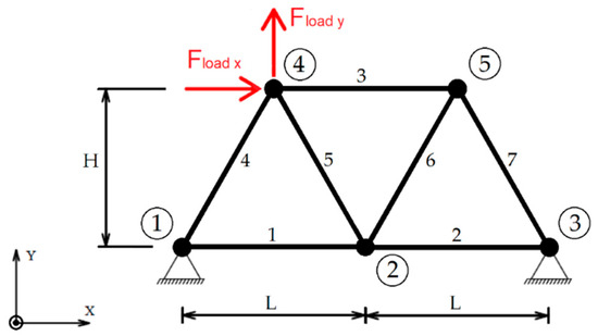
Figure 1. Example 1. A schematic of the truss system subjected to the force vector F_load at Node_4.

2.1. Example 1: Three Modeling Variants

A schematic of the truss system used in Example 1 is shown in Figure 1. The structure was experimentally modeled using three different approaches (models):

• Model 1.1 is composed of Euler–Bernoulli beams and joints.
• Model 1.2 serves as an experimental variant. It also employs Euler–Bernoulli beams, but it uses solid joints. This configuration does not conform to the assumptions of the theoretical model, as the nodes do not incorporate movable joints.
• Model 1.3 consists of rigid bars with one degree of freedom (1 DOF) and joints. This model most closely resembles the conventional standards used in static structural analysis software.

The truss system is subjected to a force vector applied at Node_4. All bars have identical cross-sections.

2.1.1. Model 1.1: Truss System Composed of Euler–Bernoulli Beams and Joints

Model 1.1, constructed in Simscape Multibody, is depicted in Figure 2. The same block structure is used for Model 1.2 and Model 1.3. All functional models are available at [18].

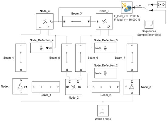
Figure 2. Models 1.1, 1.2, and 1.3. The truss system subjected to the force vector F_load at Node_4, modeled in MATLAB–Simscape Multibody as defined in Figure 1.

Figure 3 illustrates the subsystem of a truss bar, based on the Bernoulli beam model. Only axial force is considered. All truss bars in simulation Model 1.1 and Model 1.2 are identical in structure and constructed as follows:

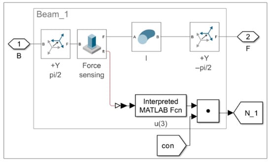
Figure 3. Models 1.1 and 1.2. An example of a truss bar subsystem, labeled Beam_1.

Blocks of the “Rigid Transform” type are used to rotate the truss bar into the desired plane about the y–axis of the World Frame. The value of the force vector N₁ is obtained directly from the “Weld Joint” block using Total force sensing. The “Interpreted MATLAB Function” block—specifically, its output u(3)—extracts the z-component of the force vector N₁ acting within the bar. Although the manufacturer recommends using “User-Defined Functions” [19] (p. 344) or their online counterparts [20], in order to improve computational speed, we have chosen the “Interpreted MATLAB Function” block, due to its greater flexibility in parameter syntax. The block that physically represents the truss bar, labeled Beam, is of the type “Flexible Cylindrical Beam”. Within this block, key physical parameters are specified: the bar length l, the diameter d, the Young’s modulus of elasticity E, the shear modulus G, the material density (Density), and the coefficients of proportional Rayleigh damping [21], denoted as b_m and b_k.

Figure 4 illustrates the subsystems by node in Model 1.1 and Model 1.3. While structurally similar, each node exhibits differences in configuration and in the specification of the initial position state (in radians). All nodes are constructed using joints.

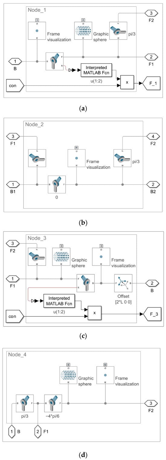
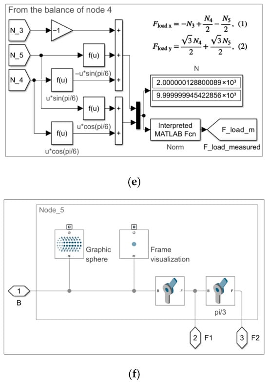
Figure 4. Model 1.1 and Model 1.3. Subsystems by node: (a) Node_1; (b) Node_2; (c) Node_3; (d) Node_4; (e) measurement of the F_{load m} force at Node_4; (f) Node_5.

The F_{load m} force essentially serves as a means of verifying the computed F_load force. It is derived from the internal forces within the system, specifically based on the equilibrium conditions at Node_4.

$$\sum F_x=0; F_{\mathrm{l}\mathrm{o}\mathrm{a}\mathrm{d} x}+N_3-{\displaystyle \frac{N_4}{2}}+{\displaystyle \frac{N_5}{2}}=0$$

(1)

$$\sum F_y=0; F_{\mathrm{l}\mathrm{o}\mathrm{a}\mathrm{d} y}-{\displaystyle \frac{\sqrt{3}{·N}_4}{2}}-{\displaystyle \frac{\sqrt{3}{·N}_5}{2}}=0$$

(2)

The F_load force represents the external load applied to the system. In cases where multiple external forces act on the system, the one with the highest magnitude is selected for validation purposes.

2.1.2. Model 1.2: Truss System Composed of Euler–Bernoulli Beams and Solid Joints

The truss system defined as Model 1.2, constructed in Simscape Multibody, features the same block configuration as shown in Figure 2. The only distinction lies in the implementation of the nodes.

Figure 5 illustrates the subsystems by node in Model 1.2. Each node differs in its configuration and initial position state (in radians). The nodes are composed of solid joints.

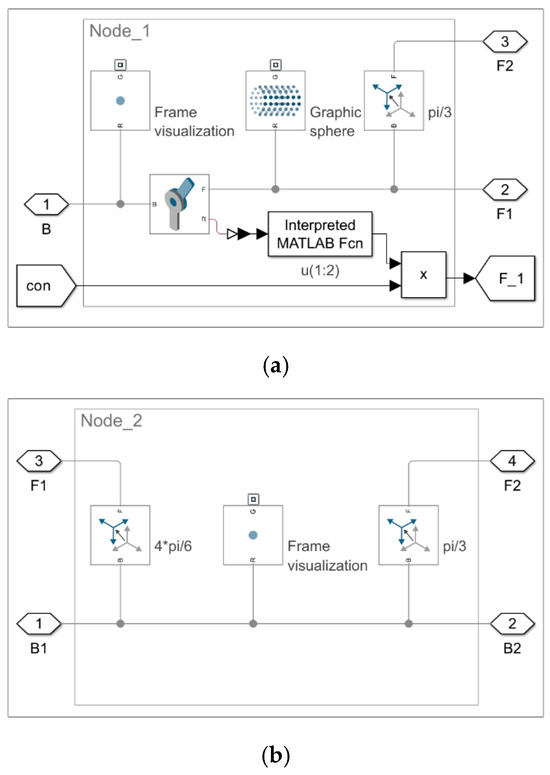
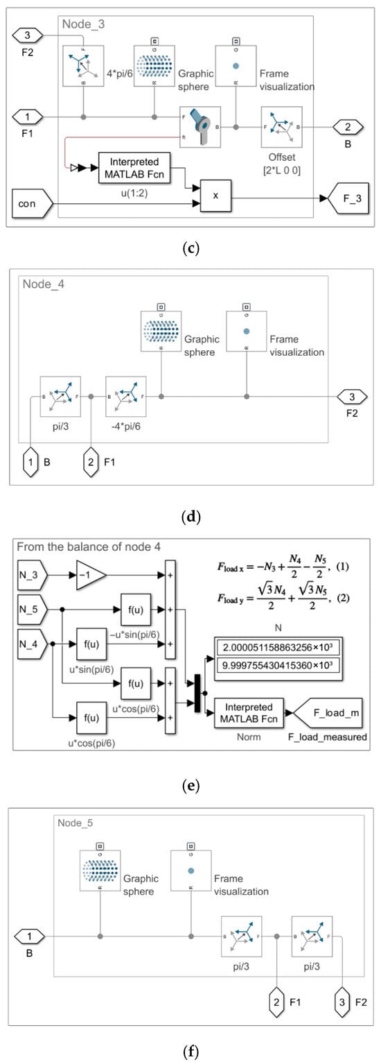
Figure 5. Model 1.2. Subsystems by node: (a) Node_1; (b) Node_2; (c) Node_3; (d) Node_4; (e) measurement of the F_{load m} force at Node_4; (f) Node_5.

As in the previous case, the F_{load m} force is derived from the equilibrium conditions at Node_4, as expressed in Equations (1) and (2). However, this interpretation is not entirely accurate in this context, since the nodes do not incorporate movable joints. Nevertheless, it is sufficient for the intended purpose.

2.1.3. Model 1.3: Truss System Composed of Solid Bars with One Degree of Freedom (1 DOF) and Joints

Model 1.3 of the truss system, constructed in Simscape Multibody, employs the same block configuration as shown in Figure 2. The nodes are constructed identically to those in Model 1.1, as illustrated in Figure 4. The only difference lies in the structural implementation of the bars.

Figure 6 illustrates the subsystem of a truss bar, which consists of two rigid bodies connected by a prismatic joint with one degree of freedom (1 DOF). The joint defines a stiffness parameter k with a value of ES/l, damping b, and an initial position set to zero. All the truss bars in the simulation model—Model 1.3—share an identical structure and are constructed as follows:

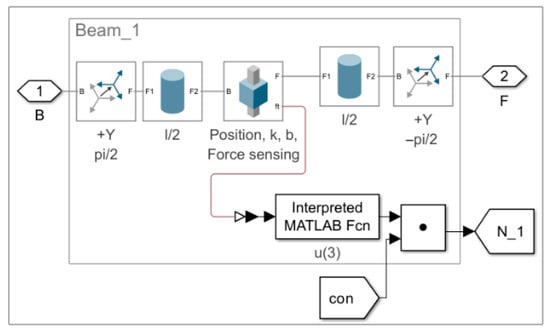
Figure 6. Model 1.3. An illustration of the bar subsystem named Beam_1. The subsystem comprises two solid bodies connected by a prismatic joint with one degree of freedom (1 DOF).

The measurement of nodal displacements δ follows the same principle across all models (Model 1.1, Model 1.2, and Model 1.3). The only difference lies in the (x, y) positioning of the nodes; therefore, only one representative example is shown. Figure 7 presents the subsystem named Node_Deflection_4.

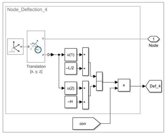
Figure 7. Model 1.1, Model 1.2, and Model 1.3. A detailed view of the deflection measurement subsystem labeled Node_Deflection_4 at coordinates x = −L/2, y = −H.

“Transform Sensor”—Translation [x, y, z] are employed to measure the displacement relative to the World Frame. The remaining blocks are used to isolate the vector components x, y corresponding to displacement in the plane relative to the original position.

Figure 8 presents the subsystem responsible for applying the external load F_load, including its proportional correction via a multiplication constant con. This configuration is identical across all models (Model 1.1, Model 1.2, and Model 1.3).

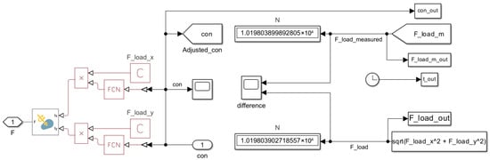
Figure 8. Model 1.1, Model 1.2, and Model 1.3. The subsystem under application of the external load F_load, including its proportional adjustment via the multiplication constant con.

2.2. Example 2: Three Modeling Variants

Figure 9 presents a schematic of the second truss system. The structure is also experimentally modeled using three different approaches:

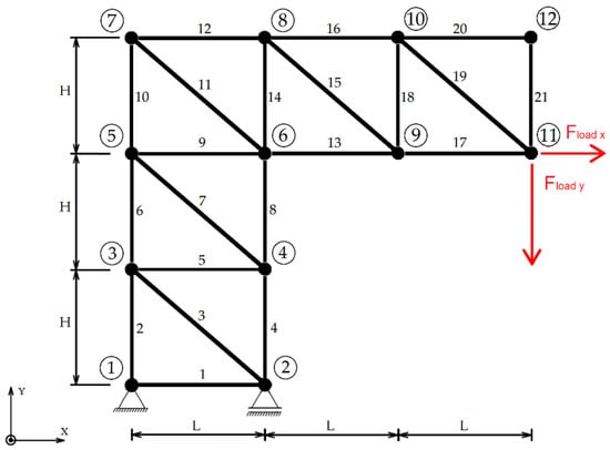
Figure 9. Example 2. A schematic of the truss system subjected to a force vector F_load at Node_11.

• Model 2.1 consists of Euler–Bernoulli beams and joints.
• Model 2.2 is primarily experimental. It is composed of Euler–Bernoulli beams and solid joints. This model does not satisfy the assumptions of the theoretical model, as the nodes do not contain movable joints.
• Model 2.3 comprises solid bars with one degree of freedom (1 DOF) and joints.

The truss system is subjected to an external load applied at Node_11. All bars have an identical cross-section.

2.2.1. Model 2.1: Truss System Composed of Euler–Bernoulli Beams and Joints

Model 2.1, implemented using Simscape Multibody, is presented in Figure 10. The fully assembled functional models are available in [18]. The same block configuration is applied in both Model 2.2 and Model 2.3.

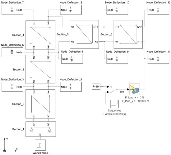
Figure 10. Model 2.1, Model 2.2, and Model 2.3. The structure of the truss system subjected to the force vector F_load at Node_11, implemented in MATLAB–Simscape Multibody, based on the schematic shown in Figure 9.

The truss bar subsystem, based on the Euler–Bernoulli beam model, is analogous to the configuration used in Model 1.1 and Model 1.2 (see Figure 3), and follows the same modeling principles. All the truss bars have an identical structural composition, and only axial force is taken into account.

Figure 11 presents the primary sections, i.e., subsystems of the structure, including those repeated throughout the model. All the components associated with the nodes are consistently labeled as Node_1, Node_2, and so forth.

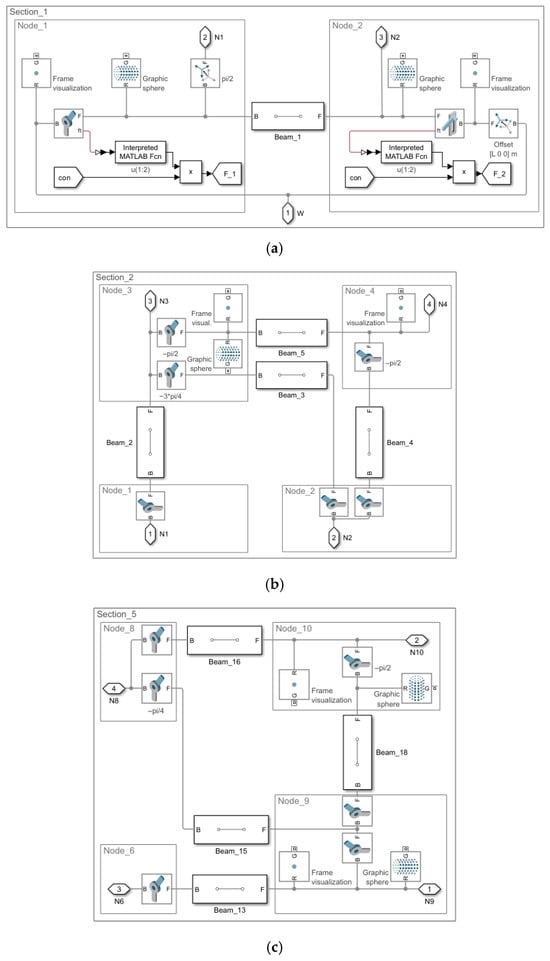
Figure 11. Model 2.1 and Model 2.3. Subsystem types by section: (a) Section_1; (b) Sections_2 to _4 are conceptually identical; (c) Sections_5 to _6 are conceptually identical.

The control measurement of the load force F_{load m} is depicted in Figure 12.

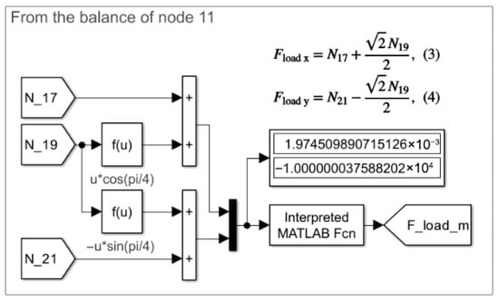
Figure 12. Model 2.1, Model 2.2, and Model 2.3. Measurement of the F_{load m} force in Section_6.

The load force F_{load m} also serves here as a control verification of the computed load force F_load. The value of F_{load m} is derived from the internal forces within the system, specifically from the equilibrium condition at Node_11.

$$\sum F_x=0; F_{\mathrm{l}\mathrm{o}\mathrm{a}\mathrm{d} x}-N_{17}-{\displaystyle \frac{\sqrt{2}{·N}_{19}}{2}}=0$$

(3)

$$\sum F_y=0; F_{\mathrm{l}\mathrm{o}\mathrm{a}\mathrm{d} y}-N_{21}+{\displaystyle \frac{\sqrt{2}{·N}_{19}}{2}}=0$$

(4)

The F_load force represents the external load applied to the system. In cases where multiple external forces act on the structure, the one with the maximum magnitude is selected for control measurement.

2.2.2. Model 2.2. Truss System Composed of Euler–Bernoulli Beams and Solid Joints

The block configuration of Model 2.2, constructed in Simscape Multibody, is identical to the configuration shown in Figure 10. The only difference lies in the implementation of the nodes.

The subsystem of the truss bar, based on the Euler–Bernoulli beam model, is analogous to that used in Model 1.1 and Model 1.2 (see Figure 3). The same modeling principles apply. All truss bars in the simulation are structurally identical, and only axial force is considered.

The subsequent illustration, Figure 13, presents the primary structural sections—the subsystems that define the construction and those that are repeated. All the elements associated with the nodes are labeled consistently as Node_1, Node_2, etc. Section_1, shown in Figure 11a, remains the same across Model 2.1, Model 2.2, and Model 2.3.

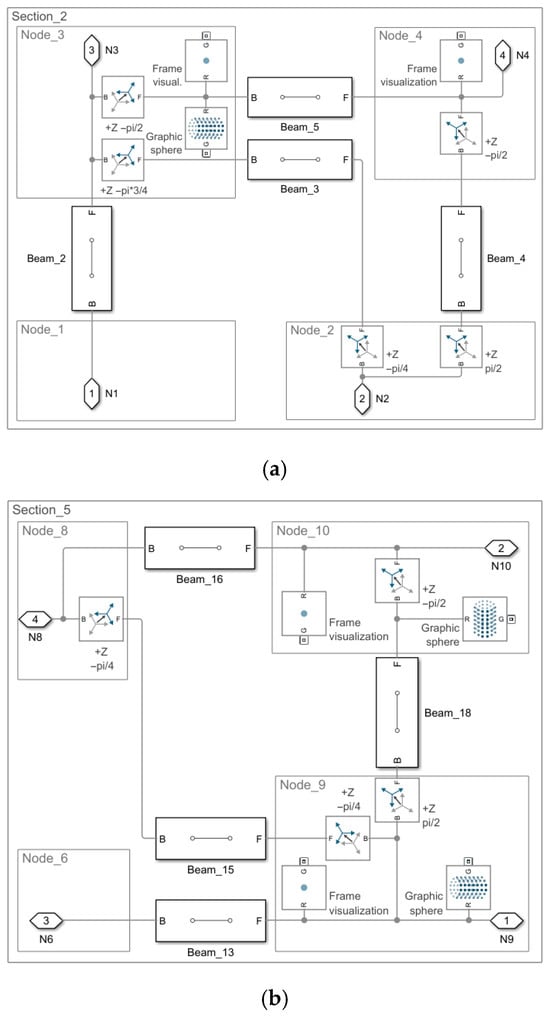
Figure 13. Model 2.2. The conceptual structure of the subsystems by section: (a) Sections_2 to _4 share an identical configuration; (b) Sections_5 to _6 are conceptually identical.

The control measurement of the load force F_{load m} is identical to that in Model 2.1, as shown in Figure 12. Equations (3) and (4) apply. However, this interpretation is not entirely accurate in this particular case, as the nodes do not contain movable joints. Nevertheless, it is sufficient for the intended purpose.

2.2.3. Model 2.3. Truss System Composed of Solid Bars with 1 DOF and Joints

The configuration of Model 2.3, assembled in Simscape Multibody, has the same block structure as that shown in Figure 10. The only difference lies in the representation of the bars, which is analogous to that used in Model 1.3; see Figure 6. The bar consists of two rigid bodies connected by a prismatic joint with one degree of freedom (1 DOF). Within the joint, the stiffness k is defined as ES/l, along with the damping b and the initial position set to zero. All the truss bars in the simulation model (Model 2.3) have an identical structure.

The measurement of node displacements is consistent across all three models (Model 2.1, Model 2.2, and Model 2.3); the nodes differ only in their (x, y) locations. The concept is identical to that for the structure shown in Figure 7.

The subsystem used to define the F_load force is identical to that shown in Figure 8, and is shared by all three models (Model 2.1, Model 2.2, and Model 2.3).

3. Computational Optimization Procedure

The optimization consists of identifying the appropriate input level—specifically, the value of the ratio F_load/con for a given model—at which the computational accuracy is maximized. The gain in precision can reach two to three orders of magnitude. The resulting values will be compared against the theoretical solutions obtained for Models 1.1, 1.2, and 1.3, and against the more complex structures represented by Models 2.1, 2.2, and 2.3. Additionally, a more complex test configuration derived from Model 1.1 will be evaluated to further assess its potential for improving the accuracy larger structural systems, considering both computational precision and processing time. The optimization is performed by applying a stepwise change (scaling) in the proportionality constant con. Alternatively, a dynamic adjustment of con based on the difference between F_load and F_{load m} may be implemented. In such cases, the value of con is determined proportionally to F_load. Suitable computational solvers for this type of simulation within the toolbox include ode15s, ode23s, ode23t, and ode23tb (see [22] for further details). Among these, ode15s was selected for its proven reliability and computational efficiency. Another option for stiff systems is also solvers ode23s, ode23t, and ode23tb. The solvers ode45, ode23, and ode113 are not recommended for stiff systems (longer computational times).

The following Procedure 1 describes a simple algorithm for selecting the control measurement of the load force F_{_load_m}. The entire set of measurements indexed by i is divided into time sequences, denoted as Sequence, with a total number k. During each sequence, the data F_{_load_m_separ_k} is selected outside the transient state Lag, caused by the natural vibration delay of the system. That is, to process the mean value Mean_F_{_load_m}(k) from the given measurement sequence, data from the steady-state condition is used. This continues until a step change in the F_{_load_m} force occurs, at which point the end of the sequence yields undesired results. These are separated in advance using Lead. The proportionality of the step change in the load force F_{_load_m} is realized using the multiplication constant con. Additionally, the maximum Max_F_{_load_m}(k) and minimum Min_F_{_load_m}(k) are computed for each sequence.

The results are subsequently visualized in the plot F_{_load_m} = function(con), as shown in Figure 14, Figure 15 and Figure 16. The closer the value of F_{_load_m} is to the applied force F_{_load}, the more accurate the computation is, provided that the variation in F_{_load_m} remains minimal. If the variation in F_{_load_m} exceeds the maximum and minimum values observed in the preceding sequence, the resulting error may increase (depending on the sample). In such cases, it is not meaningful to proceed with the computation.

Procedure 1: Visualization of the computational accuracy of Fload m as a function of con
	Input: multiplication constant con, vector of load force F_load, control measurement of the load force F_load_m, simulation sequence duration SampleTime, measurement sequence (Sequence), end of simulation StopTime, vector of sequences Seq_vector, Lag, Lead, sequence step k, ith sample of the F_load_m variable.
	Output: Sorted values F_load_m_separ_k, maxima of the measured values for the given sequence Max_F_load_m(k), minima of the measured values for the given sequence Min_F_load_m(k), mean of the measured values for the given sequence Mean_F_load_m(k), time for all sequences TIME{k}.
1	For k = 1 to size(Seq_vector) do
2	If k < size(Seq_vector) then
3	For i = 1 to size(F_load_m) do
4	If ((Seq_vector(k)-Lag) ≤ F_load_m(i)) & (F_load_m(i) ≤ (Seq_vector(k+1)-Lead))
5	F_load_m_separ (i) ← F_load_m (i)
6	End
7	End
8	F_load_m_separ_k← F_load_m_separ
9	clear F_load_m_separ—delete previous values
10	F_load_m_separ_1 = F_load_m_separ_k(1,:)—force vector extracted from matrix        F_load_m_separ_k for the sequence
11	F_load_m_separ_2 = F_load_m_separ_k(2,:)—time vector extracted from matrix        F_load_m_separ_k for the sequence
12	A{k} = F_load_m_separ_1(F_load_m_separ_1 ~=0)—exclusion of invalid values
13	Max_F_load_m(k) = max(A{k})—maxima of F_load_m_separ_k
14	Min_F_load_m(k) = min(A{k})—minima of F_load_m_separ_k
15	Mean_F_load_m(k)—mean values computed from F_load_m_separ_ 1
16	time = F_load_m_separ_2 (F_load_m_separ_2 ~= 0)—exclusion of invalid time values        for the sequence
17	TIME{k}—all time sequences
18	Else
19	End
20	End

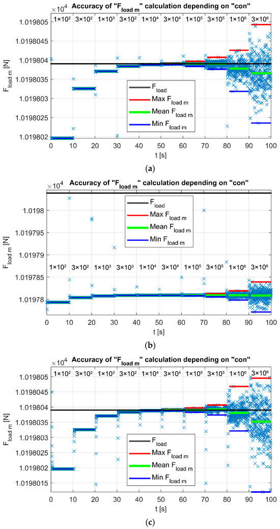
Figure 14. The computational accuracy of the control measurement of the load force F_{load m}. The closer the value of F_{load_m} is to the force F_{_load}, the more accurate the computation is, provided that the swing of F_{load_m} values remains minimal: (a) Model 1.1; (b) Model 1.2; (c) Model 1.3.

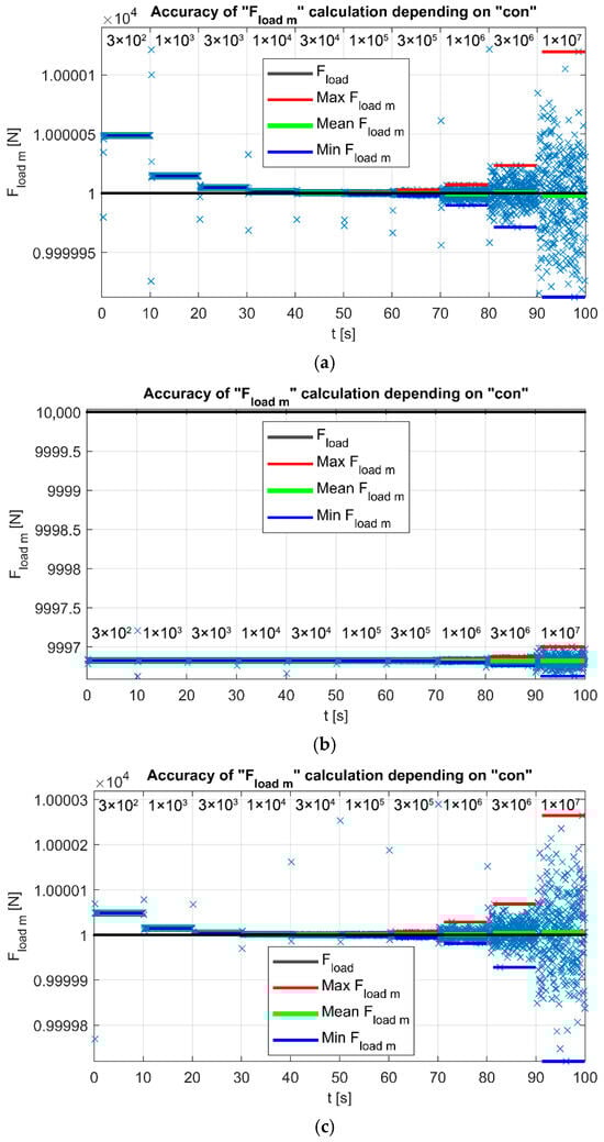
Figure 15. The computational accuracy of the control measurement of the load force F_{load m}. The closer the value of F_{_load_m} is to the force F_{_load}, the more accurate the computation is, provided that the swing of F_{_load_m} values remains minimal: (a) Model 2.1; (b) Model 2.2; (c) Model 2.3.

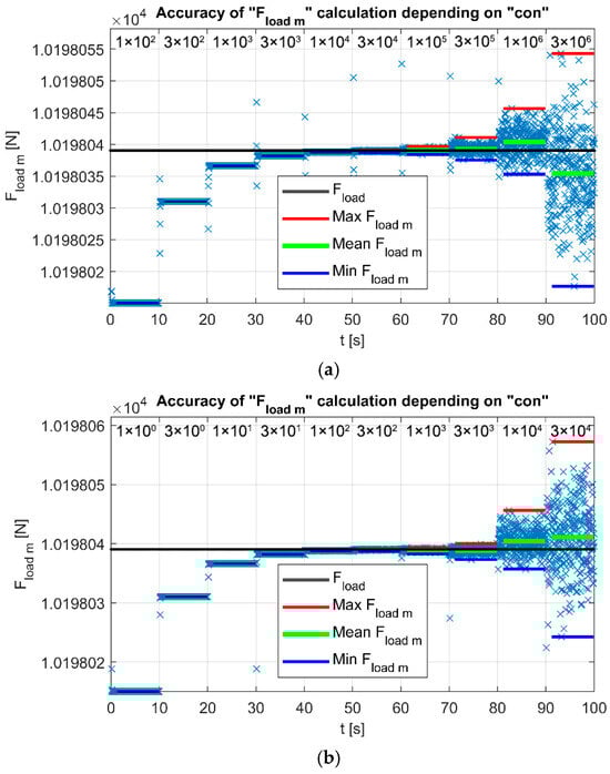
Figure 16. The computational accuracy of the control measurement of the load force F_{load m} for Example 3. This represents a test computation of a more complex structure consisting of 39 bars, created based on Model 1.1 from Example 2. The closer the value of F_{_load_m} is to the force F_{_load}, the more accurate the computation is, provided that the swing of F_{_load_m} values remains minimal: (a) bar diameter d = 0.01 m; (b) bar diameter d = 0.1 m.

The output plots below illustrate the computational accuracy of the control measurement of the load force F_{load m} as a function of the proportionality constant con for (a) Model 1.1, (b) Model 1.2, and (c) Model 1.3.

The output plots below illustrate the computational accuracy of the control measurement of the load force F_{load m} as a function of the proportionality constant con for (a) Model 2.1, (b) Model 2.2, and (c) Model 2.3.

The output plots below illustrate the computational accuracy of the control measurement of the load force F_{load m} as a function of the proportionality constant con. A more complex test variant, created based on Model 1.1 from Example 2, was used. A total of 39 bars were implemented.

The results indicate that for different multiples of the load force vector F_load, the computational accuracy also varies. A similar situation occurs when other parameters are changed, such as the bar diameter, Young’s modulus, or similar material properties. Our objective was to investigate all factors influencing this computation and to explore how such optimization could be standardized for future analyses. In the script “Dependence_Floadm_on_con.m” [18], we initially planned to calculate the standard deviation [23] in addition to the mean and extreme values; however, this approach proved to be impractical for the following reasons:

• The computation did not consistently conform 100% to the theoretical probability of the Gaussian distribution [24]. For example, instead of the expected 99.73% probability set, the actual result was 98.98%.
• During the computation, the simulation can be interrupted at any moment. As a result, no samples are excluded, and calculating the standard deviation does not provide meaningful insight in this context. Consequently, even samples that fall outside multiples of the standard deviation interval remain included in the data set. Therefore, we opted to use the actual maxima and minima derived from the given set of values.

4. Results

Analytical solutions were obtained using publicly available scripts from [25] for various truss systems analyzed through Matrix Structural Analysis in the MATLAB environment. Essentially, these involve two-dimensional problems derived from the principles of the Finite Element Method (FEM) [26] or, for example, [27] (pp. 141–143). Specific examples were selected or created for testing in Simscape Multibody, with the aim of achieving the highest possible computational accuracy. Additionally, we were interested in exploring how load visualization can be implemented in this toolbox. Load visualization is a representation of a system with bars deformation due to load (Figure 17 and Figure 18). Within each example, the individual models differ slightly, either in the configuration of the bars or in the design of the nodes.

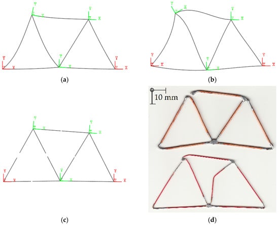
Figure 17. Deformed state visualization across the models: (a) Model 1.1; (b) Model 1.2; (c) Model 1.3 (Young’s modulus E reduced by three orders of magnitude); (d) two physical models with cross-sectional areas of S₁ = 1.1309 mm² and S₂ = 0.3848 mm².

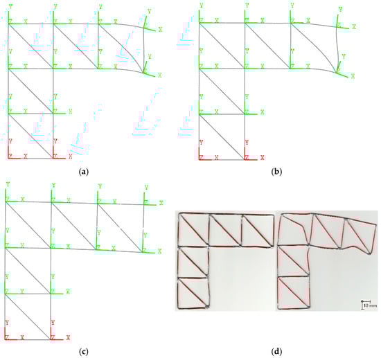
Figure 18. Visualization of the deformed state in the structural models: (a) Model 2.1; (b) Model 2.2; (c) Model 2.3 (Young’s modulus, E, reduced by three orders of magnitude); (d) Two physical structures with different cross–sectional areas of the bars, S₁ = 1.5393 mm² and S₂ = 0.7853 mm².

The outputs from Models 1.1, 1.2, and 1.3 in Example 1, as well as Models 2.1, 2.2, and 2.3 in Example 2, obtained through simulations in MATLAB–Multibody and from theoretical calculations, are summarized in the following tables: Table 1 and Table 2. These outputs also include visualizations of the deformed state. Additionally, Table 3 presents a case involving an extended version of Model 1.1 with a larger number of bars. For this extended model, analytical solution formulas were not included; the results are provided only in numerical form.

Table 1. A comparison of the theoretical results for forces N₁–N₇ acting in the bars, forces F₁, F₃ (not reactions) at the supports of Node_1 and Node_3, and the deflections δ₂, δ₄, and δ₅, with the results from the individual models Model 1.1, Model 1.2, and Model 1.3 constructed in MATLAB–Multibody. The simulation time for the optimal con ranges from 2 to 5 s. Hardware configuration: processor i9–10900, 2.8 GHz, 32 GB RAM, MATLAB 2024a, 64-bit. The same solver (ode15s) was used across all models, with identical settings for absolute and relative tolerances (10⁻³) and a maximum iteration step of 0.01 within a variable step.

Quantity [Unit]	Theoretical Calculation	MATLAB Model 1.1	MATLAB Model 1.2	MATLAB Model 1.3
N1 [N]	−0.94337567·103	−0.94337566·103	−0.94322189·103	−0.94337567·103
N2 [N]	0.94337567·103	0.94337562·103	0.94322214·103	0.94337563·103
N3 [N]	1.88675134·103	1.88675121·103	1.88649462·103	1.88675121·103
N4 [N]	9.66025403·103	9.66025400·103	9.65990727·103	9.66025394·103
N5 [N]	1.88675134·103	1.88675131·103	1.88681570·103	1.88675120·103
N6 [N]	−1.88675134·103	−1.88675129·103	−1.88620302·103	−1.88675108·103
N7 [N]	1.88675134·103	1.88675124·103	1.88657522·103	1.88675128·103
F1x [N]	3.88675134·103	3.88675125·103	3.88666800·103	3.88675120·103
F1y [N]	8.36602540·103	8.36602540·103	8.36602543·103	8.36602535·103
F3x [N]	−1.88675134·103	−1.88675122·103	−1.88666800·103	−1.88675126·103
F3y [N]	1.63397459·103	1.63397452·103	1.63397457·103	1.63397461·103
FLoad x 1 [N]	2.00000000·103	2.00000012·103	2.00005115·103	2.00000015·103
FLoad y 1 [N]	10.00000000·103	9.99999994·103	9.99975543·103	9.99999980·103
δ2x [m]	−0.57197295·10−4	−0.57197293·10−4	−0.57187981·10−4	−0.57197300·10−4
δ2y [m]	4.70248778·10−4	4.70248791·10−4	4.70200032·10−4	4.70248768·10−4
δ4x [m]	0.35464965·10−4	0.35464940·10−4	0.35486893·10−4	0.35464980·10−4
δ4y [m]	6.55838856·10−4	6.55838876·10−4	6.55801902·10−4	6.55838846·10−4
δ5x [m]	1.49859556·10−4	1.49859564·10−4	1.49865932·10−4	1.49859564·10−4
δ5y [m]	2.18612952·10−4	2.18612977·10−4	2.18604317·10−4	2.18612957·10−4

¹ Verification of the calculated magnitude of the load force F_Load based on the equilibrium of Node_4, according to Equations (1) and (2), used solely for the optimization of the multiplication constant con.

Table 2. A comparison of the theoretical results for the forces N₁–N₂₁ acting in the bars, forces F₁ and F₂ (not reactions) at the supports of Node_1 and Node_2, and displacements δ₂–δ₁₂. These results are compared with those obtained from Models 2.1, 2.2, and 2.3 simulated in MATLAB–Multibody. The simulation time for the optimal con value ranged from 10 to 22 s. The calculations were performed on a processor i9–10900, 2.8 GHz, with 32 GB RAM, using MATLAB 2024a, 64-bit. The same solver (ode15s) and identical settings for absolute tolerance, relative tolerance (10⁻³), and the maximum iteration step (0.01) within the variable–step configuration were used throughout.

Quantity [Unit]	Theoretical Calculation	MATLAB Model 2.1	MATLAB Model 2.2	MATLAB Model 2.3
N1 [N]	0	−0.00036038	0.06985929	−0.00092453
N2 [N]	2·104	2.00000007·104	1.99997963·104	2.00000012·104
N3 [N]	0	−0.00030489	−0.70545982	−0.00057530
N4 [N]	−3·104	−3.00000005·104	−2.99992002·104	−3.00000008·104
N5 [N]	0	−0.00069505	0.41597051	−0.00181315
N6 [N]	2·104	2.00000004·104	1.99999088·104	2.00000008·104
N7 [N]	0	−0.00084519	−3.72374373	−0.00178803
N8 [N]	−3·104	−2.99999998·104	−2.99971831·104	−2.99999994·104
N9 [N]	0	−0.00123336	−1.59349130	−0.00281782
N10 [N]	2·104	1.99999997·104	1.99947667·104	1.99999993·104
N11 [N]	−2.82842712·104	−2.82842702·104	−2.82719856·104	−2.82842694·104
N12 [N]	2·104	1.99999997·104	1.99945650·104	1.99999998·104
N13 [N]	−2·104	−1.99999982·104	−1.99954651·104	−1.99999958·104
N14 [N]	−1·104	−1.00000023·104	−1.00000467·104	−1.00000050·104
N15 [N]	1.41421356·104	1.41421358·104	1.41343004·104	1.41421362·104
N16 [N]	1·104	9.99999991·103	1.00014635·104	9.99999993·103
N17 [N]	−1·104	−9.99999820·103	−9.99855709·103	−9.99999543·103
N18 [N]	−1·104	−1.00000000·104	−9.99689885·103	−1.00000002·104
N19 [N]	1.41421356·104	1.41421358·104	1.41391288·104	1.41421366·104
N20 [N]	0	0.00019897	1.13419678	0.00002046
N21 [N]	0	−0.00019154	1.04655832	0.00011316
F1x [N]	0	−0.00001027	−0.00000029	−0.00008829
F1y [N]	2·104	2.00000007·104	2.00001212·104	2.00000012·104
F2x [N]	0	0	0	0
F2y [N]	−3·104	−3.00000007·104	−3.00001212·104	−3.00000012·104
FLoad x 1 [N]	0	0.00197450	−0.68322370	0.00527883
FLoad y 1 [N]	−1·104	−1.00000003·104	−9.99682731·103	−1.00000005·104
δ2x [m]	0	0	0	0
δ2y [m]	0	0	0	0
δ3x [m]	1.21260909·10−3	1.21260907·10−3	1.21268896·10−3	1.21260919·10−3
δ3y [m]	1.21260909·10−3	1.21260913·10−3	1.21259634·10−3	1.21260913·10−3
δ4x [m]	1.21260909·10−3	1.21260901·10−3	1.21269939·10−3	1.21260893·10−3
δ4y [m]	−1.81891363·10−3	−1.81891360·10−3	−1.81886655·10−3	−1.81891370·10−3
δ5x [m]	5.45674090·10−3	5.45674098·10−3	5.45724232·10−3	5.45674144·10−3
δ5y [m]	2.42521818·10−3	2.42521815·10−3	2.42517526·10−3	2.42521798·10−3
δ6x [m]	5.45674090·10−3	5.45674070·10−3	5.45710518·10−3	5.45674065·10−3
δ6y [m]	−3.63782727·10−3	−3.63782731·10−3	−3.63763418·10−3	−3.63782759·10−3
δ7x [m]	1.61621718·10−2	1.61621718·10−2	1.61606005·10−2	1.61621722·10−2
δ7y [m]	3.63782727·10−3	3.63782650·10−3	3.63730639·10−3	3.63782513·10−3
δ8x [m]	1.737478098·10−2	1.737478055·10−2	1.73728087·10−2	1.73747803·10−2
δ8y [m]	−4.24413181·10−3	−4.24413292·10−3	−4.24416919·10−3	−4.24413480·10−3
δ9x [m]	4.24413181·10−3	4.24413010·10−3	4.24443048·10−3	4.24412783·10−3
δ9y [m]	−1.908966920·10−2	−1.90896690·10−2	−1.90858478·10−2	−1.90896690·10−2
δ10x [m]	1.798108552·10−2	1.79810834·10−2	1.79788210·10−2	1.79810809·10−2
δ10y [m]	−1.969597374·10−2	−1.96959748·10−2	−1.96922747·10−2	−1.96959767·10−2
δ11x [m]	3.63782727·10−3	3.63782379·10−3	3.63775137·10−3	3.63781893·10−3
δ11y [m]	−3.575412022·10−2	−3.57541196·10−2	−3.57470982·10−2	−3.57541193·10−2
δ12x [m]	1.798108552·10−2	1.79810817·10−2	1.797846122·10−2	1.79810766·10−2
δ12y [m]	−3.575412022·10−2	−3.57541210·10−2	−3.574737653·10−2	−3.57541227·10−2

¹ Verification of the loading force F_Load magnitude based on Node_11 equilibrium, according to Equations (3) and (4), used solely for optimizing the multiplication constant con.

Table 3. Example 3. A comparison of the theoretical results for forces N₁–N₃₉ acting in the bars, as well as forces F_1L, F_20R (not reactions) at the supports of nodes Node_1 and Node_20, and deflections δ₂–δ₁₉ and δ₂₁, with the results from the MATLAB–Simscape Multibody model. The simulation time for the optimal value of con was 94 s. Hardware specifications: Processor i9–10900, 2.8 GHz, 32 GB RAM, Matlab 2024a, 64-bit. The same solver (ode15s) was used, with identical settings for absolute and relative tolerances (10⁻³), and a maximum iteration step size of 0.01 within a variable step.

Quantity [Unit]	Theoretical Calculation	MATLAB Example 3	Quantity [Unit]	Theoretical Calculation	MATLAB Example 3
N1 [N]	1.11696551·104	1.11696549·104	F20Ry [N]	−0.03267949·104	0.03267948·104
N2 [N]	0.03773502·104	0.03773502·104	FLoadx 1 [N]	0.2·104	0.20000003·104
N3 [N]	−0.16980762·104	−0.16980761·104	FLoady 1 [N]	1·104	0.99999997·104
N4 [N]	0.33961524·104	0.33961518·104	δ2x [m]	−0.10295513·10−3	−0.10295517·10−3
N5 [N]	−0.03773502·104	−0.03773503·104	δ2y [m]	1.63899678·10−3	1.63899669·10−3
N6 [N]	0.03773502·104	0.03773502·104	δ3x [m]	−0.81654806·10−3	−0.81654804·10−3
N7 [N]	−0.13207259·104	−0.13207258·104	δ3y [m]	1.25342200·10−3	1.25342194·10−3
N8 [N]	0.30188021·104	0.30188015·104	δ4x [m]	−0.18303134·10−3	−0.18303137·10−3
N9 [N]	−0.03773502·104	−0.03773502·104	δ4y [m]	2.12614960·10−3	2.12614946·10−3
N10 [N]	0.03773502·104	0.03773502·104	δ5x [m]	−0.61063780·10−3	−0.61063780·10−3
N11 [N]	−0.09433756·104	−0.09433756·104	δ5y [m]	1.90568920·10−3	1.90568908·10−3
N12 [N]	0.26414518·104	0.26414514·104	δ6x [m]	−0.24022864·10−3	−0.24022866·10−3
N13 [N]	−0.03773502·104	−0.03773502·104	δ6y [m]	2.32270114·10−3	2.32270096·10−3
N14 [N]	0.03773502·104	0.03773502·104	δ7x [m]	−0.42760645·10−3	−0.42760645·10−3
N15 [N]	−0.05660254·104	−0.05660253·104	δ7y [m]	2.24093681·10−3	2.24093665·10−3
N16 [N]	0.22641016·104	0.22641010·104	δ8x [m]	−0.27454701·10−3	−0.27454702·10−3
N17 [N]	−0.03773502·104	−0.03773501·104	δ8y [m]	2.28148798·10−3	2.28148782·10−3
N18 [N]	0.03773502·104	0.03773501·104	δ9x [m]	−0.26745402·10−3	−0.26745405·10−3
N19 [N]	−0.01886751·104	−0.01886751·104	δ9y [m]	2.31200143·10−3	2.31200128·10−3
N20 [N]	0.18867513·104	0.18867509·104	δ10x [m]	−0.28598647·10−3	−0.28598646·10−3
N21 [N]	−0.03773502·104	−0.03773502·104	δ10y [m]	2.05534673·10−3	2.05534661·10−3
N22 [N]	0.03773502·104	0.03773502·104	δ11x [m]	−0.13018051·10−3	−0.13018053·10−3
N23 [N]	0.01886751·104	0.01886750·104	δ11y [m]	2.17171965·10−3	2.17171953·10−3
N24 [N]	0.15094010·104	0.15094006·104	δ12x [m]	−0.27454701·10−3	−0.27454697·10−3
N25 [N]	−0.03773502·104	−0.03773502·104	δ12y [m]	1.69711398·10−3	1.69711389·10−3
N26 [N]	0.03773502·104	0.03773501·104	δ13x [m]	−0.01578592·10−3	−0.01578590·10−3
N27 [N]	0.05660254·104	0.05660252·104	δ13y [m]	1.87292807·10−3	1.87292798·10−3
N28 [N]	0.11320508·104	0.11320505·104	δ14x [m]	−0.24022864·10−3	−0.24022858·10−3
N29 [N]	−0.03773502·104	−0.03773501·104	δ14y [m]	1.25962634·10−3	1.25962628·10−3
N30 [N]	0.03773502·104	0.03773503·104	δ15x [m]	0.07572974·10−3	0.07572976·10−3
N31 [N]	0.09433756·104	0.09433753·104	δ15y [m]	1.46846330·10−3	1.46846324·10−3
N32 [N]	0.07547005·104	0.07547003·104	δ16x [m]	−0.18303134·10−3	−0.18303129·10−3
N33 [N]	−0.03773502·104	−0.03773503·104	δ16y [m]	0.79572039·10−3	0.79572037·10−3
N34 [N]	0.03773502·104	0.03773501·104	δ17x [m]	0.14436650·10−3	0.14436654·10−3
N35 [N]	0.13207259·104	0.13207256·104	δ17y [m]	1.01116193·10−3	1.01116192·10−3
N36 [N]	0.03773502·104	0.03773501·104	δ18x [m]	−0.10295513·10−3	−0.10295508·10−3
N37 [N]	−0.03773502·104	−0.03773501·104	δ18y [m]	0.35823274·10−3	0.35823275·10−3
N38 [N]	0.03773502·104	0.03773502·104	δ19x [m]	0.19012433·10−3	0.19012439·10−3
N39 [N]	0.16980762·104	0.16980758·104	δ19y [m]	0.55386056·10−3	0.55386056·10−3
F1Lx [N]	−0.38867513·104	0.38867509·104	δ21x [m]	0.21300325·10−3	0.21300326·10−3
F1Ly [N]	−0.96732050·104	0.96732051·104	δ21y [m]	0.14939578·10−3	0.14939579·10−3
F20Rx [N]	0.18867513·104	−0.18867508·104

¹ Verification of the calculation of the load force magnitude F_Load based on the equilibrium of Node_3 and Equations (51) and (52). This serves solely for the optimization of the multiplication constant con.

4.1. Results for Example 1

4.1.1. Theoretical Calculation for Example 1: Three Modeling Variants

Table 1 summarizes a comparison of the individual results for Models 1.1, 1.2, and 1.3 obtained from MATLAB–Multibody and from the theoretical calculation.

The following analytical expressions were obtained from the symbolic computation performed for Example 1. The force vectors, which do not represent reactions, at the supports of Node_1 and Node_3 are calculated as follows:

$${\mathbf{F}}_1=\left[\begin{array}{c}{\displaystyle \frac{2\hspace{0.17em}{F}_x\hspace{0.17em}H+F_y\hspace{0.17em}L}{4\hspace{0.17em}H}}\\ {\displaystyle \frac{2\hspace{0.17em}{F}_x\hspace{0.17em}H+3\hspace{0.17em}{F}_y\hspace{0.17em}L}{4\hspace{0.17em}L}}\end{array}\right]$$

(5)

$${\mathbf{F}}_3=\left[\begin{array}{c}{\displaystyle \frac{2\hspace{0.17em}{F}_x\hspace{0.17em}H-F_y\hspace{0.17em}L}{4\hspace{0.17em}H}}\\ -{\displaystyle \frac{2\hspace{0.17em}{F}_x\hspace{0.17em}H+F_y\hspace{0.17em}L}{4\hspace{0.17em}L}}\end{array}\right]$$

(6)

The forces in the bars are derived as follows:

$$N_1={\displaystyle \frac{2\hspace{0.17em}{F}_x\hspace{0.17em}H-F_y\hspace{0.17em}L}{8\hspace{0.17em}H}}$$

(7)

$$N_2=-{\displaystyle \frac{2\hspace{0.17em}{F}_x\hspace{0.17em}H-F_y\hspace{0.17em}L}{8\hspace{0.17em}H}}$$

(8)

$$N_3=-{\displaystyle \frac{2\hspace{0.17em}{F}_x\hspace{0.17em}H-F_y\hspace{0.17em}L}{4\hspace{0.17em}H}}$$

(9)

$$N_4={\displaystyle \frac{\sqrt{4\hspace{0.17em}{H}^2+L^2}\hspace{0.17em}\left(2\hspace{0.17em}{F}_x\hspace{0.17em}H+3\hspace{0.17em}{F}_y\hspace{0.17em}L\right)}{8\hspace{0.17em}H\hspace{0.17em}L}}$$

(10)

$$N_5=-{\displaystyle \frac{\sqrt{4\hspace{0.17em}{H}^2+L^2}\hspace{0.17em}\left(2\hspace{0.17em}{F}_x\hspace{0.17em}H-F_y\hspace{0.17em}L\right)}{8\hspace{0.17em}H\hspace{0.17em}L}}$$

(11)

$$N_6={\displaystyle \frac{\sqrt{4\hspace{0.17em}{H}^2+L^2}\hspace{0.17em}\left(2\hspace{0.17em}{F}_x\hspace{0.17em}H-F_y\hspace{0.17em}L\right)}{8\hspace{0.17em}H\hspace{0.17em}L}}$$

(12)

$$N_7=-{\displaystyle \frac{\sqrt{4\hspace{0.17em}{H}^2+L^2}\hspace{0.17em}\left(2\hspace{0.17em}{F}_x\hspace{0.17em}H-F_y\hspace{0.17em}L\right)}{8\hspace{0.17em}H\hspace{0.17em}L}}$$

(13)

The displacement vectors δ of the node displacements Node_2, Node_4, and Node_5 are calculated as follows:

$${\mathsf{\delta }}_2=\left[\begin{array}{c}{\displaystyle \frac{L\hspace{0.17em}\left(2\hspace{0.17em}{F}_x\hspace{0.17em}H-F_y\hspace{0.17em}L\right)}{8\hspace{0.17em}E S\hspace{0.17em}H}}\\ {\displaystyle \frac{F_y\hspace{0.17em}{\left(4\hspace{0.17em}{H}^2+L^2\right)}^{3/2}+2\hspace{0.17em}{F}_y\hspace{0.17em}{L}^3-4\hspace{0.17em}{F}_x\hspace{0.17em}H\hspace{0.17em}{L}^2}{16\hspace{0.17em}E S\hspace{0.17em}{H}^2}}\end{array}\right]$$

(14)

$${\mathsf{\delta }}_4=\left[\begin{array}{c}{\displaystyle \frac{F_x\hspace{0.17em}\left(8\hspace{0.17em}{\left(H^2+\frac{L^2}{4}\right)}^{3/2}+3\hspace{0.17em}{L}^3\right)}{8\hspace{0.17em}E S\hspace{0.17em}\hspace{0.17em}{L}^2}}-{\displaystyle \frac{3\hspace{0.17em}{F}_y\hspace{0.17em}{L}^2}{16\hspace{0.17em}E S\hspace{0.17em}\hspace{0.17em}H}}\\ {\displaystyle \frac{3\hspace{0.17em}{F}_y\hspace{0.17em}{\left(4\hspace{0.17em}{H}^2+L^2\right)}^{3/2}+3\hspace{0.17em}{F}_y\hspace{0.17em}{L}^3-6\hspace{0.17em}{F}_x\hspace{0.17em}H\hspace{0.17em}{L}^2}{32\hspace{0.17em}E S\hspace{0.17em}\hspace{0.17em}{H}^2}}\end{array}\right]$$

(15)

$${\mathsf{\delta }}_5=\left[\begin{array}{c}{\displaystyle \frac{F_x\hspace{0.17em}\left(8\hspace{0.17em}{\left(H^2+\frac{L^2}{4}\right)}^{3/2}-L^3\right)}{8\hspace{0.17em}E S\hspace{0.17em}\hspace{0.17em}{L}^2}}+{\displaystyle \frac{F_y\hspace{0.17em}{L}^2}{16\hspace{0.17em}E S\hspace{0.17em}\hspace{0.17em}H}}\\ {\displaystyle \frac{F_y\hspace{0.17em}{\left(4\hspace{0.17em}{H}^2+L^2\right)}^{3/2}+F_y\hspace{0.17em}{L}^3-2\hspace{0.17em}{F}_x\hspace{0.17em}H\hspace{0.17em}{L}^2}{32\hspace{0.17em}E S\hspace{0.17em}\hspace{0.17em}{H}^2}}\end{array}\right]$$

(16)

For all modeling variants—Model 1.1, Model 1.2, and Model 1.3—the force vector F_load = [F_x, F_y]^T has the numerical value F_load = [2, 10]^T kN. The lengths of the bars are determined by the distances between the nodes or by the dimensions of the system, with L = 1 m and H = L∙cos(π/6) m. The bars have identical diameters of d = 0.01 m. The Young’s modulus E is 210 GPa.

For Models 1.1 and 1.2, the shear modulus G is 79 GPa, and the material density (Density) is 7800 kg/m³. Poisson’s ratio is 0.28. The values for proportional (Rayleigh) damping are kept at their default settings for practical purposes, with b_m = 0.01 s⁻¹ and b_k = 0.01 s. Essentially, these values can be set to nearly zero. The damping at the supports is b_rj = 1 N∙m∙s∙rad⁻¹.

For Model 1.3, the damping at the supports is b_rj = 6∙10⁴ N∙m∙s∙rad⁻¹. The damping in the bars is b = 10 N∙s∙m⁻¹. The axial stiffness of the bars under tension/compression is defined as k = E∙π∙d²∙(4∙l)⁻¹ N∙s∙m⁻¹.

4.1.2. Results for Example 1: Theoretical Calculation and MATLAB Models

For clarity, the results are presented in the Table 1, with the theoretical calculations listed first, followed by those from the individual models.

After optimization, Model 1.1 achieved guaranteed accuracy up to six decimal places compared to the theoretical model. Model 1.3 performed similarly. Model 1.2 attained guaranteed accuracy of approximately two to three decimal places, despite not fulfilling the assumptions of the theoretical model. In its nodes, there are no movable joints.

4.1.3. Results for Example 1: Visualization of the Deformed State of the Models

The visualization of the deformed state was performed for a specified norm of the displacement vector, ||δ₄|| = 0.1 m, at Node_4; see, for example, Figure 1. This value is not critical, and serves solely to produce an exaggerated depiction of the deformation in theoretical models. For the material used in the physical model, copper (Cu) was selected due to its favorable ductility and plasticity. The bars had uniform diameters within each sample: d_a = 1.2∙10⁻³ m in the first case and d_b = 0.7∙10⁻³ m in the second. The dimensions were L = 40∙10⁻³ m, H = L∙cos(π/6) m. The model was constructed exclusively for the purpose of testing excessive deformation. In the theoretical models, the material was not changed, as it did not influence the resulting deformed shape.

For Model 1.3, the stiffness of the bars under uniaxial tension/compression needs to be reduced by approximately three orders of magnitude, calculated as k = 10⁻³∙E∙π∙d²∙(4∙l)⁻¹ N∙s∙m⁻¹.

The various models exhibit differences in the excessively deformed state when compared to the physical structure shown in Figure 17d. The best agreement with the physical structure was achieved by Model 1.1 in Figure 17a and Model 1.3 in Figure 17c. In the physical structure, the results are influenced by manufacturing precision and the method of applying support and load. Model 1.1 provided even better agreement when lower damping values b_rj were applied in the joints at the supports, combined with higher damping coefficients b_k in the bars. This allowed the force effect from the load point to be transmitted more effectively throughout the structure. However, this model entailed the disadvantage of increased computational time required for analysis.

4.2. Results for Example 2

4.2.1. Theoretical Calculation for Example 2: Three Modeling Variants

Table 2 above compares the theoretical calculation with the results obtained from Models 2.1, 2.2, and 2.3 developed in MATLAB–Multibody.

The following analytical expressions were obtained from the symbolic computation performed for Example 2. The force vectors, which do not represent reactions, at the supports of Node_1 and Node_2 are calculated as follows:

$${\mathbf{F}}_1=\left[\begin{array}{c}{F}_x\\ {\displaystyle \frac{2\hspace{0.17em}{F}_x\hspace{0.17em}H+2\hspace{0.17em}{F}_y\hspace{0.17em}L}{L}}\end{array}\right]$$

(17)

$${\mathbf{F}}_2=\left[\begin{array}{c}0\\ -{\displaystyle \frac{2\hspace{0.17em}{F}_x\hspace{0.17em}H+3\hspace{0.17em}{F}_y\hspace{0.17em}L}{L}}\end{array}\right]$$

(18)

The forces in the bars are determined as follows:

$$N_1=F_x$$

(19)

$$N_2={\displaystyle \frac{2\hspace{0.17em}{F}_x\hspace{0.17em}H+2\hspace{0.17em}{F}_y\hspace{0.17em}L}{L}}$$

(20)

$$N_3=-{\displaystyle \frac{F_x\hspace{0.17em}\sqrt{H^2+L^2}}{L}}$$

(21)

$$N_4=-{\displaystyle \frac{F_x\hspace{0.17em}H+3\hspace{0.17em}{F}_y\hspace{0.17em}L}{L}}$$

(22)

$$N_5=F_x$$

(23)

$$N_6={\displaystyle \frac{F_x\hspace{0.17em}H+2\hspace{0.17em}{F}_y\hspace{0.17em}L}{L}}$$

(24)

$$N_7=-{\displaystyle \frac{F_x\hspace{0.17em}\sqrt{H^2+L^2}}{L}}$$

(25)

$$N_8=-3\hspace{0.17em}{F}_y$$

(26)

$$N_9=F_x$$

(27)

$$N_{10}=2\hspace{0.17em}{F}_y$$

(28)

$$N_{11}=-{\displaystyle \frac{2\hspace{0.17em}{F}_y\hspace{0.17em}\sqrt{H^2+L^2}}{H}}$$

(29)

$$N_{12}={\displaystyle \frac{2\hspace{0.17em}{F}_y\hspace{0.17em}L}{H}}$$

(30)

$$N_{13}={\displaystyle \frac{F_x\hspace{0.17em}H-2\hspace{0.17em}{F}_y\hspace{0.17em}L}{H}}$$

(31)

$$N_{14}=-F_y$$

(32)

$$N_{15}={\displaystyle \frac{F_y\hspace{0.17em}\sqrt{H^2+L^2}}{H}}$$

(33)

$$N_{16}={\displaystyle \frac{F_y\hspace{0.17em}L}{H}}$$

(34)

$$N_{17}={\displaystyle \frac{F_x\hspace{0.17em}H-F_y\hspace{0.17em}L}{H}}$$

(35)

$$N_{18}=-F_y$$

(36)

$$N_{19}={\displaystyle \frac{F_y\hspace{0.17em}\sqrt{H^2+L^2}}{H}}$$

(37)

$$N_{20}=0$$

(38)

$$N_{21}=0$$

(39)

The displacement vectors δ of the movable nodes, from Node_2 to Node_12, are determined as follows:

$${\mathsf{\delta }}_2=\left[\begin{array}{c}{\displaystyle \frac{F_x\hspace{0.17em}L}{E S}}\\ 0\end{array}\right]$$

(40)

$${\mathsf{\delta }}_3=\left[\begin{array}{c}{\displaystyle \frac{F_x\hspace{0.17em}\left({\left(H^2+L^2\right)}^{3/2}+2\hspace{0.17em}{H}^3+L^3\right)}{E S\hspace{0.17em}{L}^2}}+{\displaystyle \frac{2\hspace{0.17em}{F}_y\hspace{0.17em}{H}^2}{E S\hspace{0.17em}L}}\\ {\displaystyle \frac{2\hspace{0.17em}H\hspace{0.17em}\left(F_x\hspace{0.17em}H+F_y\hspace{0.17em}L\right)}{E S\hspace{0.17em}L}}\end{array}\right]$$

(41)

$${\mathsf{\delta }}_4=\left[\begin{array}{c}{\displaystyle \frac{F_x\hspace{0.17em}\left({\left(H^2+L^2\right)}^{3/2}+2\hspace{0.17em}{H}^3+2\hspace{0.17em}{L}^3\right)}{E S\hspace{0.17em}\hspace{0.17em}{L}^2}}+{\displaystyle \frac{2\hspace{0.17em}{F}_y\hspace{0.17em}{H}^2}{E S\hspace{0.17em}\hspace{0.17em}L}}\\ -{\displaystyle \frac{H\hspace{0.17em}\left(F_x\hspace{0.17em}H+3\hspace{0.17em}{F}_y\hspace{0.17em}L\right)}{E S\hspace{0.17em}\hspace{0.17em}L}}\end{array}\right]$$

(42)

$${\mathsf{\delta }}_5=\left[\begin{array}{c}{\displaystyle \frac{2\hspace{0.17em}{F}_x\hspace{0.17em}\left({\left(H^2+L^2\right)}^{3/2}+3\hspace{0.17em}{H}^3+L^3\right)}{E S\hspace{0.17em}\hspace{0.17em}{L}^2}}+{\displaystyle \frac{9\hspace{0.17em}{F}_y\hspace{0.17em}{H}^2}{E S\hspace{0.17em}\hspace{0.17em}L}}\\ {\displaystyle \frac{H\hspace{0.17em}\left(3\hspace{0.17em}{F}_x\hspace{0.17em}H+4\hspace{0.17em}{F}_y\hspace{0.17em}L\right)}{E S\hspace{0.17em}\hspace{0.17em}L}}\end{array}\right]$$

(43)

$${\mathsf{\delta }}_6=\left[\begin{array}{c}{\displaystyle \frac{9\hspace{0.17em}{F}_y\hspace{0.17em}{H}^2}{E S\hspace{0.17em}\hspace{0.17em}L}}+{\displaystyle \frac{F_x\hspace{0.17em}\left(2\hspace{0.17em}{\left(H^2+L^2\right)}^{3/2}+6\hspace{0.17em}{H}^3+3\hspace{0.17em}{L}^3\right)}{E S\hspace{0.17em}\hspace{0.17em}{L}^2}}\\ -{\displaystyle \frac{H\hspace{0.17em}\left(F_x\hspace{0.17em}H+6\hspace{0.17em}{F}_y\hspace{0.17em}L\right)}{E S\hspace{0.17em}\hspace{0.17em}L}}\end{array}\right]$$

(44)

$${\mathsf{\delta }}_7=\left[\begin{array}{c}{\displaystyle \frac{F_x\hspace{0.17em}\left(2\hspace{0.17em}{\left(H^2+L^2\right)}^{3/2}+10\hspace{0.17em}{H}^3+3\hspace{0.17em}{L}^3\right)}{E S\hspace{0.17em}\hspace{0.17em}{L}^2}}+{\displaystyle \frac{F_y\hspace{0.17em}\left(2\hspace{0.17em}{\left(H^2+L^2\right)}^{3/2}+21\hspace{0.17em}{H}^3\right)}{E S\hspace{0.17em}\hspace{0.17em}H\hspace{0.17em}L}}\\ {\displaystyle \frac{3\hspace{0.17em}H\hspace{0.17em}\left(F_x\hspace{0.17em}H+2\hspace{0.17em}{F}_y\hspace{0.17em}L\right)}{E S\hspace{0.17em}\hspace{0.17em}L}}\end{array}\right]$$

(45)

$${\mathsf{\delta }}_8=\left[\begin{array}{c}{\displaystyle \frac{F_x\hspace{0.17em}\left(2\hspace{0.17em}{\left(H^2+L^2\right)}^{3/2}+10\hspace{0.17em}{H}^3+3\hspace{0.17em}{L}^3\right)}{E S\hspace{0.17em}\hspace{0.17em}{L}^2}}+{\displaystyle \frac{F_y\hspace{0.17em}\left(2\hspace{0.17em}{\left(H^2+L^2\right)}^{3/2}+21\hspace{0.17em}{H}^3+2\hspace{0.17em}{L}^3\right)}{E S\hspace{0.17em}\hspace{0.17em}H\hspace{0.17em}L}}\\ -{\displaystyle \frac{H\hspace{0.17em}\left(F_x\hspace{0.17em}H+7\hspace{0.17em}{F}_y\hspace{0.17em}L\right)}{E S\hspace{0.17em}\hspace{0.17em}L}}\end{array}\right]$$

(46)

$${\mathsf{\delta }}_9=\left[\begin{array}{c}{\displaystyle \frac{2\hspace{0.17em}{F}_x\hspace{0.17em}\left({\left(H^2+L^2\right)}^{3/2}+3\hspace{0.17em}{H}^3+2\hspace{0.17em}{L}^3\right)}{E S\hspace{0.17em}\hspace{0.17em}{L}^2}}+{\displaystyle \frac{F_y\hspace{0.17em}\left(9\hspace{0.17em}{H}^3-2\hspace{0.17em}{L}^3\right)}{E S\hspace{0.17em}\hspace{0.17em}H\hspace{0.17em}L}}\\ -{\displaystyle \frac{F_y\hspace{0.17em}\left(3\hspace{0.17em}{\left(H^2+L^2\right)}^{3/2}+19\hspace{0.17em}{H}^3+4\hspace{0.17em}{L}^3\right)}{E S\hspace{0.17em}\hspace{0.17em}{H}^2}}-{\displaystyle \frac{F_x\hspace{0.17em}\left(5\hspace{0.17em}{H}^3-L^3\right)}{E S\hspace{0.17em}\hspace{0.17em}H\hspace{0.17em}L}}\end{array}\right]$$

(47)

$${\mathsf{\delta }}_{10}=\left[\begin{array}{c}{\displaystyle \frac{F_x\hspace{0.17em}\left(2\hspace{0.17em}{\left(H^2+L^2\right)}^{3/2}+10\hspace{0.17em}{H}^3+3\hspace{0.17em}{L}^3\right)}{E S\hspace{0.17em}\hspace{0.17em}{L}^2}}+{\displaystyle \frac{F_y\hspace{0.17em}\left(2\hspace{0.17em}{\left(H^2+L^2\right)}^{3/2}+21\hspace{0.17em}{H}^3+3\hspace{0.17em}{L}^3\right)}{E S\hspace{0.17em}\hspace{0.17em}H\hspace{0.17em}L}}\\ -{\displaystyle \frac{F_y\hspace{0.17em}\left(3\hspace{0.17em}{\left(H^2+L^2\right)}^{3/2}+20\hspace{0.17em}{H}^3+4\hspace{0.17em}{L}^3\right)}{E S\hspace{0.17em}\hspace{0.17em}{H}^2}}-{\displaystyle \frac{F_x\hspace{0.17em}\left(5\hspace{0.17em}{H}^3-L^3\right)}{E S\hspace{0.17em}\hspace{0.17em}H\hspace{0.17em}L}}\end{array}\right]$$

(48)

$${\mathsf{\delta }}_{11}=\left[\begin{array}{c}{\displaystyle \frac{F_x\hspace{0.17em}\left(2\hspace{0.17em}{\left(H^2+L^2\right)}^{3/2}+6\hspace{0.17em}{H}^3+5\hspace{0.17em}{L}^3\right)}{E S\hspace{0.17em}\hspace{0.17em}{L}^2}}+{\displaystyle \frac{3\hspace{0.17em}{F}_y\hspace{0.17em}3\hspace{0.17em}{H}^3-L^3}{E S\hspace{0.17em}\hspace{0.17em}H\hspace{0.17em}L}}\\ -{\displaystyle \frac{2\hspace{0.17em}{F}_y\hspace{0.17em}\left(3\hspace{0.17em}{\left(H^2+L^2\right)}^{3/2}+16\hspace{0.17em}{H}^3+5\hspace{0.17em}{L}^3\right)}{E S\hspace{0.17em}\hspace{0.17em}{H}^2}}-{\displaystyle \frac{3\hspace{0.17em}{F}_x\hspace{0.17em}3\hspace{0.17em}{H}^3-L^3}{E S\hspace{0.17em}\hspace{0.17em}H\hspace{0.17em}L}}\end{array}\right]$$

(49)

$${\mathsf{\delta }}_{12}=\left[\begin{array}{c}{\displaystyle \frac{F_x\hspace{0.17em}\left(2{\left(H^2+L^2\right)}^{3/2}+10\hspace{0.17em}{H}^3+3\hspace{0.17em}{L}^3\right)}{E S\hspace{0.17em}\hspace{0.17em}{L}^2}}+{\displaystyle \frac{F_y\hspace{0.17em}\left(2\hspace{0.17em}{\left(H^2+L^2\right)}^{3/2}+21\hspace{0.17em}{H}^3+3\hspace{0.17em}{L}^3\right)}{E S\hspace{0.17em}\hspace{0.17em}H\hspace{0.17em}L}}\\ -{\displaystyle \frac{2\hspace{0.17em}{F}_y\hspace{0.17em}\left(3\hspace{0.17em}{\left(H^2+L^2\right)}^{3/2}+16\hspace{0.17em}{H}^3+5\hspace{0.17em}{L}^3\right)}{E S\hspace{0.17em}{H}^2}}-{\displaystyle \frac{3\hspace{0.17em}{F}_x\hspace{0.17em}\left(3\hspace{0.17em}{H}^3-L^3\right)}{E S\hspace{0.17em}\hspace{0.17em}H\hspace{0.17em}L}}\end{array}\right]$$

(50)

For all modeling variants—Model 2.1, Model 2.2, and Model 2.3—the force vector F_load = [F_x, F_y]^T has the numerical value F_load = [0, 10]^T kN. The lengths of the bars are determined by the distances between the nodes or by the geometric dimensions of the system, with L = 1 m and H = 1 m. The bars all have the same diameter, d = 0.01 m. The Young’s modulus E is 210 GPa.

For Models 2.1 and 2.2, the shear modulus G is 79 GPa, and the material density (Density) is 7800 kg/m³. Poisson’s ratio is 0.28. The values for Rayleigh damping are kept at their default settings for computational convenience, with b_m = 0.01 s⁻¹, b_k = 0.01 s. These values can essentially be considered nearly negligible. The damping in the supports is b_rj = 1 N∙m∙s∙rad⁻¹.

In Model 2.3, the support damping is b_rj = 10³ N∙m∙s∙rad⁻¹, while the bar damping is b = 10² N∙s∙m⁻¹. The axial stiffness for tension/compression in the bars is k = E∙10⁹∙π∙d²∙(4∙l)⁻¹ N∙s∙m⁻¹.

4.2.2. Results for Example 2: Theoretical Calculation and MATLAB Models

For clarity, the results are presented in the Table 2, with the theoretical calculations listed first, followed by those from the individual models.

After optimization, Model 2.1 achieved consistent accuracy of up to five or six decimal places when compared with the theoretical model, except for values equaling zero. Model 2.3 exhibited similarly high accuracy. Model 2.2, despite not meeting the assumptions of the theoretical model, achieved an accuracy of up to approximately two decimal places. This is because there are no movable joints in the nodes.

4.2.3. Results for Example 2: Visualization of the Deformed State of the Structures

Visualization of the deformed state was performed for a specified norm of the displacement vector, ||δ₁₁|| = 0.1 m, at Node_11 (see, e.g., Figure 9). This value is not critical and serves solely to exaggerate the deformation in the theoretical models for illustrative purposes. For the physical structure, copper (Cu) was selected as the material due to its favorable ductility and plasticity. The diameters of the bars were kept constant within each sample, with values of d_a = 1.4∙10⁻³ m and d_b = 1∙10⁻³ m. The dimensions were set as H = 40∙10⁻³ m and L = 40∙10⁻³ m. The model was constructed exclusively as a test for excessive deformation. In the theoretical models, the material was not changed, as this had no impact on the resulting deformed shape.

For Model 2.3, it was necessary to reduce the axial stiffness of the bars in tension/compression by approximately three orders of magnitude, calculated as k = 10⁻³∙E∙π∙d²∙(4∙l)⁻¹ N∙s∙m⁻¹.

The differences between the structural models and the physical structure depicted in Figure 18d are also evident in the state of excessive deformation. Model 2.3, shown in Figure 18c, offers a good geometric approximation of the deformation shape. For the physical structure, the results are influenced by manufacturing precision and the method of fixation, both at the load application point and at the supports. Models 2.1 in Figure 18a and 2.2 in Figure 18b produced a closer match when lower damping values were assigned to the joints at the supports b_rj and higher damping coefficients were used in the bars b_k. This enabled a more effective transmission of the load effect from the point of application throughout the rest of the structure. However, this came at the cost of increased computational time.

4.3. Results for Example 3: Test Calculation of a More Complex Structure Based on Example 2

Based on the positive results obtained in the previous examples, we selected a model in which the system consists of Euler–Bernoulli beams and joints. The aim was to test computational accuracy and, in particular, the required simulation time for a more complex structure in a theoretical context without a physical structure. This example will be available in [18]. And its sketch is in Figure 19.

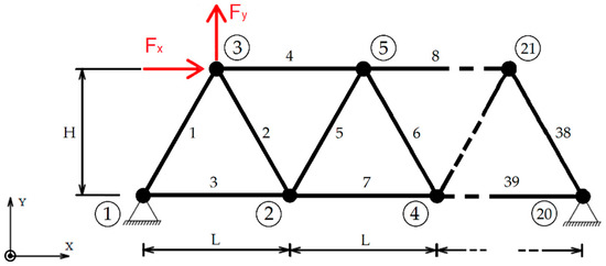
Figure 19. Example 3. Schematic of the truss system structure subjected to the force vector F_load at Node_3, comprising 39 bars and 21 nodes.

The system is essentially composed of a prototype subsystem that generally includes bars modeled as Euler–Bernoulli beams and joint nodes labeled 1, 2, 3, and 4. The last node has no further continuation, as it represents the end of the structure.

The force F_{load m} serves as a verification check of the computed force F_load. The force F_{load m} is derived from the forces within the system, specifically from the equilibrium at Node_3 in Subsystem 1; see Figure 20.

$$\sum F_x=0; F_{\mathrm{l}\mathrm{o}\mathrm{a}\mathrm{d} x}+N_4-{\displaystyle \frac{N_1}{2}}+{\displaystyle \frac{N_2}{2}}=0$$

(51)

$$\sum F_y=0; F_{\mathrm{l}\mathrm{o}\mathrm{a}\mathrm{d} y}-{\displaystyle \frac{\sqrt{3}{·N}_1}{2}}-{\displaystyle \frac{\sqrt{3}{·N}_2}{2}}=0$$

(52)

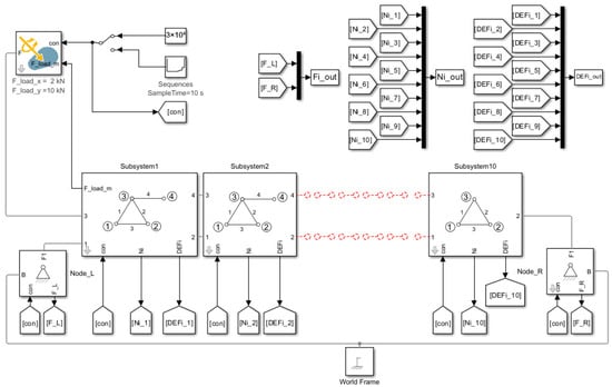
Figure 20. Example 3. Model comprising Euler–Bernoulli beams and joint nodes. Truss system structure subjected to the force vector F_load at Node_3, Subsystem 1. Created in MATLAB–Simscape Multibody based on the schematic in Figure 19.

The force F_load represents the external load acting on the system. In cases where multiple external forces are applied to the system, the maximum force is selected for the control measurement. For clarity, symbolic calculations are no longer included at this stage; instead, the individual results are organized in a table. First, the theoretical calculation is presented, followed by the results obtained from the model.

The model, after optimization, achieved an accuracy consistent with that of the theoretical model up to six decimal places. A visualization of the deformed state was performed for a defined norm of the displacement vector ||δ₃|| = 0.1 m at Node_3. This value is not critical, and is used solely for an exaggerated display of the deformation. See Figure 21.

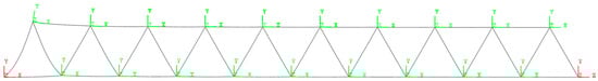
Figure 21. Visualization of the deformed state of the model for Example 3.

In this simulation, the computational time increased; however, the level of accuracy was maintained. The numerical computation conditions for all models in Example 1, Example 2, and Example 3 were identical. The same solver (ode15s) was used, along with consistent settings for the absolute tolerance (10⁻³), relative tolerance (10⁻³), maximum iteration step (0.01), within a variable step.

5. Discussion

During simulations in Simulink and Simscape models, certain differences in computational accuracy arise when the levels of input quantities are varied. These differences can naturally be addressed in “Model Settings–Solver” [19] (pp. 311–319) or the online aid [28] by imposing stricter requirements on parameters such as “Max step size”, “Absolute tolerance”, and “Relative tolerance”, either with respect to zero or relative to previous iterations. For the computations involving the given truss systems, where a static problem was analyzed, the recommended solvers ode15s, ode23s, ode23t, and ode23tb were used for so-called stiff problems. These solvers exhibit significantly higher speed compared to methods designed for nonstiff problems, such as ode45, ode23, or ode113. Another interesting approach that can be taken to further improve computational accuracy involves adjusting the proportionality (scaling) of the input quantity in the system, whether the system under analysis is a static structure, as in our case, or another type of system. Based on this proportionality, it is sufficient to identify a known quantity within the system (in our case, F_load) and redefine it based on the computational outputs (i.e., F_{load m}). For the simplest evaluation of output quantities, we opted for implementing step changes in proportionality using the multiplier constant con within individual sequences. Data representing steady-state values were isolated using a time Lag and Lead to exclude transient responses, which would otherwise distort the output value of F_{load m.} Figure 14, Figure 15 and Figure 16 clearly demonstrate that the accuracy of the computation varies depending on the level of the load force F_load. The optimum is achieved when the mean value of F_{load m} closely matches F_load while maintaining minimal swing. For example, if, for a given sequence k, the mean value of F_{load m} is closer to F_load, but the swing is large enough to extend into the mean calculated in sequence (k−1), then the probability of the calculation being accurate is not 100%. We observed that this proportionality cannot be easily generalized for all systems. It depends on numerous parameters of the system. If parameters such as the diameter of the bars or the Young’s modulus are altered, the optimal setting for the computation also changes. Regarding damping, the coefficients were selected to be the minimum necessary. For bars subjected to Rayleigh damping, the default values of b_m and b_k were retained, as they can essentially be nearly negligible. This is because very small increments of deformation are considered, which are proportionally scaled. In the case of solid bars, the damping coefficient b and the damping of supports b_rj were only increased to the level necessary to suppress undesirable transient responses during the computation.

The examples are divided into models that differ in their types of nodes and bars. The aim was to assess their influence on static analysis and the visualization of deformation. The models constructed from Euler–Bernoulli beams or from solid bars with one degree of freedom (1 DOF) and joints delivered the best results when compared with the theoretical model, as shown in Table 1, Table 2 and Table 3. However, it should be noted that models with solid bars and one DOF are generally unsuitable for dynamic simulations due to the non-uniform distribution of mass elements along the length of the bar. Models using locked joints may, in some cases (such as welded joints), reflect physical reality, but they show lower agreement with the theoretical model. This discrepancy arises because the direction of internal forces in the bars changes during deformation, a behavior that conventional joints can accommodate. For visualizing deformation, physical structures composed of copper elements were deliberately created due to copper’s excellent ductility (see Figure 17d and Figure 18d). These structures were deformed between two holding plates to prevent undesired buckling along the z–axis. Models 1.3 and 2.3 (see Figure 17c and Figure 18c) exhibited the fastest computations and provided a good approximation of the deformed shape. The time required for the calculation depends on the number of system elements. See Figure 22.

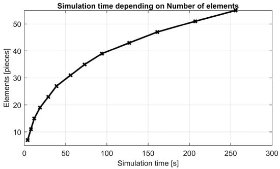
Figure 22. The calculation depends on the number of system elements.

Models 1.1 and 2.1 (Figure 17a and Figure 18a) also achieved accurate shape approximations when higher levels of Rayleigh damping were applied to the bars, albeit at the cost of significantly longer computational times. The final extended model depicted in Figure 19 was developed specifically to test the precision and computational speed for more complex structures.

6. Conclusions

This article provides a comprehensive explanation of a fundamentally simple approach to enhancing computational accuracy within the Simulink environment. It builds on previous work and explores the potential of utilizing built-in tools available as part of the software package employed in our research. Our interest lay in assessing the results in terms of accuracy and determining the extent to which the simulations in Simulink deviated from theoretical calculations. Although this may represent an extreme requirement in terms of precision, its scaling offers a viable means of improving computational accuracy.

As discussed in Section 5, the examples are categorized into models differing in their types of nodes and bars. The aim was to investigate their influence on computational accuracy and deformation visualization in order to identify the optimal model in terms of theoretical calculations and, where applicable, visualization. From a computational standpoint, the model composed of Euler–Bernoulli beams and joints proved to be the most suitable, and it is also appropriate for dynamic simulations. However, regarding the visualization of extreme deformations, the results were not as clear-cut as in the case of computational analyses. It is therefore not possible to definitively identify a single model as the most suitable in this context. It should also be noted that the physical structures themselves were not perfect either, considering aspects such as the precision of node placement within the system, their mechanical implementation, structural strength, material quality, and similar factors. Additionally, the ratio of the length of the bar to its cross-section played a significant role in the collapse behavior of the physical truss structure. Two physical structures were experimentally constructed, each using bars of different diameters. Under the specified dimensions, working with a smaller cross-section proved more advantageous during loading. For more complex structures, the required computational time increased even though the desired level of accuracy was maintained.

References

- Ondocko, S.; Svetlik, J.; Jánoš, R.; Semjon, J.; Dovica, M. Calculation of Trusses System in MATLAB—Multibody. Appl. Sci. 2024, 14, 9547. [Google Scholar] [CrossRef]
- MathWorks, Inc. Simscape™ Multibody™ Getting Started Guide. The MathWorks. 2025. Available online: https://www.mathworks.com/help/pdf_doc/sm/sm_gs.pdf (accessed on 17 June 2025).
- MathWorks, Inc. Simscape™ Multibody™ User’s Guide. The MathWorks. 2025. Available online: https://www.mathworks.com/help/pdf_doc/sm/sm_ug.pdf (accessed on 17 June 2025).
- Langtangen, H.P.; Pedersen, G.P. Scaling of Differential Equations; Springer Nature: Berlin/Heidelberg, Germany, 2016. [Google Scholar]
- Bradley, D. What is mechatronics and why teach it? Int. J. Electr. Eng. Educ. 2004, 41, 275–291. [Google Scholar] [CrossRef]
- Bishop, R.H. Mechatronics: An Introduction; CRC Press: Boca Raton, FL, USA, 2017. [Google Scholar]
- MathWorks, Inc. SimMechanics™ 3 User’s Guide; The MathWorks: Natick, MA, USA, 2009. [Google Scholar]
- Hroncova, D.; Pastor, M. Mechanical system and SimMechanics simulation. Am. J. Mech. Eng. 2013, 1, 251–255. [Google Scholar]
- Frankovský, P.; Hroncová, D.; Delyová, I.; Virgala, I. Modeling of dynamic systems in simulation environment MATLAB/Simulink–SimMechanics. Am. J. Mech. Eng. 2013, 1, 282–288. [Google Scholar]
- MathWorks, Inc. System Scaling by Nominal Values. 2025. Available online: https://www.mathworks.com/help/releases/R2025b/simscape/ug/system-scaling-by-nominal-values.html?searchHighlight=command+scaling&s_tid=doc_srchtitle#mw_3cc30ae6-fec4-4118-a0d3-032dbf0901cc (accessed on 3 October 2025).
- Miller, S.; Soares, T.; Weddingen, Y.V.; Wendlandt, J. Modeling flexible bodies with simscape multibody software. In An Overview of Two Methods for Capturing the Effects of Small Elastic Deformations; MathWorks: Natick, MA, USA, 2017. [Google Scholar]
- Bauchau, O.A.; Craig, J.I. Euler–Bernoulli beam theory. In Structural Analysis; Springer: Dordrecht, The Netherlands, 2009; pp. 173–221. [Google Scholar]
- Trebuňa, F.; Šimčák, F. Odolnosť Prvkov Mechanických Sústav; Technická Univerzita: Košice, Slovakia, 2004. [Google Scholar]
- Lengvarský, P.; Pástor, M.; Bocko, J. Riveted Joints and Linear Buckling in the Steel Load–bearing Structure. Am. J. Mech. Eng. 2017, 5, 329–333. [Google Scholar]
- Karnovsky, I.A.; Lebed, O. Advanced Methods of Structural Analysis; Springer Nature: Berlin/Heidelberg, Germany, 2021. [Google Scholar]
- Plevris, V.; Ahmad, A. Deriving analytical solutions using symbolic matrix structural analysis for continuous beams. Sci. Rep. 2025, 15, 1–16. [Google Scholar] [CrossRef] [PubMed]
- Florian, Z.; Pellant, K.; Suchánek, M. Technická mechanika I–Statika; Vysoké Učení Technické v Brně: Brno, Czech Republic, 2004. [Google Scholar]
- Available online: https://github.com/stefanondocko/AddOptimInSimulink (accessed on 17 June 2025).
- MathWorks, Inc. Using Simulink. In Simulink–Model–Based and System–Based Design; MathWorks Inc.: Natick, MA, USA, 2002. [Google Scholar]
- MathWorks, Inc. Speed Up Simulation. 2023. Available online: https://www.mathworks.com/help//releases/R2021a/simulink/ug/speed-up-simulation.html (accessed on 22 June 2025).
- Gavin, H.P. Classical Damping, Non–Classical Damping and Complex Modes; Duke University: Durham, NC, USA, 2018. [Google Scholar]
- MathWorks, Inc. Choose an ODE Solver. Ordinary Differential Equations. 2025. Available online: https://uk.mathworks.com/help/matlab/math/choose-an-ode-solver.html (accessed on 17 June 2025).
- Oršanský, P.; Ftorek, B. Štatistické a Numerické Metódy; EDIS–ŽU: Žilina, Slovakia, 2017. [Google Scholar]
- Buša, J.; Pirč, V.; Schrotter, Š. Numerické Metódy, Pravdepodobnosť a Matematická Štatistika; FEI TU: Košice, Slovakia, 2006. [Google Scholar]
- Available online: https://github.com/vplevris/SymbolicMSA-2DTrusses (accessed on 17 June 2025).
- Murín, J.; Hrabovský, J.; Kutiš, V. Metóda Konečných Prvkov—Vybrané Kapitoly pre Mechatronikov; Slovenská technická univerzita v Bratislave: Bratislava, Slovakia, 2014. [Google Scholar]
- Öchsner, A. Euler–Bernoulli beam theory. In Classical Beam Theories of Structural Mechanics; Springer: Berlin/Heidelberg, Germany, 2021; pp. 7–66. [Google Scholar]
- MathWorks, Inc. Solver–Solver that Computes States and Outputs for Simulation. 2025. Available online: https://uk.mathworks.com/help/simulink/gui/solver.html (accessed on 17 June 2025).
Disclaimer/Publisher’s Note: The statements, opinions and data contained in all publications are solely those of the individual author(s) and contributor(s) and not of MDPI and/or the editor(s). MDPI and/or the editor(s) disclaim responsibility for any injury to people or property resulting from any ideas, methods, instructions or products referred to in the content. |
© 2025 by the authors. Licensee MDPI, Basel, Switzerland. This article is an open access article distributed under the terms and conditions of the Creative Commons Attribution (CC BY) license (https://creativecommons.org/licenses/by/4.0/).