Abstract
Off-system bridges are critical components of the United States’ transportation infrastructure, providing essential access to rural communities and enabling residents to reach vital services such as employment, education, and healthcare. Many of these bridges are structurally deficient, functionally obsolete, and unmaintained. This disproportionately hinders the mobility of underserved populations, worsening socioeconomic disparities. Despite existing research, there is insufficient focus on the unique challenges posed by off-system bridges, including handling the class imbalanced nature of the bridge condition rating dataset. This paper predicts bridge deck conditions by using Generative Adversarial Networks with Focal Loss (GAN-FL) to generate synthetic data which enhances precision–recall balance in imbalanced datasets. Results show that integrating GAN-FL with random forest (RF) classifiers significantly enhances the performance of minority classes, improving their precision, recall, and F1 scores. The study finds that augmenting training data using GAN-FL greatly enhances minority class prediction, thereby assisting in accurate bridge condition modeling.
1. Introduction
Nearly half of the 587,000 bridges on public highways in the United States that are longer than 6.1 m (20 feet) are classified as off-system bridges, meaning they are not covered by the Federal Aid System. Due to a lack of resources for monitoring and maintenance, these structures which are mostly found on local roads and rural collectors frequently experience extreme neglect and decay [1]. Approximately 30% of off-system bridges are either structurally flawed or no longer functioning. These bridges connect remote settlements to low-volume roads, giving locals access to jobs, healthcare, and educational opportunities [2]. Closing these bridges will thereby aggravate socioeconomic gaps by disproportionately affecting the mobility of marginalized populations [3]. States are required to assess their off-system bridge needs and set aside at least 15% of their Bridge Formula Program funding expressly for these bridges under the bipartisan infrastructure law (BIL), which is administered by the federal highway administration (FHWA) [4,5]. To guarantee that their structural conditions are properly maintained, local administrations must thus identify and rank their off-system bridges.
Engineers and inspectors must give off-system bridges top priority for evaluation and maintenance due to the large number of defective bridges [6]. Regretfully, the evaluation of off-system bridges is usually ignored in current research, which ignores their circumstances and difficulties [6]. Quadri [7] found that Truck ADT data was available for 99.4% of on-system inspections in the national bridge inventory (NBI), with the remaining 0.6% estimated based on the bridge’s functional classification. In contrast, only about 70% of off-system inspections had Truck ADT data available, and the remaining 30% could not be accurately estimated using other variables. This issue can be partly attributed to discrepancies and inefficiencies in data collection practices between local, state, and federal levels.
These bridges are complicated to plan and manage, requiring careful consideration of several variables, such as lifetime, operating context, environmental conditions, and the possible effects of required closures. However, to guarantee off-system bridges’ structural integrity and meet transportation fairness objectives, maintenance must be prioritized. Advanced degradation models have a lot of promise, even though many inspectors still use traditional procedures like visual inspections, chain drag methods, and hammer sounds to evaluate bridge conditions. Bridge maintenance has a bright future thanks to these models, which can improve forecasts of bridge conditions and direct wise repair choices [8].
The main source of data for bridge degradation modeling in the US is the NBI, which was created by the FHWA in 1972 [9,10]. To distinguish between on-system and off-system bridges, it offers information on bridge ownership [11]. Every two years, bridges included in the NBI are required to undergo regular inspections in addition to the national bridge inspection standards (NBIS). During these inspections, important components, including decks, superstructures, and substructures, have their condition ratings (Table 1) documented. Table 1 summarizes the federal highway administration’s (FHWA) standard condition rating codes used to assess the structural integrity and serviceability of bridge components. A single-digit rating system with a range of 0 to 9 is used to evaluate these circumstances and determine the general health of the component under inspection. To assist engineers and administrators in making decisions, the NBI coding guide [11] also documents other characteristics that are crucial for modeling bridge deterioration.

Table 1.
Condition rating codes as described in NBI. Reprinted/adapted with permission from Ref. [11]. Copyright 2025, Federal Highway Administration (FHWA).
Condition ratings have been utilized by earlier studies to simulate the degradation of bridge components, which has made it easier for BMS to direct maintenance, rehabilitation, and replacement decisions. The three primary types of these models are artificial intelligence (AI), probabilistic, and deterministic [12,13,14]. Deterministic models establish fixed correlations between independent variables including age, average daily traffic, and environmental conditions and the deterioration of bridges [15,16]. They utilize exponential/logistic equations or polynomials as mathematical representations to explain these interactions [17,18]. Iterative modeling is frequently necessary to find the best-fitting models and essential variables, which can be time-consuming. The degradation of bridge conditions, on the other hand, is seen as a stochastic process by probabilistic models, which take measurement errors and uncertainties from unknown factors into account [19]. Deterioration’s intrinsic unpredictable nature is well captured by Markovian techniques [10,20].
Similarly, artificial intelligence models have the potential to transform our comprehension of bridge degradation [21,22,23,24,25]. By identifying trends in training datasets, these models can make accurate predictions and revolutionize bridge infrastructure [9] For example, Chencho et al. [21] evaluated structural damage using a RF regressor and discovered a direct correlation between higher damage severity and a decrease in stiffness parameters [21]. Fernandez-Navamuel et al. [22] used Deep Learning Enhanced Principal Component Analysis in a similar manner to track structural irregularities in bridges. According to [23], they discovered that the model’s ability to identify outliers in bridge situations was greatly enhanced by the addition of residual connections. Rajkumar et al. [8] developed an autoencoder-random forest model to forecast bridge condition ratings using the NBI dataset for Florida.
Recent studies further demonstrate that data-driven and hybrid learning frameworks combining decision trees, neural networks, and feature selection algorithms can substantially enhance the interpretability and accuracy of deterioration forecasting across diverse bridge types [26,27,28,29,30,31,32,33,34,35,36,37,38,39]. In particular, ensemble and deep learning approaches have been shown to capture nonlinear degradation patterns and improve class-level prediction under highly imbalanced datasets, enabling more reliable prioritization of maintenance interventions [40,41,42,43,44,45,46,47,48,49]. Moreover, advanced augmentation techniques and generative models are increasingly applied to structural health monitoring, mitigating data scarcity and boosting detection sensitivity for minority or rare condition states [50,51,52,53,54,55,56,57].
However, stakeholders looking for precise insights for management and maintenance choices face difficulties when dealing with unbalanced data. This emphasizes the necessity of machine learning techniques for bridge prediction models that improve classification accuracy through appropriate handling of class imbalances. If these gaps are not filled, model accuracy across hard to classify classes will be reduced, which could result in incorrect maintenance priorities and increased risks of infrastructure failure. Accordingly, this study uses Texas Department of Transportation (TxDOT) data to create interpretable machine learning models that forecast bridge deck condition ratings and successfully alleviate class imbalances [26]. The dataset, derived from the historical NBI database for Texas, covers the period from 1900 to 2024. This dataset provides detailed information on bridge structures, including deck condition ratings and associated structural attributes, allowing for a comprehensive analysis of bridge condition over time. A total of 1443 bridges (obtained by removing on system bridges from the NBI dataset) were included in the analysis, encompassing a variety of bridge types and condition classes, ensuring comparability across samples. These data are comparable across bridges, as the NBI is a nationwide dataset developed and maintained by the Federal Highway Administration (FHWA) with standardized reporting formats, uniform definitions of bridge attributes, and consistent rating procedures for bridge conditions [9]. This ensures that bridges of different types, locations, and ages can be meaningfully compared, making the dataset suitable for developing and evaluating machine learning models for multiclass bridge condition classification [58]. The data were preprocessed to standardize features and remove inconsistencies, enabling a robust input for model training and evaluation.
2. Methodology
Bridge condition classification presents unique challenges that standard machine learning approaches struggle to address. Data collected from structures is often limited and unevenly distributed, with certain conditions being overrepresented while others, though critical, are underrepresented [55,56]. Standard classifiers, such as RF or SVM, can achieve reasonable overall accuracy; however, they often struggle to correctly identify underrepresented or borderline conditions and are prone to misclassifying bridges with subtle differences in condition features [55]. Deep learning approaches, such as convolutional neural networks (CNNs), can automatically learn relevant features and have been successfully applied to concrete surface damage classification. Nevertheless, these methods also typically require extensive labeled datasets and are often not generalized enough to handle multiclass bridge condition classification, particularly when classes are closely related or data is imbalanced [56]. In addition, subtle differences between adjacent bridge conditions can be difficult to capture, leading to systematic misclassifications that can undermine decision-making in structural health monitoring [57]. Relying solely on these conventional classifiers would risk overlooking critical distinctions necessary for accurate bridge monitoring and decision-making [55,56,57,58,59,60].
To overcome these issues, the proposed framework integrates generative adversarial networks (GAN)-based data augmentation, focal loss, and RF. GAN augmentation expands the training set by generating realistic synthetic examples for challenging conditions, improving the model’s ability to learn the statistical patterns that define each class.
In addition, focal loss is incorporated to prioritize harder-to-classify samples by down-weighting the contribution of well-classified instances during training. This ensures that the model focuses on minimizing misclassification between adjacent or confusable bridge conditions, improving class-specific performance. Finally, RF serves as a robust and interpretable classifier, benefiting from ensemble learning to generalize well across all classes. By integrating these components, the proposed framework leverages the strengths of each method to handle class imbalance, capture subtle distinctions between conditions, and achieve measurable improvements in class-wise performance, as reflected in F1-scores and the confusion matrix.
The training dataset is supplemented with synthetic data using a GAN trained with focal loss, which greatly enhances the representation of minority classes. Precision-recall curves, confusion matrices, and F1-scores are used to assess the performance of different models.
Unlike traditional oversampling methods such as SMOTE, which rely on linear interpolation and often distort the underlying data distribution [30], our approach leverages a GAN-based framework to learn the nonlinear minority class distribution directly. While recent studies have used GANs to generate synthetic data for class imbalance problems [61,62], most of these approaches rely solely on adversarial training for data augmentation. By contrast, we integrate Focal Loss into the discriminator, enabling the model to prioritize hard-to-classify minority samples [63], thereby improving convergence and diagnostic accuracy under imbalance. Furthermore, whereas prior structural health monitoring studies have primarily utilized CNN-based classifiers trained on augmented data [63], we introduce a RF ensemble after GAN-FL training. This hybrid design reduces model variance, improves generalization on small-sample datasets, and enhances interpretability for multiclass bridge condition assessment. To our knowledge, this GAN-FL + RF framework (architecture presented in Figure 1) has not been applied to structural health monitoring, marking a distinct methodological contribution of our work to literature.
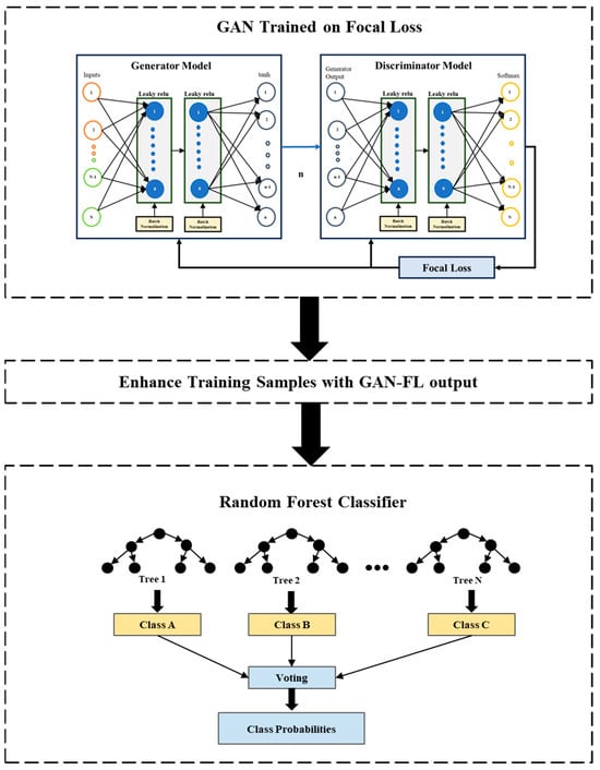
Figure 1.
Model Architecture.
2.1. Feature Selection and Regularization
Data collection was followed by several preprocessing steps, which included data cleaning, removing irrelevant entries, and normalization, for ensuring its usability for modeling purposes. Normalization was performed using Standard Scalar function. Then, the training, testing, and validation sets were split with a 60-20-20 ratio. Thereafter, the Boruta algorithm was employed to select the best features to be retained for analysis. This enhanced algorithm is based on the RFt method that iteratively identifies the truly important variables by comparing the importance of original attributes with their randomized counterparts. This approach helps in refining the selection of relevant features in high-dimensional classification tasks [27,28]. The specific variables selected include the year the structure was built (Year Built), bridge improvement costs (Bridge Improv Cost), structural evaluation ratings (Struct Eval), deck geometry (Deck Goem), gross loading ratings (Gross Loading), substructure condition ratings (Substruc Cond), superstructure condition ratings (Superstruc Cond), deck type, length of maximum span (Max Span Length), deck width, structure length (Struc Length), Annual Daily Truck Traffic (Truck ADT), and Annual Daily Traffic (ADT), as reported in Figure 2. Ridge regression (L2), which added a penalty equal to the square of the magnitude of coefficients to help prevent overfitting, was combined with TomekLinks, which eliminates pairs of instances that are close to one another but belong to different classes [29], to address class imbalance in the original data to a certain level.
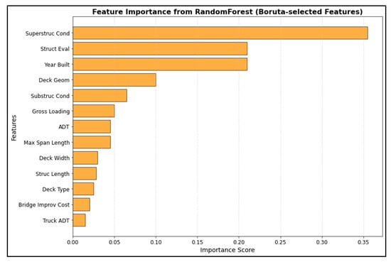
Figure 2.
Feature Importance Values.
2.2. Generative Adversarial Network (GAN) with Focal Loss (FL)
Class imbalance [57,58,59,60] can be effectively mitigated by expanding the training dataset using sampling-based techniques. Chawla et al. [30] introduced the widely adopted synthetic minority oversampling technique (SMOTE), which generates synthetic samples through random linear interpolation between a minority sample and its K-nearest neighbors. Over time, SMOTE has evolved into numerous advanced variants and remains a popular choice for handling class imbalance. However, such methods often modify the original data distribution and are limited by insufficient feature representation. In contrast, GANs and RF classifiers leverage their ability to learn complex, non-linear data patterns, producing diverse and realistic samples. Unlike SMOTE’s linear interpolation approach, GANs capture intricate data structures, making them particularly effective for addressing imbalanced datasets with high-fidelity sample generation [31,32].
Research has shown that integrating focal loss (FL) into neural networks designed for classification significantly improves their diagnostic efficiency, particularly for minority samples [33]. For example, Li et al. [34] demonstrated that integrating FL into neural networks significantly improved fault diagnosis performance under imbalanced conditions. Their proposed method, VGAIC-FDM, combined variational autoencoder generation adversarial networks with an improved convolutional neural network to balance the dataset and enhance diagnostic efficiency. The approach utilized continuous wavelet transform to capture local features of vibration signals, followed by dimensionality reduction through grayscale conversion of wavelet time-frequency images. This was complemented by sample augmentation via the adversarial network and training with a Focal Loss-optimized CNN classifier, resulting in improved accuracy and F1-score values in fault diagnosis.
Building on the advantages of combining GAN and FL to address class imbalances more effectively than traditional methods like SMOTE, this study utilizes the GAN-FL model to manage unbalanced datasets and enhance structural health monitoring of bridges.
Two neural networks, the discriminator, and the generator, are combined in a competitive framework to create the GAN, which separates generated and actual data [35]. Through feedback from the discriminator, the generator gains knowledge and modifies its parameters to provide more realistic results. The generator aims to trick the discriminator while the discriminator improves its capacity to recognize phony data [36].
Random noise is usually the generator’s initial input, which it then converts into synthetic data samples via several layers. It models the data’s complexity using activation functions [37]. Convolutional or fully connected layers are used by the discriminator, which is frequently designed to resemble a typical classification network, to determine if the input data is produced or real [38]. Loss functions are used to optimize both networks to stabilize training and minimize problems such as mode collapse. This model’s ability to produce synthetic data for underrepresented classes, hence addressing class imbalance in datasets, is a significant benefit in enhancing minority class performance [39]. To balance the training data, the generator can create synthetic examples after learning the minority class distribution [40]. For imbalanced classification issues, this can enhance model performance for the minority class, resulting in improved generalization and more precise predictions.
The generator model for this work is constructed using a sequential architecture with two hidden layers, each of which is followed by LeakyReLU activation functions (Equation (1)) and batch normalization [41]. The fading ReLU issue is lessened by this activation function, which permits a slight, non-zero gradient while the unit is not active (α = 0.01).
A tanh activation function (Equation (2)) is used in the generator’s last layer to guarantee that the output corresponds to the appropriate number of features. The tanh activation function facilitates zero-centered data and enhances convergence during training by introducing non-linearity, particularly in buried layers of neural networks.
Additionally, a sequential architecture with two hidden layers each followed by batch normalization and LeakyReLU activation functions is used to construct the discriminator model.
A softmax activation function (Equation (3)) is used in the discriminator’s last layer) (where represents the number of classes and is the weight vector for class ). To match the number of classes in the classification problem, this function will assist in producing probabilities for each class [42].
The Focal Loss function and the Adam optimizer [43] with the set learning rate are used to create the discriminator and generator. The generator and discriminator are then combined to create the GAN model. To guarantee that only the generator is modified during the GAN training phase, the discriminator is made to be non trainable. The Focal Loss function (Equation (4)) and the Adam optimizer with the given learning rate are then used to compile the GAN.
where represents the predicted probability of the model for the true class, represents a scaling factor, and adjusts the focusing parameter to reduce the weight of easy examples.
The GAN model is constructed by combining the generator and the discriminator into a unified architecture. During the training process, the discriminator is set to non-trainable, ensuring that the optimization is solely focused on updating the weights of the generator. A gamma value of 0.2 and an alpha value of 0.25 are set for the loss. Furthermore, since the problem is a multi-class classification problem, the focus loss is tracked using the categorical cross-entropy function. Equation (5) specifies the Generator Loss, which measures how effectively the generator can produce realistic data while Equation (6) outlines the Discriminator Loss, which quantifies the discriminator’s ability to distinguish between real and generated data. Finally, Equation (7) represents the combined GAN objective trained using Adam Optimizer, incorporating both the generator and discriminator losses, and the performance is assessed through Focal Loss to refine the model’s ability to generate high-quality data.
where and represent the loss function for the generator and discriminator, respectively. refers to the expectation over the real data , drawn from the true data distribution . Here, is the discriminator’s estimated probability that the real data is authentic, and the term applies the Focal Loss to the discriminator’s prediction for real data. Similarly, represents the expectation over the random noise , which is used as input to the generator. The term indicates the probability that the generated data is fake, which is utilized to compute the Focal Loss for the generated data. Finally, ) applies Focal Loss to the discriminator’s prediction for the generated data. The notation represents the min–max optimization approach, where the generator aims to minimize its loss, while the discriminator seeks to maximize its own loss.
The number of hidden units in the discriminator and generator, the learning rate, and the input dimensions are the hyperparameters used to fine tune the GAN-FL model [45] utilizing Randomized Search CV [45]. The selected hyperparameters are commonly reported in foundational and applied GAN studies [39,40,41,42,43,44]. With a patience value of 40 epochs, early halting is used to avoid overfitting [45].
Using the generator to create synthetic data, the discriminator is trained to differentiate between authentic and fraudulent data. The GAN is then used to train the generator to generate data that is more realistic. The discriminator and generator losses are tracked, and the optimal combination of hyperparameters is chosen based on the lowest total loss. The best and tested hyperparameters are shown in Table 2. Focal Loss, which is intended to rectify class imbalance by concentrating more on difficult-to-classify samples, is used to monitor the GAN.
Table 2.
Tested and Optimized Hyperparameters.
2.3. Random Forest (RF) Classifier
The RF Classifier is a powerful ensemble learning method used in this study. The decision to employ a RF classifier stems from its balance between predictive performance and practical applicability. Compared to boosting algorithms, which may risk overfitting by sequentially refining weak learners, RFs use an ensemble of independently trained trees, thereby enhancing model stability and minimizing variance. Furthermore, in contrast to Artificial Neural Networks (ANNs), which typically demand extensive datasets and a high number of features to achieve optimal performance, RFs are well-suited for contexts with limited data availability or fewer predictor variables. This makes them a more appropriate and efficient choice for the scale and nature of the data used in this study. As mentioned previously, it has been shown that integrating Focal Loss (FL) into neural networks designed for classification significantly improves their diagnostic efficiency, particularly for minority samples [33].
Based upon this logic, we feed the GAN-FL output into the RF classifier for predicting multiclass probabilities. The classifier consists of decision trees, with each tree contributing to the prediction of class probabilities for each instance in the dataset . For each instance , each of the trees make a prediction in the form of a probability distribution over the possible classes. The predicted probability (Equation (8)) for class is calculated by averaging the predicted probabilities across all trees in the forest, as shown in Equation (8).
where is the predicted probability of instance belongs to class while is the predicted probability of class for instance from the tree. In this way, the RF Classifier is trained using the training dataset and the synthetic data produced by the GAN-FL model. The additional training data from GAN-FL helps the RF classifier perform exceptionally well on classification tasks, outperforming its actual potential, especially when dealing with large dimensionality and unbalanced datasets [47], thereby enhancing the predictive capabilities of this ensemble model.
To guarantee reproducibility, the classifier in this study is started with a fixed random seed, and a thorough parameter grid is established for hyperparameter optimization. The number of estimators, which determines the number of trees in the forest [48]; the maximum number of features taken into consideration for splitting at each node [49]; the maximum depth of each tree; the reduced number of samples needed to split an internal node; and the fewer samples needed to be at a leaf node [50] are among the optimized hyperparameters.
Table 2 displays the tested and optimal set of hyperparameters. For both GAN and RF models, RandomizedSearchCV is used to maximize model performance, enabling effective parameter space exploration by random sampling across these specified hyperparameters [51]. These hyperparameters and their ranges were selected as they were exhaustively used in previous studies [47,48,49,50,51]. By dividing the dataset into five subgroups and using 5-fold cross-validation, this method makes sure that the model is validated on each subset while being trained on the remaining data [64]. This technique helps prevent overfitting and improves the accuracy of performance estimations [52].
2.4. Accuracy and Interpretation
While previous studies often report overall accuracy, precision, recall, or F1-score, these metrics alone are insufficient for imbalanced datasets and do not capture performance at the class level. In contrast, this study frames bridge condition assessment explicitly as a multiclass classification problem [55,56,57], calculating precision, recall, and F1-score for each condition. This ensures that the evaluation reflects the model’s ability to correctly identify each class, including underrepresented or closely related conditions, rather than being dominated by the most frequent classes. The confusion matrix and F1 score comparisons (pre- and post-GAN-FL treatment) further complements this evaluation, providing detailed insights into misclassifications and the balance between precision and recall across all classes [53,54]. This thorough evaluation framework makes it possible to conduct a thorough analysis of the RF Classifier’s performance, guaranteeing that the model achieves high accuracy and successfully handles class imbalances.
3. Results and Discussions
The study’s findings and analysis are presented in this section, with an emphasis on how well the suggested approaches alleviate class disparities and enhance the model’s precision and interpretability. Figure 3, which displays the distribution of the frequency of occurrence for all conditions, is provided to give some preliminary insights into the nature of the data. All experiments were conducted using Python 3.12.4 (Anaconda, 64-bit, MSC v.1929).
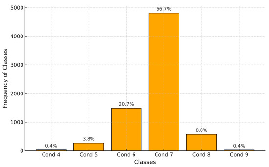
Figure 3.
Distribution of Frequency of Occurrence for all conditions.
It is evident from Figure 3 that the dataset is unbalanced. To comprehend the initial model results, a RF classifier was trained using a combination of Ridge regularization and TomekLinks, as well as Boruta-selected features. It is important to note that all x Together, these techniques made sure that the dataset was balanced and that the model was resistant to overfitting, which enhanced the analysis’s overall effectiveness and dependability. The results of the first RF classifier are shown in Table 3.
Table 3.
Initial RF Classification Results.
The model’s accuracy and resilience under varied circumstances are thoroughly assessed by its performance indicators, which include precision, recall, F1-score, and support. Table 3 demonstrates that the original RF model has significant errors in precision and recall for Conditions 4, 5, and 8, even with regularization efforts to rectify class imbalances. With F1-scores of 0, 0.09, and 0.02 for these scenarios, respectively, the model performs poorly, underscoring the difficulties caused by the dataset’s imbalance. With a precision, recall, and F1-score of zero, Condition 4 displays no accurate predictions, suggesting that the model was unable to accurately identify any instances across the eight data. This implies that the condition is extremely complex or that the model might not have enough training data. Condition 5′s F1-score is 0.09 due to its poor precision of 0.22 and even poorer recall of 0.05. This shows that there are substantial challenges in managing this condition across 38 samples, since the model not only fails to detect many real positives but also makes many false positive predictions. Based on 105 samples, Condition 8 performs similarly poorly, with a precision of 0.25, recall of 0.01 and a F1-score of 0.02.
However, based on 308 samples, Condition 6 performs better, with a F1-score of 0.61, precision of 0.68, and recall of 0.56. With a high precision of 0.79, recall of 0.94, and F1-score of 0.86, Condition 7 is the most effective, showing good performance across 977 samples. With a balanced precision, recall, and F1-score of 0.71, condition 9 may not be indicative of larger patterns because it is based on a tiny sample size of 7. The model’s overall accuracy across 1443 samples is 0.76. The precision, recall, and F1-score of the macro average, which assigns equal weight to each condition, are 0.44, 0.38, and 0.38, respectively. With the number of samples in each condition considered, the weighted average displays a F1-score of 0.72, a precision of 0.71, and a recall of 0.76. These averages imply that although the model does well in some circumstances, its subpar performance in others has a major impact on its overall performance.
GAN-FL Enhanced Random Forest Classification (RFC-GAN-FL)
Table 4 shows the generator architecture, which begins with a dense layer with 16,416 parameters and 32 features. A batch normalization layer with 128 parameters comes next. After that, a Leaky ReLU activation layer which lacks trainable parameters is used. Usually, the slope of the function’s negative portion is a fixed hyperparameter, frequently set to a little value like 0.01. A second batch normalization layer with 128 parameters, another Leaky ReLU activation layer, and another dense layer with 1056 parameters repeat this sequence. The last dense layer in the architecture contains 495 parameters and produces 15 features.
Table 4.
GAN architecture.
Similarly, the discriminator design, which is likewise shown in Table 4, starts with a dense layer of 448 parameters and 32 features. A batch normalization layer with 128 parameters comes next. After that, a Leaky ReLU activation layer which lacks trainable parameters is used. A second batch normalization layer with 128 parameters, another dense layer with 1056 parameters, and another Leaky ReLU activation layer without trainable parameters follow this pattern. The last dense layer of the architecture has 198 parameters and produces 6 classes.
It is important to emphasize that aggregate metrics such as overall accuracy or weighted F1-score can obscure uneven performance across classes, particularly when class distributions are imbalanced. In the context of bridge condition classification, misclassification of minority or critical conditions can have important practical implications. Although the weighted F1-score increased modestly from 0.72 to 0.76 after the intervention, aggregate improvements alone do not fully capture class-level performance. This underscores why the problem identified in this study is evaluated using a multiclass classification task rather than relying solely on overall metrics.
That being said, the performance of minority classes was greatly improved by integrating the GAN with FL (GAN-FL) into the RFC (RFC-GAN-FL), as shown in Table 5. The F1-score improved from 0.09 to 0.34, memory ratings improved from 0.05 to 0.24, and precision scores climbed from 0.22 to 0.60 for Condition 5. The F1-score improved from 0.02 to 0.30, memory scores improved from 0.01 to 0.19, and precision scores improved from 0.25 to 0.74 for Condition 8. These enhancements demonstrate how well the GAN-FL addresses class imbalance and improves the model’s capacity to handle challenging-to-classify cases. However, considering the small number of support samples available for classification, Condition 4 also did not become better. On the other hand, the primary classes’ performances were consistent with the original RF classification performance. This consistency shows that the model’s capacity to correctly categorize the majority classes was unaffected by the GAN-FL integration. Furthermore, every accuracy indicator showed a discernible improvement. Both the weighted average accuracy and the macro average accuracy improved from 0.38 to 0.48 and 0.72 to 0.76, respectively. Additionally, overall accuracy increased from 0.76 to 0.78, indicating the RFC-GAN-FL combination’s greater performance over the RFC alone. These improvements are clearly highlighted in Figure 4.
Table 5.
RFC-GAN-FL classification results.
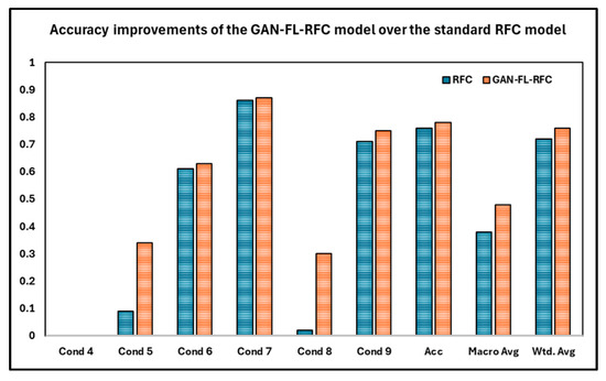
Figure 4.
Accuracy improvements of the GAN-FL-RFC over the standard RFC model.
The model’s performance under various settings is shown in detail in the confusion matrix shown in Figure 5. All the model’s predictions were wrong for Condition 4, and it was unable to accurately identify any instances. The algorithm detected nine cases of Condition 5 accurately, but incorrectly classified 23 instances as Condition 6 and six instances as Condition 7. The algorithm accurately detected 183 instances of Condition 6, but incorrectly classified 5 of these as Condition 5, 119 as Condition 7, and 1 as Condition 9. The model identified 911 instances of Condition 7 accurately, but incorrectly classified 58 instances as Condition 6, 7 instances as Condition 8, and 1 instance as Condition 9. The model detected 20 cases of Condition 8 accurately, but incorrectly classified 84 instances as Condition 7 and one occasion as Condition 9. Six cases of Condition 9 were accurately detected by the model; however, one incident was incorrectly classified as Condition 7. The model works well for Condition 7 overall, but it has trouble with Conditions 4, and 5. For Condition 8, precision increased from 0.25 to 0.74, recall from 0.01 to 0.19, and F1-score from 0.02 to 0.30. Although some bridges labeled as Condition 7 may appear as “misclassified” in the confusion matrix, these predictions reflect the model correcting earlier errors by assigning bridges to their correct categories consistent with the statistical distributions it has learned for each condition. In support of this, the F1-score for Condition 7 increased slightly from 0.86 to 0.87, while Condition 8 showed a substantial improvement from 0.02 to 0.30, demonstrating that the model is systematically refining its predictions and assigning bridges to their true conditions more accurately. In other words, the model is not mislabeling bridges arbitrarily; rather, it is progressively capturing the underlying distinctions between closely related classes. This highlights the importance of class-wise evaluation, as aggregate metrics alone would not capture these nuanced improvements. This data can also be utilized to pinpoint the model’s weak points and guide future optimization initiatives.
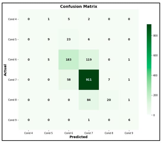
Figure 5.
Confusion Matrix.
With the maximum area under the precision-recall curve (AUC-PR) value of 0.90, as seen in Figure 6, Condition 7 enables the classifier to efficiently detect positive occurrences while reducing false positives and false negatives. Across a range of thresholds, this condition consistently strikes a good balance between high precision and recall. In a similar vein, Condition 9 succeeds admirably with an AUC-PR of 0.83, albeit with somewhat less recall or precision than Condition 7. With an AUC-PR of 0.68, Condition 6 performs quite well, obtaining a respectable balance between recall and precision, although it still lags behind compared to Conditions 7 and 9. Conversely, Conditions 8 and 5 exhibit a large drop in performance, with AUC-PR values of 0.42 and 0.36, respectively, as precision sharply declines as recall rises. With an AUC-PR of just 0.11, Condition 4 performs the worst, showing a limited capacity to correctly anticipate positive occurrences.
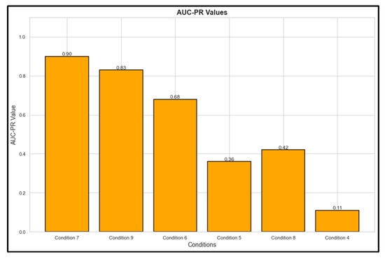
Figure 6.
Area under the Precision–Recall curve.
4. Limitations
The dataset used in this study was obtained from the Texas Department of Transportation and comprised 1443 samples, with only 8 belonging to Condition 4. Due to the extreme class imbalance, GAN–based augmentation was applied to increase representation of this underrepresented category. However, it is important to acknowledge that oversampling methods applied to classes with fewer than 10 original samples may not yield sufficiently robust or generalizable synthetic data unless supported by auxiliary approaches, such as transfer learning. This limitation should be considered when interpreting the results related to Condition 4.
Although this study focuses on developing and validating a technical condition prediction framework for bridges, the analysis did not include a long-term predictive demonstration for an individual bridge. While historical bridge condition data were available, the objective of this study was to evaluate the overall predictive performance of the proposed model rather than to simulate the condition evolution of a specific structure over time (e.g., after 10 or 20 years). Future research will extend this framework to perform longitudinal forecasting for selected bridges, using historical inspection records to generate deterioration trajectories and assess model performance under different maintenance and environmental scenarios. Such an application would further demonstrate the model’s practical value for bridge asset management and maintenance planning.
A key limitation of this study is that the analysis was conducted solely using TxDOT bridge data derived from the National Bridge Inventory. While this provides a rich and standardized dataset, it also constrains the generalizability of the findings, as bridge performance and deterioration patterns can vary across states due to differences in climate, construction practices, traffic loads, and inspection protocols. Future research should therefore evaluate the transferability of the proposed RFC-GAN-FL framework to datasets from other states or regions, encompassing diverse environmental conditions and data collection methodologies. Such validation would further demonstrate the robustness and scalability of the approach for nationwide bridge management applications.
Another limitation of this study is that, while SMOTE is referenced, the work does not provide quantitative comparisons with other oversampling methods such as ADASYN, Borderline-SMOTE, or more recent GAN-based variations. Including such benchmarks could further validate the relative effectiveness of the proposed RFC-GAN-FL framework. Future studies should therefore incorporate systematic comparisons with alternative oversampling and data augmentation strategies to more comprehensively demonstrate the advantages and potential trade-offs of the proposed method.
While the model achieves improved predictive performance, the “black box” nature of machine learning approaches may limit their practical adoption in bridge management and policy contexts, where decision-makers often require transparency regarding which variables most strongly influence outcomes. Future research should incorporate explainable AI techniques such as SHAP or LIME to identify the most influential features driving model predictions. This would not only enhance the interpretability and trustworthiness of the framework but also increase its utility for practitioners and public agencies responsible for infrastructure decision-making. Such steps will inturn facilitate more effective and accountable infrastructure management, helping to prioritize critical maintenance tasks and ensuring the safety and longevity of off-system bridge infrastructure.
Finally, this study has not yet been validated on fully independent datasets beyond the TxDOT data used for model development and evaluation. The absence of such external validation limits the ability to confirm the generalizability and robustness of the proposed framework in other contexts. Future work should prioritize testing the model on independent datasets, ideally from different states or agencies, to strengthen its credibility and enhance trustworthiness for broader deployment in bridge management applications.
5. Conclusions
Recent advances in artificial intelligence have delivered a range of useful tools for structural monitoring and prediction. For example, a DCNN–LSTM framework has been used to capture spatial–temporal nonlinearities in temperature-induced bearing displacements of a long-span rigid-frame bridge, demonstrating that convolutional feature extraction combined with recurrent sequence modeling can effectively represent complex environmental–structural interactions [65]. Studies focused on missing measurement recovery have likewise shown that a variety of approaches from finite-element and statistical methods to hybrid deep models can reliably reconstruct incomplete sensor streams, improving the utility of imperfect monitoring data for downstream analytics [66]. Finally, hybrid CNN-BiGRU models with attention or squeeze-and-excitation modules have been developed to reconstruct acceleration time series while explicitly accounting for temperature effects and spatio-temporal correlations in monitoring data, improving reconstruction robustness under varying environmental conditions [67].
While these works demonstrate the strength of deep architectures for response prediction, data recovery and reconstruction, the present study differs in two important ways. First, our focus is on predicting the technical condition of off-system bridges, which lie outside the national highway system (NHS). These bridges are often underfunded, receive limited maintenance, and are at higher risk of deterioration and service disruptions, disproportionately affecting vulnerable communities. Second, we combine generative data augmentation (GAN) with a robust tree-based classifier (RF) to both (a) expand scarce training sets with realistic synthetic samples and (b) provide an explainable, ensemble-based prediction engine that is well suited to heterogeneous structural inventories and tabular feature sets. This RFC-GAN-FL pipeline targets transferable condition-class prediction across systems and is therefore complementary to the reconstruction and response-prediction literature.
This approach enhances the representation of minority classes, improving the model’s accuracy in predicting bridge defects. The model’s performance was evaluated using F1 scores, precision-recall curves, and confusion matrices. The results demonstrate a significant improvement in the accuracy of minority class predictions and overall model performance when combining RF classifiers with GAN-generated data. For federal, state, and local agencies responsible for bridge infrastructure, the study’s findings carry substantial implications. The proposed model has the potential to replace or complement traditional manual inspection methods, offering a more automated and data-driven approach to off-system bridge fault detection. By utilizing synthetic data and advanced machine learning techniques, this model enables more accurate and efficient defect identification, which in turn supports better resource allocation and repair prioritization for off-system bridges. This could lead to increased infrastructure reliability and enhanced public safety by allowing for proactive risk identification and reducing the need for reactive maintenance.
In practice, the enhanced model can help prioritize inspections and repairs by identifying bridges at the greatest risk, ensuring that resources are allocated where they are most needed. This approach can mitigate risks before they escalate into major failures, thereby reducing the potential for accidents and improving overall safety. To further refine the model’s accuracy and ensure that all bridges are maintained to the highest standards, future research should consider incorporating additional factors, such as the impact of natural disasters.
The practical challenge is not only that inspections are less frequent, but also that when they do occur, they rely heavily on manual assessments that may overlook subtle signs of deterioration until the bridge reaches an advanced state of degradation. The results of this study show that advanced machine learning methods specifically, the integration of Generative Adversarial Networks with focal loss and RF classifiers, can meaningfully address this problem by improving the classification of minority condition states. In practice, this means that off-system bridges with early or less common forms of distress, which are typically underrepresented in traditional datasets, are more accurately identified. By reducing misclassification and improving predictive accuracy for these critical but rare conditions, the model provides agencies with a stronger evidence base for prioritizing inspections and interventions where they are most urgently needed.
For federal, state, and local agencies, the implications extend beyond methodological improvement. This approach offers a pathway to more targeted allocation of limited maintenance budgets, ensuring that resources are directed toward bridges with the highest risk profiles. Instead of reactive maintenance after visible degradation, agencies can use these predictions to adopt more proactive inspection strategies, scheduling earlier and more frequent evaluations for bridges flagged as at risk. Over time, this can reduce emergency repair costs, extend service life, and minimize disruptions to communities that rely on these structures.
Finally, by applying this model at scale, agencies can address a longstanding equity issue in infrastructure management: the underinvestment in rural and off-system bridges. The improved ability to detect minority condition classes equips policymakers with a defensible, data-driven rationale for prioritizing off-system bridges in funding programs, which directly supports public safety and economic resilience. In this way, the methodological advances demonstrated in this study are not only a technical contribution but also a tool for advancing more equitable and effective infrastructure policy.
Author Contributions
M.B.: Conceptualization, Methodology, Investigation, Supervision, Writing—Original Draft Preparation, Writing—Review and Editing. S.K.: Data Curation, Formal Analysis, Visualization, Writing—Original Draft Preparation, Writing—Review and Editing. All authors have read and agreed to the published version of the manuscript.
Funding
This research was supported in part by the Dean’s Interdisciplinary Research Initiative Grant from the College of Architecture, Planning and Public Affairs (CAPPA), University of Texas at Arlington and Interdisciplinary Research Program at University of Texas at Arlington.
Institutional Review Board Statement
Not applicable.
Informed Consent Statement
Not applicable.
Data Availability Statement
Some or all data, models, or code that support the findings of this study are available from the corresponding author upon reasonable request.
Acknowledgments
The authors would like to thank the Federal Highway Administration for providing the inventory of data used in this study.
Conflicts of Interest
The authors declare no conflicts of interest towards any entity related to this paper.
References
- Russo, F.M.; Wipf, T.J.; Klaiber, F.W. Cost-effective structures for off-system bridges (NCHRP Synthesis of Highway Practice Project 20-5, Topic 32-08). Draft report. Transp. Res. Rec. J. Transp. Res. Board 2003, 1819, 397–404. [Google Scholar] [CrossRef]
- Duwadi, S.R.; Ritter, M.A.; Cesa, E. Wood in transportation program: An overview. Transp. Res. Rec. 2000, 1696, 310–315. [Google Scholar] [CrossRef]
- Stommes, E.S. Rural Roads and Bridges, 1994–2000: How Did the South Fare? J. Agric. Appl. Econ. 2003, 35, 263–278. [Google Scholar] [CrossRef]
- Sharkey, J. Infrastructure Investment and Jobs Act (Iija)/Bipartisan Infrastructure Law (Bil), Road School, Purdue University. March 2022. Available online: https://docs.lib.purdue.edu/cgi/viewcontent.cgi?article=4550&context=roadschool (accessed on 10 October 2024).
- US Congress. Bipartisan Infrastructure Law (BIL) Infrastructure Investment and Jobs Act (IIJA) Infrastructure Investment and Jobs Act, H.R.3684. 117th Congress. Available online: https://www.phmsa.dot.gov/legislative-mandates/bipartisan-infrastructure-law-bil-infrastructure-investment-and-jobs-act-iija (accessed on 10 October 2024).
- Alipour, M.; Harris, D.K.; Barnes, L.E.; Ozbulut, O.E.; Carroll, J. Load-capacity rating of bridge populations through machine learning: Application of decision trees and random forests. J. Bridge Eng. 2017, 22, 04017076. [Google Scholar] [CrossRef]
- Quadri, M.W. Statistical Analysis on the Effects of Environmental Factors on Bridge Condition Rating in Texas. Master’s Thesis, University of Texas, Arlington, TX, USA, 20 August 2024; p. 315. [Google Scholar]
- Rajkumar, M.; Nagarajan, S.; Arockiasamy, M. Bridge infrastructure management system: Autoencoder approach for predicting bridge condition ratings. J. Infrastruct. Syst. 2023, 29, 04022042. [Google Scholar] [CrossRef]
- Chase, S.B.; Small, E.P.; Nutakor, C. An In-Depth Analysis of the National Bridge Inventory Database Utilizing Data Mining, GIS and Advanced Statistical Methods. TRB Transp. Res. Circ. 2019, 498, C-6/1–C-6/17. [Google Scholar]
- Frangopol, D.M.; Kallen, M.J.; Noortwijk, J.M.V. Probabilistic models for life—cycle performance of deteriorating structures: Review and future directions. Prog. Struct. Eng. Mater. 2004, 6, 197–212. [Google Scholar] [CrossRef]
- FHWA (Federal Highway Administration). Recording and Coding Guide for the Structure Inventory and Appraisal of the Nation’s Bridges; Report No. FHWA-PD-96-001; US Department of Transportation Federal Highway: Washington, DC, USA, 1995.
- Li, W.; Liu, D.; Li, Y.; Hou, M.; Liu, J.; Zhao, Z.; Guo, A.; Zhao, H.; Deng, W. Fault diagnosis using variational autoencoder GAN and focal loss CNN under unbalanced data. Struct. Heal. Monit. 2024, 24, 1859–1872. [Google Scholar] [CrossRef]
- Chajes, M.J.; Shenton III, H.W.; O’Shea, D. Bridge-condition assessment and load rating using nondestructive evaluation methods. Transp. Res. Rec. 2000, 1696, 83–91. [Google Scholar] [CrossRef]
- Zinno, R.; Obrien, E.J. State-of-the-Art Structural Health Monitoring in Civil Engineering. Appl. Sci. 2023, 13, 11609. [Google Scholar] [CrossRef]
- Morcous, G.; Lounis, Z.; Mirza, M.S. Identification of environmental categories for Markovian deterioration models of bridge decks. J. Bridge Eng. 2003, 8, 353–361. [Google Scholar] [CrossRef]
- Goyal, R.; Whelan, M.J.; Cavalline, T.L. Multivariable proportional hazards-based probabilistic model for bridge deterioration forecasting. J. Infrastruct. Syst. 2020, 26, 04020007. [Google Scholar] [CrossRef]
- Bolukbasi, M.; Mohammadi, J.; Arditi, D. Estimating the future condition of highway bridge components using national bridge inventory data. Pract. Period. Struct. Des. Constr. 2004, 9, 16–25. [Google Scholar] [CrossRef]
- Moomen, M.; Qiao, Y.; Agbelie, B.R.; Labi, S.; Sinha, K.C. Bridge Deterioration Models to Support Indiana’s Bridge Management System; Indiana Department of Transportation and Purdue University: West Lafayette, IN, USA, 2016. [Google Scholar] [CrossRef]
- Madanat, S.; Mishalani, R.; Ibrahim, W.H.W. Estimation of infrastructure transition probabilities from condition rating data. J. Infrastruct. Syst. 1995, 1, 120–125. [Google Scholar] [CrossRef]
- Ranjith, S.; Setunge, S.; Gravina, R.; Venkatesan, S. Deterioration prediction of timber bridge elements using the Markov chain. J. Perform. Constr. Facil. 2013, 27, 319–325. [Google Scholar] [CrossRef]
- Chencho; Li, J.; Hao, H.; Wang, R.; Li, L. Development and application of random forest technique for element level structural damage quantification. Struct. Control Health Monit. 2021, 28, e2678. [CrossRef]
- Fernandez-Navamuel, A.; Magalhães, F.; Zamora-Sánchez, D.; Omella, Á.J.; Garcia-Sanchez, D.; Pardo, D. Deep learning enhanced principal component analysis for structural health monitoring. Struct. Health Monit. 2022, 21, 1710–1722. [Google Scholar] [CrossRef]
- Ahmadi, H.R.; Haddadi, V.; Bayat, M. Presenting a new method and X-index based on Choi-Williams distribution and matrix density methods to detect damage in concrete beams. Steel Compos. Struct. 2024, 53, 739. [Google Scholar] [CrossRef]
- Ahmadi, H.R.; Mahdavi, N.; Bayat, M. A new index based on short time Fourier transform for damage detection in bridge piers. Comput. Concr. 2021, 27, 447–455. [Google Scholar] [CrossRef]
- Kia, M.; Bayat, M.; Emadi, A.; Kutanaei, S.S.; Ahmadi, H.R. Reliability based seismic fragility analysis of bridge. Comput. Concr. 2022, 29, 59–67. [Google Scholar] [CrossRef]
- Xu, Z.; Shen, D.; Nie, T.; Kou, Y. A hybrid sampling algorithm combining M-SMOTE and ENN based on Random forest for medical imbalanced data. J. Biomed. Inform. 2020, 107, 103465. [Google Scholar] [CrossRef] [PubMed]
- Kursa, M.B.; Jankowski, A.; Rudnicki, W.R. Boruta–a system for feature selection. Fundam. Informaticae 2010, 101, 271–285. [Google Scholar] [CrossRef]
- Kumar, S.S.; Shaikh, T. Empirical evaluation of the performance of feature selection approaches on random forest. In Proceedings of the 2017 International Conference on Computer and Applications (ICCA), Dubai, United Arab Emirates, 6–7 September 2017; pp. 227–231. [Google Scholar]
- Zeng, M.; Zou, B.; Wei, F.; Liu, X.; Wang, L. Effective prediction of three common diseases by combining SMOTE with Tomek links technique for imbalanced medical data. In Proceedings of the 2016 IEEE International Conference of Online Analysis and Computing Science (ICOACS), Chongqing, China, 28–29 May 2016; IEEE International Frequency Control Symposium and Exposition: Miami, FL, USA; pp. 225–228. [Google Scholar] [CrossRef]
- Chawla, N.V.; Bowyer, K.W.; Hall, L.O.; Kegelmeyer, W.P. SMOTE: Synthetic minority over-sampling technique. J. Artif. Intell. Res. 2002, 16, 321–357. [Google Scholar] [CrossRef]
- Qi, Y.; Su, L.; Gu, J.; Li, K. CE-CGAN: Classification enhanced conditional generative adversarial networks for bearing fault diagnosis. In Proceedings of the 12th International Conference on Quality, Reliability, Risk, Maintenance, and Safety Engineering, Emeishan, China, 27–30 July 2022; pp. 1777–1783. [Google Scholar] [CrossRef]
- Gao, H.; Zhang, X.; Gao, X.; Li, F.; Han, H. ICoT-GAN: Integrated Convolutional Transformer GAN for Rolling Bearings Fault Diagnosis Under Limited Data Condition. IEEE Trans. Instrum. Meas. 2023, 72, 3515114. [Google Scholar] [CrossRef]
- Lin, T.; Goyal, P.; Girshick, R.; He, K.; Dollár, P. Focal loss for dense object detection. In Proceedings of the IEEE International Conference on Computer Vision (ICCV), Venice, Italy, 22–29 October 2017. [Google Scholar] [CrossRef]
- Li, L.; Talwalkar, A. Random search and reproducibility for neural architecture search. arXiv 2020. [Google Scholar] [CrossRef]
- Aggarwal, A.; Mittal, M.; Battineni, G. Generative adversarial network: An overview of theory and applications. Int. J. Inf. Manag. Data Insights 2021, 1, 100004. [Google Scholar] [CrossRef]
- Liu, X.; Hsieh, C.J. Rob-gan: Generator, discriminator, and adversarial attacker. In Proceedings of the 2019 IEEE/CVF Conference on Computer Vision and Pattern Recognition, Seoul, Republic of Korea, 27–28 October 2019; pp. 11234–11243. [Google Scholar]
- Liu, H.; Wan, Z.; Huang, W.; Song, Y.; Han, X.; Liao, J. Pd-gan: Probabilistic diverse gan for image inpainting. In Proceedings of the 2021 IEEE/CVF Conference on Computer Vision and Pattern Recognition, Nashville, TN, USA, 20–25 June 2021; pp. 9371–9381. [Google Scholar]
- Chen, G.; Qin, H. Class-discriminative focal loss for extreme imbalanced multiclass object detection towards autonomous driving. Vis. Comput. 2022, 38, 1051–1063. [Google Scholar] [CrossRef]
- Shamsolmoali, P.; Zareapoor, M.; Shen, L.; Sadka, A.H.; Yang, J. Imbalanced data learning by minority class augmentation using capsule adversarial networks. Neurocomputing 2021, 459, 481–493. [Google Scholar] [CrossRef]
- Mullick, S.S.; Datta, S.; Das, S. Generative adversarial minority oversampling. In Proceedings of the 2019 IEEE/CVF International Conference on Computer Vision, Seoul, Republic of Korea, 27 October–2 November 2019; pp. 1695–1704. [Google Scholar]
- Bjorck, N.; Gomes, C.P.; Selman, B.; Weinberger, K.Q. Understanding batch normalization. Advances in neural information processing systems. arXiv 2018, arXiv:1806.02375v4. [Google Scholar]
- Asadi, B.; Jiang, H. On approximation capabilities of ReLU activation and softmax output layer in neural networks. arXiv 2020. [Google Scholar] [CrossRef]
- Bock, S.; Goppold, J.; Weiß, M. An improvement of the convergence proof of the ADAM-Optimizer. arXiv 2018. [Google Scholar] [CrossRef]
- Xin, B.; Yang, W.; Geng, Y.; Chen, S.; Wang, S.; Huang, L. Private FL-GAN: Differential privacy synthetic data generation based on federated learning. In Proceedings of the ICASSP 2020—2020 IEEE International Conference on Acoustics, Speech and Signal Processing (ICASSP), Barcelona, Spain, 4–8 April 2020; pp. 2927–2931. [Google Scholar] [CrossRef]
- Ahmad, G.N.; Fatima, H.; Ullah, S.; Saidi, A.S. Efficient medical diagnosis of human heart diseases using machine learning techniques with and without GridSearchCV. IEEE Access 2022, 10, 80151–80173. [Google Scholar] [CrossRef]
- Prechelt, L. Early stopping—But when? In Neural Networks: Tricks of the Trade; Montavon, G., Orr, G.B., Müller, K.-R., Eds.; Springer: Berlin/Heidelberg, Germany, 2012; pp. 55–69. [Google Scholar]
- Khoshgoftaar, T.M.; Golawala, M.; Van Hulse, J. An empirical study of learning from imbalanced data using random forest. In Proceedings of the 19th IEEE International Conference on Tools with Artificial Intelligence (ICTAI 2007), Patras, Greece, 29–31 October 2007; pp. 310–317. [Google Scholar] [CrossRef]
- Probst, P.; Boulesteix, A.L. To tune or not to tune the number of trees in random forest. J. Mach. Learn. Res. 2018, 18, 6673–6690. [Google Scholar]
- Ishwaran, H. The effect of splitting on random forests. Mach. Learn. 2015, 99, 75–118. [Google Scholar] [CrossRef]
- Genuer, R.; Poggi, J.M. Random Forests with R; Springer International Publishing: Cham, Switzerland, 2020; pp. 33–55. [Google Scholar]
- Choi, Y. Predicting Important Features That Influence COVID-19 Infection Through Light Gradient Boosting Machine: Case of Toronto. Am. J. Math. Comput. Model. 2021, 6, 43–49. [Google Scholar] [CrossRef]
- Browne, M.W. Cross-validation methods. J. Math. Psychol. 2000, 44, 108–132. [Google Scholar] [CrossRef]
- Boyd, K.; Eng, K.H.; Page, C.D. Area under the precision-recall curve: Point estimates and confidence intervals. In Machine Learning and Knowledge Discovery in Databases: European Conference, Proceedings of the ECMLPKDD 2013, Prague, Czech Republic, 23–27 September 2013; Proceedings, Part III; Springer: Berlin/Heidelberg, Germany, 2013; Volume 13, pp. 451–466. [Google Scholar] [CrossRef]
- Heydarian, M.; Doyle, T.E.; Samavi, R. MLCM: Multi-Label Confusion Matrix. IEEE Access 2022, 10, 19083–19095. [Google Scholar] [CrossRef]
- Dunphy, K.; Fekri, M.N.; Grolinger, K.; Sadhu, A. Data augmentation for deep-learning-based multiclass structural damage detection using limited information. Sensors 2022, 22, 6193. [Google Scholar] [CrossRef]
- Dunphy, K.; Sadhu, A.; Wang, J. Multiclass damage detection in concrete structures using a transfer learning—based generative adversarial networks. Struct. Control Health Monit. 2022, 29, e3079. [Google Scholar]
- Dunphy, K.; Buwaneswaran, M.; Grolinger, K.; Sadhu, A. Few-shot learning augmented with image transformation for multiclass structural damage classification. J. Comput. Civ. Eng. 2025, 39, 04025021. [Google Scholar] [CrossRef]
- Bayat, M.; Kharel, S.; Li, J. An Autoencoder-Based Machine-and Deep-Learning Approach for Predicting Bridge Deck Conditions in Texas. J. Struct. Des. Constr. Pract. 2025, 30, 04025080. [Google Scholar]
- Qu, C.-X.; Yang, Y.-T.; Zhang, H.-M.; Yi, T.-H.; Li, H.-N. Two-stage anomaly detection for imbalanced bridge data by attention mechanism optimisation and small sample augmentation. Eng. Struct. 2025, 327, 119613. [Google Scholar] [CrossRef]
- Zhang, W.-J.; Wan, H.-P.; Todd, M.D. An efficient 2D-3D fusion method for bridge damage detection under complex backgrounds with imbalanced training data. Adv. Eng. Inform. 2025, 65, 103373. [Google Scholar] [CrossRef]
- Goodfellow, I.J.; Pouget-Abadie, J.; Mirza, M.; Xu, B.; Warde-Farley, D.; Ozair, S.; Courville, A.; Bengio, Y. Generative Adversarial Nets. In Proceedings of the 27th International Conference on Neural Information Processing Systems, Bangkok, Thailand, 18–22 November 2020; Volume 2, pp. 2672–2680. [Google Scholar]
- Frid-Adar, M.; Klang, E.; Amitai, M.; Goldberger, J.; Greenspan, H. Synthetic data augmentation using GAN for improved liver lesion classification. In Proceedings of the 2018 IEEE 15th International Symposium on Biomedical Imaging (ISBI 2018), Washington, DC, USA, 4–7 April 2018; pp. 289–293. [Google Scholar]
- Wang, Y.-R.; Sun, G.-D.; Jin, Q. Imbalanced sample fault diagnosis of rotating machinery using conditional variational auto-encoder generative adversarial network. Appl. Soft Comput. 2020, 92, 106333. [Google Scholar] [CrossRef]
- Huang, M.; Zhang, J.; Li, J.; Deng, Z.; Luo, J. Damage identification of steel bridge based on data augmentation and adaptive optimization neural network. Struct. Health Monit. 2025, 24, 1674–1699. [Google Scholar]
- Huang, M.; Zhang, J.; Hu, J.; Ye, Z.; Deng, Z.; Wan, N. Nonlinear modeling of temperature-induced bearing displacement of long-span single-pier rigid frame bridge based on DCNN-LSTM. Case Stud. Therm. Eng. 2024, 53, 103897. [Google Scholar]
- Zhang, J.; Huang, M.; Wan, N.; Deng, Z.; He, Z.; Luo, J. Missing measurement data recovery methods in structural health monitoring: The state, challenges and case study. Measurement 2024, 231, 114528. [Google Scholar] [CrossRef]
- Huang, M.; Wan, N.; Zhu, H. Reconstruction of structural acceleration response based on CNN-BiGRU with squeeze-and-excitation under environmental temperature effects. J. Civ. Struct. Health Monit. 2025, 15, 985–1003. [Google Scholar]


Disclaimer/Publisher’s Note: The statements, opinions and data contained in all publications are solely those of the individual author(s) and contributor(s) and not of MDPI and/or the editor(s). MDPI and/or the editor(s) disclaim responsibility for any injury to people or property resulting from any ideas, methods, instructions or products referred to in the content. |
© 2025 by the authors. Licensee MDPI, Basel, Switzerland. This article is an open access article distributed under the terms and conditions of the Creative Commons Attribution (CC BY) license (https://creativecommons.org/licenses/by/4.0/).