Article

A Hybrid Model Combining Signal Decomposition and Inverted Transformer for Accurate Power Transformer Load Prediction

1
State Grid Hebei Electric Power Research Institute, Shijiazhuang 050021, China
2
School of Electronic Information and Electrical Engineering, Shanghai Jiao Tong University, Shanghai 200240, China
3
School of Electrical Engineering, Shanghai University of Electric Power, Shanghai 200082, China
*
Authors to whom correspondence should be addressed.
Appl. Sci. 2025, 15(20), 11241; https://doi.org/10.3390/app152011241
Submission received: 5 September 2025 / Revised: 29 September 2025 / Accepted: 16 October 2025 / Published: 20 October 2025

Abstract

Transformer load is a key factor influencing its aging and service life. Accurately predicting load trends is crucial for assisting load redistribution. This study proposes a hybrid model called RIME-VMD-TCN-iTransformer to forecast the trend of transformer load. In this model, RIME (Randomized Improved Marine Predators Algorithm) is employed to enhance decomposition stability, VMD (Variational Mode Decomposition) is used to address the non-stationary characteristics of the load sequence, TCN (Temporal Convolutional Network) extracts local temporal dependencies, and iTransformer (Inverted Transformer) captures global inter-variable correlations. First, the variational mode decomposition algorithm is applied to mitigate the non-stationary characteristics of the signal, followed by the RIME to further enhance the orderliness of the intrinsic mode functions. Subsequently, the TCN-iTransformer model is utilized to predict each intrinsic mode function individually, and the prediction results of all intrinsic mode functions are reconstructed to obtain the final forecast. The findings indicate that the intrinsic mode functions obtained through RIME-VMD exhibit no spectral aliasing and can decompose abrupt time-series signals into stable and regular frequency components. Compared to other hybrid models, the proposed model demonstrates superior responsiveness to changes in time-series trends and achieves the lowest prediction error across various transformer capacity scenarios. These results highlight the model’s superior accuracy and generalization capability in handling abrupt signals, underscoring its potential for preventing unexpected transformer events.

1. Introduction

The operating load of a power transformer is a critical factor influencing its aging and service life. IEEE Standard C57.91-2011 provides methodologies for estimating the expected lifespan of transformers based on the operating load [1]. Typically, the load on a transformer should not exceed 80% of its rated capacity, as prolonged operation at higher levels can cause winding overheating and accelerate insulation degradation [2,3]. Moreover, large short-term load fluctuations may loosen windings and result in permanent mechanical damage [4,5]. Therefore, accurately forecasting both long-term and short-term load fluctuations is essential for aiding operation and maintenance personnel in scheduling and load redistribution, effectively preventing transformer failures caused by high overload risks.
Transformer load forecasting is inherently complex due to its stochastic and non-stationary nature. Many factors, such as user electricity consumption patterns, holidays, seasonal variations, and ambient temperatures, influence load dynamics [6,7]. Previous studies have demonstrated that load forecasting exhibits both periodic characteristics and abrupt fluctuations, requiring models that can balance short-term accuracy with long-term trend tracking [8,9,10]. Traditional statistical methods, such as ARIMA and exponential smoothing, have been widely applied to power system load forecasting; however, Hyndman and Athanasopoulos [11] showed that these models often fail to capture nonlinear and nonstationary dynamics, leading to limited adaptability in complex operating environments. To overcome these drawbacks, machine learning methods were introduced. For example, Wang et al. [12,13] used an improved support vector regression (SVR) model to predict dissolved gas content in transformer oil and achieved significantly higher accuracy compared with conventional SVR. Similarly, Huang et al. [14] developed an extreme learning machine (ELM) for regression and multiclass classification, and their experiments confirmed the model’s fast training speed and strong generalization ability.
Signal decomposition techniques have also been widely studied. Qiu et al. [15] proposed a hybrid model based on empirical mode decomposition (EMD) and deep learning. After applying EMD to preprocess the load sequence, the relative prediction error was reduced to 3%, highlighting the potential of decomposition–prediction frameworks. Wu and Huang [16] improved the reliability of decomposition with ensemble empirical mode decomposition (EEMD), which effectively suppressed mode mixing in noisy signals. Later, Dragomiretskiy and Zosso [17] introduced variational mode decomposition (VMD), which mathematically decomposes signals into several intrinsic mode functions (IMFs) with constrained bandwidth, thereby avoiding mode aliasing and achieving more stable results. Li et al. [18] further applied VMD combined with kernel-based learning to ultra-short-term wind power forecasting, and their results showed that the proposed method improved accuracy by more than 15% compared to benchmark models. To improve the interpretability of decomposition, metaheuristic algorithms have been employed for parameter optimization. Kennedy and Eberhart [19,20] first proposed particle swarm optimization (PSO), which has been applied to tune VMD parameters in forecasting tasks. Mirjalili et al. [21] adopted whale swarm optimization (WSO) combined with VMD and sample entropy to diagnose on-load tap changers, and their method achieved higher fault identification rates than conventional techniques. Hochreiter et al. [22] developed the grey wolf optimizer (GWO), which has been successfully used in multi-parameter optimization problems. Recently, Bai et al. [23] proposed the randomized improved marine predators algorithm (RIME), which demonstrated faster convergence and better global search capability than earlier algorithms, making it suitable for optimizing decomposition parameters in complex time-series tasks. In terms of prediction models, Huy [24] developed the long short-term memory (LSTM) network, which was later applied to electricity load forecasting but faced challenges with training efficiency for long sequences. Zhu et al. [10] introduced the temporal convolutional network (TCN), which efficiently captured long-range dependencies through dilated causal convolutions, and their experiments showed that TCNs outperformed recurrent networks in sequence modeling. Transformer-based models have also emerged: Liu et al. [25] applied the temporal fusion transformer (TFT) to short-term load forecasting and reported improvements in capturing temporal dependencies, while Su et al. [26] proposed a spatial–temporal dynamic graph and multi-scale transformer for load forecasting, achieving state-of-the-art accuracy on benchmark datasets. Most recently, Yuan et al. [20] developed the iTransformer (Inverted Transformer), which demonstrated superior accuracy and efficiency in multivariate time-series forecasting compared with conventional Transformers.
This study employs VMD to mitigate the non-stationary characteristics of the load series and further enhances the orderliness of the intrinsic mode functions using the RIME. Subsequently, the intrinsic mode functions are individually predicted using the TCN-iTransformer model. Finally, the predicted mode functions are reconstructed to form the forecast signal. The experimental results of many ODFS-1000000/1000 type transformers (capacity 1000/1000/334 MVA, voltage level (1050 kV)/(525 ± 4 × 1.25%)/110 kV) of State Grid Hebei Electric Power Co., Ltd. located in Baoding, China, show that, compared with the traditional model, this method has higher accuracy in capturing long-term trends and cyclical features. This model shows strong potential for applications in transformer load redistribution and maintenance scheduling.
The remainder of this paper is organized as follows. Section 2 introduces the fundamental algorithms, including variational mode decomposition, the RIME optimization algorithm, the temporal convolutional network, and the iTransformer model. Section 3 presents the proposed hybrid model framework and describes the prediction process in detail. Section 4 provides a case study on multiple transformers to validate the effectiveness and generalization capability of the proposed method. Finally, Section 5 concludes the paper and summarizes the main contributions.

2. Fundamental Algorithm

2.1. Variational Mode Decomposition

VMD is a non-recursive signal decomposition method based on variational principles. It aims to extract multiple mode functions u k ( t ) simultaneously from the original signal f ( t ) by decomposing it into several intrinsic mode functions (IMFs), while ensuring that the sum of the estimated bandwidths of all modes is minimized [26].

2.1.1. Formulation of the Variational Problem

The objective of VMD is to decompose the signal f ( t ) into K mode functions u k ( t ) , each with its spectral content concentrated around a specific center frequency ω k . The signal decomposition can be expressed as follows:
f ( t ) = k = 1 K u k ( t )
To quantify the bandwidth of u k ( t ) , the Hilbert transform is introduced to convert the real-valued signal u k ( t ) into an analytic signal, thereby eliminating the negative frequency functions and forming a single-sided spectrum u ^ k ( t ) . The transformation is expressed as follows:
u ^ k ( t ) = ( δ ( t ) + j π t ) × u k ( t )
Here, u ^ k ( t ) denotes the complex-valued analytic signal, and δ ( t ) represents the Dirac delta function. By modulating the analytic signal with a complex exponential e j ω k t , the frequency spectrum is shifted to the baseband. The bandwidth of each mode is then estimated by the squared L2-norm of the time-domain derivative of the demodulated analytic signal, expressed as t u ^ k ( t ) e j ω k t 2 2 . This bandwidth estimation essentially reflects the smoothness of the signal: the smaller the derivative, the narrower the frequency content of the mode. The objective of VMD is to minimize the sum of the bandwidths of all modes while ensuring that their sum reconstructs the original signal. The variational problem is formulated as
min u k , ω k t ( δ ( t ) + j π t ) u k ( t ) e j ω k t 2 2

2.1.2. Solution to the Variational Problem

To solve the variational problem, the constraint condition must be transformed into an unconstrained optimization form. This is achieved by introducing an augmented Lagrangian function λ ( t ) along with a quadratic penalty term α . The corresponding formulation is
L u k , ω k , λ = α k = 1 K t δ ( t ) + j π t × u k ( t ) e j ω k t 2 2 + f ( t ) k = 1 K u k ( t ) 2 2 + λ ( t ) , f ( t ) k = 1 K u k ( t )
The unconstrained variational problem is solved using the Alternating Direction Method of Multipliers (ADMM). The iterative procedure is as follows:
(1)
Initialize the mode functions u k 1 , ω k 1 and λ 1 ;
(2)
Update u k and ω k in the positive frequency domain:
u k n + 1 ( ω ) = f ( ω ) i = 1 k 1 u i n ( ω ) + λ n ( ω ) 2 1 + 2 a ( ω ω k n ) 2
ω k n + 1 = 0 ω u ^ k ( ω ) 2 d ω 0 u ^ k ( ω ) 2 d ω
(3)
In the positive frequency domain, the Lagrange multiplier λ is updated as follows:
λ n + 1 = λ n + τ [ f ( ω ) k = 1 K u k n + 1 ( ω ) ]
where τ denotes the update step size parameter.
k = 1 K u k n + 1 u k n 2 2 u k n 2 2 < ε
If the condition is satisfied, the iteration process is terminated. The inverse Fourier transform is then applied to each u k n to obtain the output. Otherwise, the procedure returns to step (2) and continues the iteration. Through the above steps, the variational mode decomposition of the time-series signal is accomplished. This paper adopts the RIME to enhance the ordering and interpretability of the decomposed functions.

2.2. RIME

The RIME is a novel metaheuristic optimization method inspired by the natural process of rime formation and growth [20]. The algorithm emulates the deposition and accumulation behavior of soft rime and hard rime under varying meteorological conditions. By integrating cooperative multi-strategy evolution and a proactive greedy selection mechanism, RIME effectively balances global exploration and local exploitation, thereby enabling efficient solutions to complex optimization problems. The algorithm is implemented as follows:

2.2.1. Soft Rime Search Mechanism

The growth of soft rime is characterized by high randomness, allowing soft rime particles to freely cover large portions of the surfaces they adhere to. This behavior inspires the soft rime search strategy, which facilitates broad exploration of the solution space during the early stages of iteration and reduces the risk of premature convergence to local optima. The implementation of the soft rime optimization strategy relies on a stochastic search formula that mimics the adhesion and spread of frost particles under gentle wind conditions. For each individual in the population, the update rule is defined as
R i j n e w = R b e s t , j + r 1 × cos θ × β × h × U b i j L b i j + L b i j
Wherein R i j n e w represents the updated position of the particle, where i and j denote the j-th particle in the i-th rime body, respectively. R b e s t , j denotes the best position in the j-th dimension among the population. The parameter is a global exploration factor, typically ranging between 0 and 1, which determines the search scope. The coefficient controls the movement direction of the particle and is dynamically adjusted with the number of iterations. Its value is updated according to θ = π × t 10 × T . The parameter β serves as an environmental factor, designed to simulate the influence of external conditions and ensure the convergence speed of the algorithm. Its value is dynamically updated according to the following expression: β = 1 [ w × t T ] / w . U b i j and L b i j denote the upper and lower bounds of the escape space, respectively. These bounds constrain the effective movement range of the particles and help maintain search stability. The parameter E is referred to as the adhesion coefficient, which governs the aggregation probability of individuals. It increases progressively with the number of iterations to enhance the algorithm’s convergence tendency. The update rule is given by
E = ( t / T ) , r 2 < E
The parameter r 2 is referred to as the local search factor, with its value ranging between 0 and 1. Together with the adhesion coefficient E, it jointly determines whether a particle undergoes condensation—that is, whether its position will be updated.

2.2.2. Hard Rime Search Mechanism

Due to aligned growth directions, frost structures tend to intersect during development—a phenomenon known as frost piercing. The hard rime piercing mechanism enables information exchange among different individuals in the population, thereby enhancing the global convergence capability of the algorithm and facilitating escape from local optima. Under strong wind conditions, the growth of hard rime is simpler and more structured compared to soft rime. Hard rime particles increase in size as they grow, resulting in a higher probability of piercing (i.e., significant positional changes) under favorable conditions. The position update rule for hard rime particles is defined as
R i j n e w = R b e s t , j , r 3 < F n o r m r S i
where R i j n e w denotes the updated position of the particle; R b e s t , j represents the position of the j-th particle of the current best individual in the population; F n o r m r S i is the normalized fitness value of the i-th individual, indicating its selection probability; and r 3 is a disturbance control factor ranging between 0 and 1, used to determine whether the position update occurs.

2.2.3. Proactive Greedy Selection Mechanism

The proactive greedy selection mechanism is designed to enhance the global exploration efficiency of the population. The process operates as follows: for each individual, compare the fitness values before and after the position update. If the updated fitness value is better, replace the original individual with the updated one and record the new state. Simultaneously, compare the updated fitness value with the current global best. If it is superior, update the global best solution accordingly. This mechanism ensures that only improvements are accepted, thereby promoting convergence while maintaining effective exploration of the search space.

2.3. Temporal Convolutional Network Model

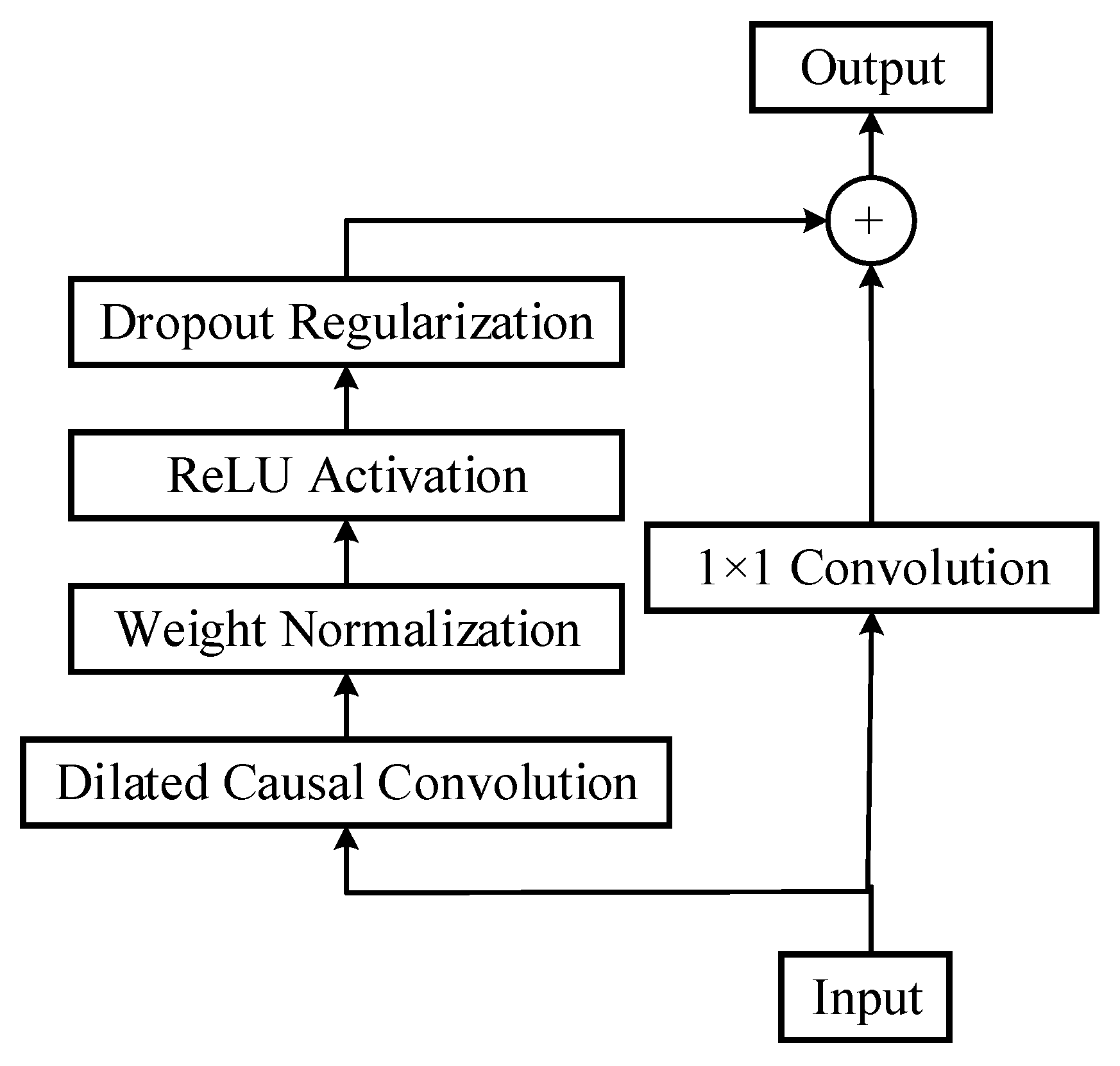
The Temporal Convolutional Network (TCN) is a deep learning architecture designed for modeling time-series data. It utilizes causal convolutions combined with dilated convolutions to effectively model sequential dependencies. Unlike traditional convolutional neural networks, TCN modifies the convolution operations to ensure causality—that is, the output at any time step depends only on current and past inputs, preventing information leakage from the future. This design enables TCNs to efficiently capture long-range temporal dependencies in sequential data. The dilated causal convolution structure of the TCN is illustrated in Figure 1 [23].
A causal convolution ensures that the output at time step t depends only on inputs from time steps ≤ t. This avoids the “information leakage” problem. Formally:
y t = i = 0 k 1 ω i x t i
where k is the kernel size, and ω i are convolution weights.
To enlarge the receptive field without increasing computational cost, dilated convolution introduces a dilation factor d:
y t = i = 0 k 1 ω i x t d i
Thus, the receptive field grows exponentially with depth, allowing the TCN to capture long-range dependencies. Furthermore, residual blocks are employed to stabilize gradient propagation:
H ( x ) = σ ( W x + b ) + x
where H(x) is the block output, σ is the activation function, and W x denotes convolution. This architecture improves convergence and enhances forecasting accuracy. Figure 2 illustrates the basic architecture of the TCN model, which is built upon the dilated causal convolution. The architecture further incorporates weight normalization layers, ReLU activation functions, and dropout layers to enhance training stability, introduce non-linearity, and prevent overfitting, respectively.

2.4. iTransformer Model

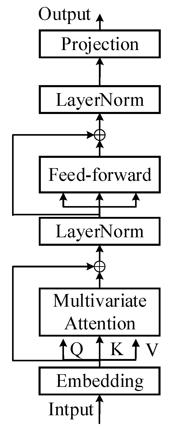
The iTransformer is an architectural variant based on the traditional Transformer model, which has demonstrated excellent performance in fields such as natural language processing and computer vision [20]. However, conventional Transformer structures often suffer from high computational complexity and entangled variable representations, leading to relatively suboptimal performance in time series forecasting tasks. By inverting the input of the traditional Transformer structure, the iTransformer achieves improved generalization, computational efficiency, and predictive accuracy. As illustrated in Figure 3, the iTransformer architecture comprises the following functions: embedding layer, multivariate attention mechanism, feed-forward network, layer normalization, and projection layer.
As illustrated in Figure 3, the iTransformer architecture comprises the following functions: embedding layer, multivariate attention mechanism, feed-forward network, layer normalization, and projection layer. In the attention mechanism, the Query (Q), Key (K), and Value (V) matrices are obtained by linear transformations of the embedded input sequence. Specifically, Q represents the feature vector used to match relevant information, K represents the feature vector that provides the reference for matching, and V represents the feature vector that carries the actual information to be aggregated. The attention weights are computed by measuring the similarity between Q and K, and then, used to weigh the corresponding V for feature extraction and prediction.

2.4.1. Embedding Layer

Given a time series with T time steps, denoted as X = { x 1 , x 2 , , x T } , the embedding layer maps each variable sequence through an embedding function into a D-dimensional embedding vector:
h n 0 = E m b e d d i n g ( X : , n )
wherein X : , n denotes the entire time series corresponding to the n-th variable of the input sequence X.

2.4.2. Multi-Head Attention Mechanism

This layer captures dependencies among features by applying self-attention to each variable’s time series. For each embedded time series H 1 = { h 1 , , h n } obtained from the embedding layer, linear transformations are performed to generate the Query (Q), Key (K), and Value (V) matrices [27]:
A t t e n t i o n ( Q , K , V ) = S o f t m a x ( Q K T d k ) V
h e a d i = A t t e n t i o n ( H l 1 W Q l , H l 1 W K l , H l 1 W V l )
M u l t i H e a d ( H l 1 ) = [ h e a d 1 ; ; h e a d h ] W O
where W Q l , W K l , W V l denote the weight matrices used in the attention mechanism.

2.4.3. Feed-Forward Network

This layer applies nonlinear activation functions and regularization mechanisms to the output variables M u l t i H e a d ( H l 1 ) from the attention mechanism, thereby capturing independent temporal patterns for each variable in the time series:
H l = F E N ( M u l t i H e a d ( H l 1 ) )
F E N ( M u l t i H e a d ( H l 1 ) ) = σ ( M u l t i H e a d ( H l 1 ) W 1 + b 1 ) W 2 + b 2
Here, W denotes the weight matrix, b represents the bias term, and σ ( ) is the nonlinear activation function.

2.4.4. Layer Normalization

This layer applies normalization to the input variable’s time series representations, reducing differences caused by varying measurement units or distribution discrepancies among variables:
L a y e r N o r m ( H ) = H M e a n ( H ) V a r ( H )

2.4.5. Projection Layer

This layer maps the input variable H l of dimension D to the target number of prediction time steps and outputs the final prediction results Y ^ : , n :
Y ^ : , n = P r o j e c t i o n ( H : , n l )
P r o j e c t i o n ( H : , n l ) = H : , n l W p + b p

3. RIME-VMD-TCN-iTransformer Hybrid Model

3.1. VMD Optimized by RIME

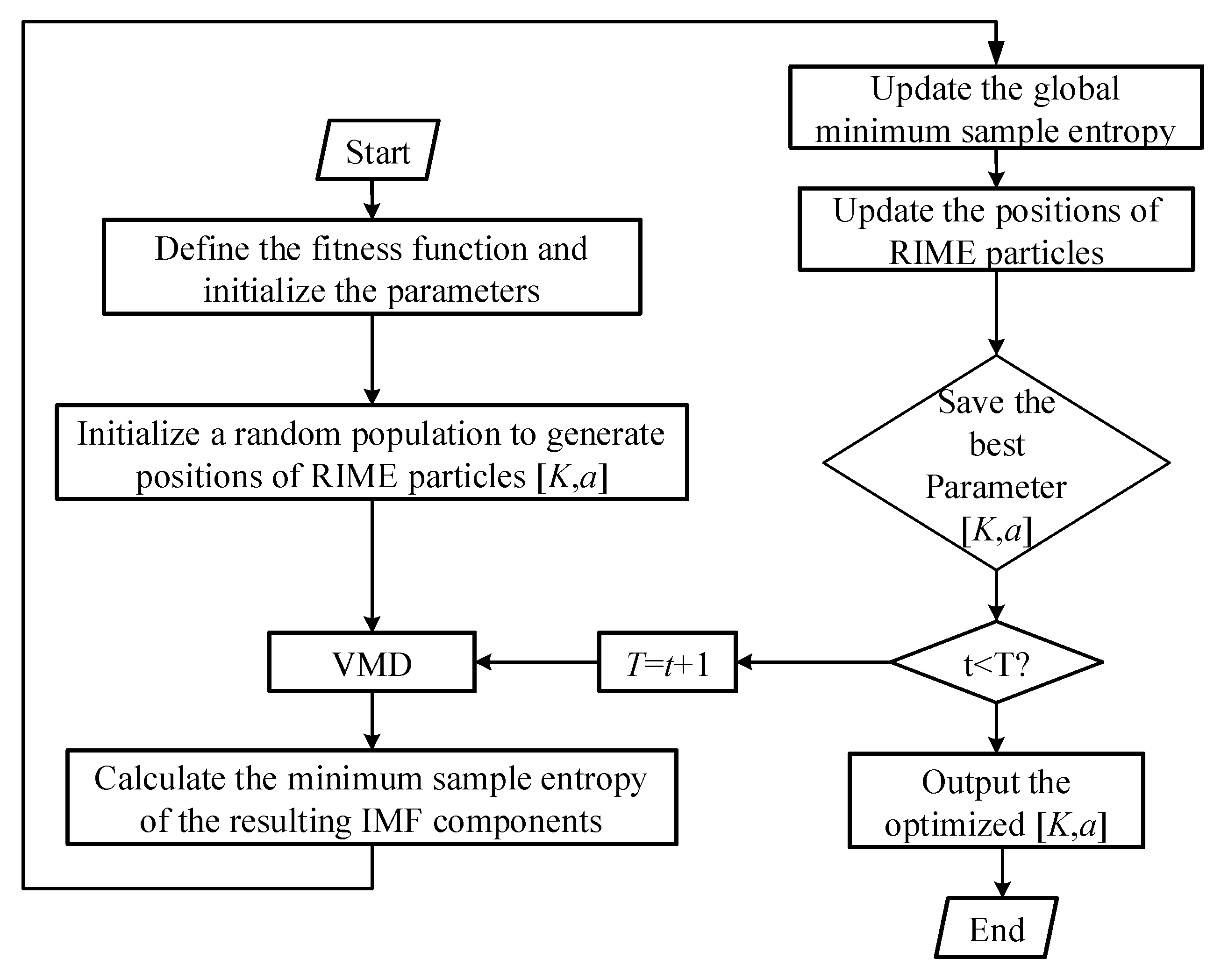
Since the decomposition number K and penalty factor α significantly influence the decomposition results of VMD, this study employs the RIME to optimize the selection of K and α . The optimization objective is defined using sample entropy, which effectively reflects the dynamic patterns of the time series. Sample entropy evaluates the complexity of the time series and accurately characterizes the relationship between each subsequence and the original time series [19]. The calculation of sample entropy is performed as follows: each intrinsic mode function is reconstructed into an m-dimensional sequence vector X m ( 1 ) , , X m ( N m 1 ) , where X m ( i ) = { x ( i ) , x ( i + 1 ) , , x ( i m + 1 ) } . Define the distance d [ X m ( i ) , X m ( j ) ] between two different vectors as the maximum absolute difference [11]:
d [ X m ( i ) , X m ( j ) ] = max ( x ( i + k ) x ( j + k ) )
Based on the proportion of matching between two subsequences, the tolerance r is defined as the distance threshold between X m ( i ) and X m ( j ) . For a given X m ( i ) , the matching degree B i between X m ( i ) and other subsequences is computed as the proportion of subsequences whose distance to X m ( i ) is less than or equal to r:
B i m ( r ) = B i N m 1
Accordingly, the sample entropy is defined as
S a m p E n ( m , r , N ) = ln i = 1 N m B i m ( r ) i = 1 N m + 1 B i m + 1 ( r )
A higher sample entropy value between two sequences indicates greater randomness and irregularity in the time series, while a lower sample entropy value suggests the sequence is more regular and predictable. By minimizing the sample entropy of each function as the objective function, the optimization process is illustrated in Figure 4.

3.2. TCN-iTransformer Prediction Model

To address nonlinear and stochastic fluctuations in transformer load, the proposed RIME-VMD-TCN-iTransformer model integrates decomposition, optimization, and deep learning. First, the VMD algorithm decomposes the raw sequence into multiple IMFs, thereby reducing non-stationarity. Then, the RIME adaptively determines the optimal decomposition parameters, ensuring stability and minimizing random noise. The TCN extracts local nonlinear dynamics through dilated causal convolutions, while the iTransformer captures global correlations and stochastic variations by modeling inter-variable dependencies across time. This integrated design enables the model to remain robust in predicting abrupt load peaks and long-term fluctuations. The architecture of the model is illustrated in Figure 5.

3.3. Prediction Process

The prediction process of the RIME-VMD-TCN-iTransformer model is as follows:
  • Preprocess the raw data by removing outliers and handling missing values [21,22,23];
  • Obtain IMFs via VMD optimized by RIME;
  • Construct separate TCN-iTransformer prediction models for each IMFs, and update the network parameters using the adam optimizer;
  • Reconstruct the prediction by aggregating the forecasting results of all IMFs.

3.4. Evaluation Parameters

To evaluate the performance of different dissolved gas prediction models, this study adopts mean absolute percentage error (MAPE), root mean square error (RMSE) and coefficient of determination (R2) as evaluation criteria. Their calculation formulas are given by
M A P E = 1 n i = 1 n y i y i y i × 100 % f
R M S E = 1 n i = 1 n ( y i y i ) 2
R 2 = 1 i = 1 n ( y i y ^ i ) 2 i = 1 n ( y i y ¯ i ) 2
where n is the number of testing samples, y i and y i represent the true and predicted load of power transformer at time step i, respectively.
This study employs the PyTorch 2.2.0 framework to build the prediction model. For the TCN, the convolution kernel size is set to 4, the number of hidden layers is set to 4, the number of attention heads was set to 8, the attention factor was 5, and the GeLU activation function was employed. The iTransformer model uses an attention dimension of 128 and a dropout rate of 0.1. The training process updates model parameters using the adam optimizer, with 200 training epochs and a learning rate of 0.001. The hardware platform for training consists of an Intel Xeon (R) Platinum 8255C CPU and an RTX 2080 Ti (22 GB) GPU.
This study employs the PyTorch framework to build the prediction model. The hyperparameters used in this study were determined through preliminary experiments and reference to related literature. Specifically, the convolution kernel size of the TCN was set to 4 to balance the receptive field and computational efficiency, while four hidden layers were adopted to capture sufficient temporal dependencies without overfitting. The number of attention heads was set to 8, and the attention factor to 5, following common practice in multivariate time series forecasting to ensure stable convergence. The iTransformer attention dimension was set to 128 to provide sufficient feature representation capacity. A dropout rate of 0.1 was chosen to avoid overfitting while maintaining training stability. The learning rate was fixed at 0.001 with 200 training epochs, which achieved stable convergence in preliminary validation experiments. The hardware platform for training consists of an Intel Xeon (R) Platinum 8255C CPU and an RTX 2080 Ti (22 GB) GPU. The definitions of symbols and abbreviations used in this study are listed in Appendix A.

4. Case Study

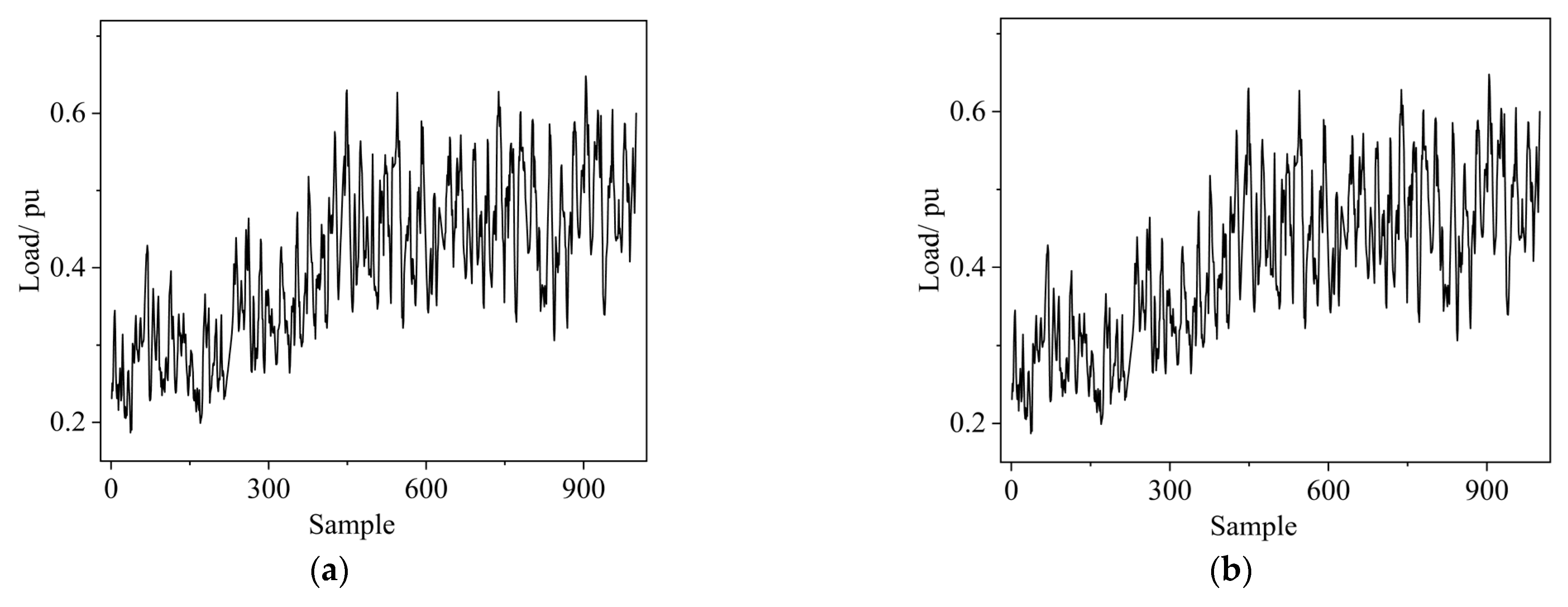
This study employs the load data of six transformers from the Hebei Baoding substation for model validation. Each dataset covers the period from 24 April to 4 June 2024, with a one-hour sampling interval, yielding about 1000 data points per transformer. As shown in Figure 6, the load of the #1 1050 kV transformer displays an overall increasing trend along with local periodic fluctuations, reflecting daily electricity consumption cycles. For model development, the first 80% of the data is used for training, and the remaining 20% is used for testing.
Before model training, the raw transformer load data underwent several preprocessing steps. First, abnormal points were identified and removed using the 3σ criterion to eliminate the influence of outliers. Then, min–max normalization was applied to scale all values into the range (−1, 1), thereby reducing magnitude differences and improving convergence during training. Finally, the normalized time series was segmented into input–output pairs with a rolling window of 10 days, where the data from days 1–10 was used to predict day 11, days 2–11 to predict day 12, and so forth. This preprocessing pipeline ensured data quality and consistency in forecasting tasks.

4.1. Prediction Results of the RIME-VMD-TCN-iTransformer Model

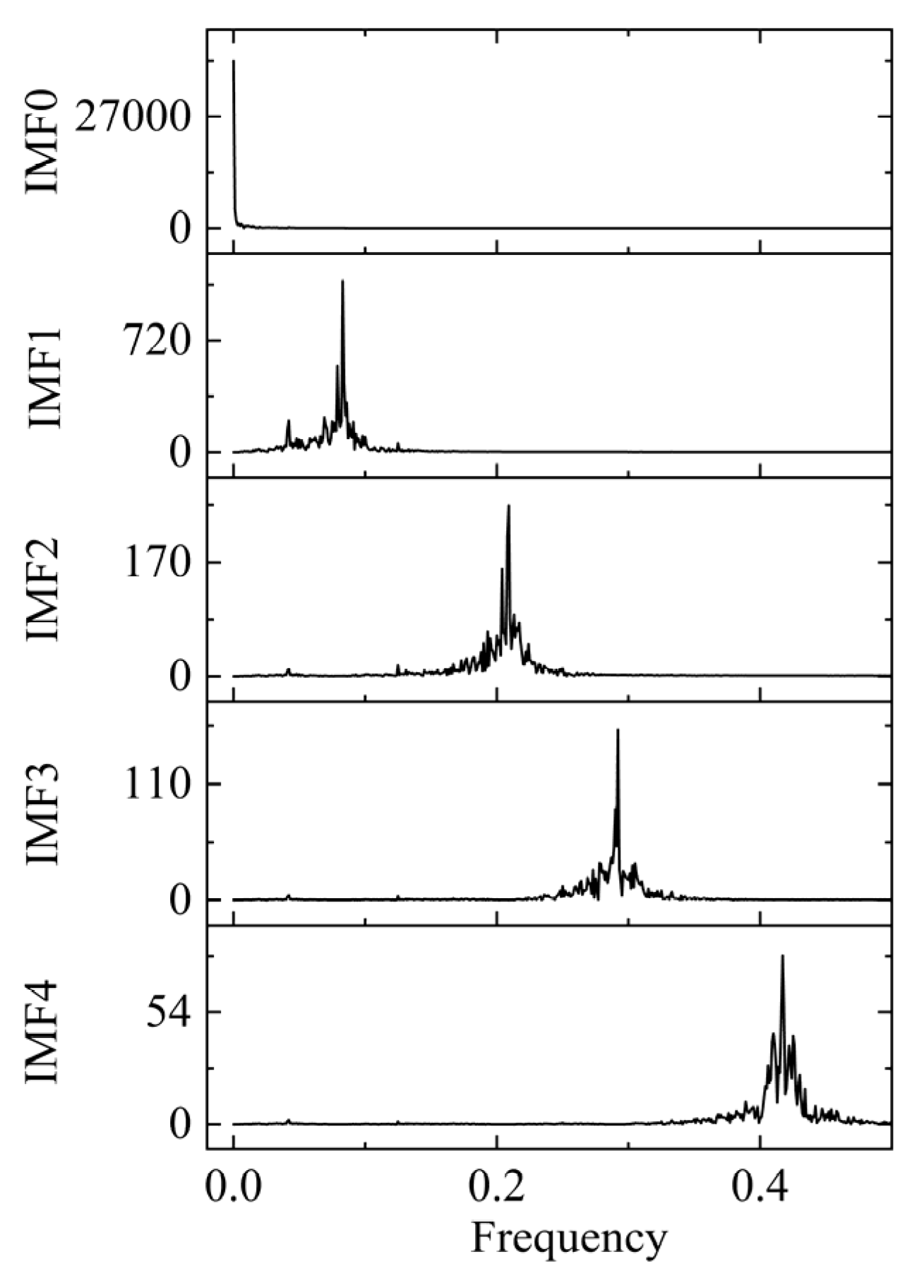
Based on the optimal number of modal decompositions K = 5 and penalty term a = 1, the decomposition parameters obtained from RIME-VMD are presented in Figure 7, where the time series is decomposed into five functions with concentrated frequency bands, and no spectral aliasing is observed among the IMF. The stationary and regular modal decomposition effectively reduces the complexity of subsequent prediction modeling, providing a strategy to address the nonlinearity and nonstationary of transformer load forecasting.
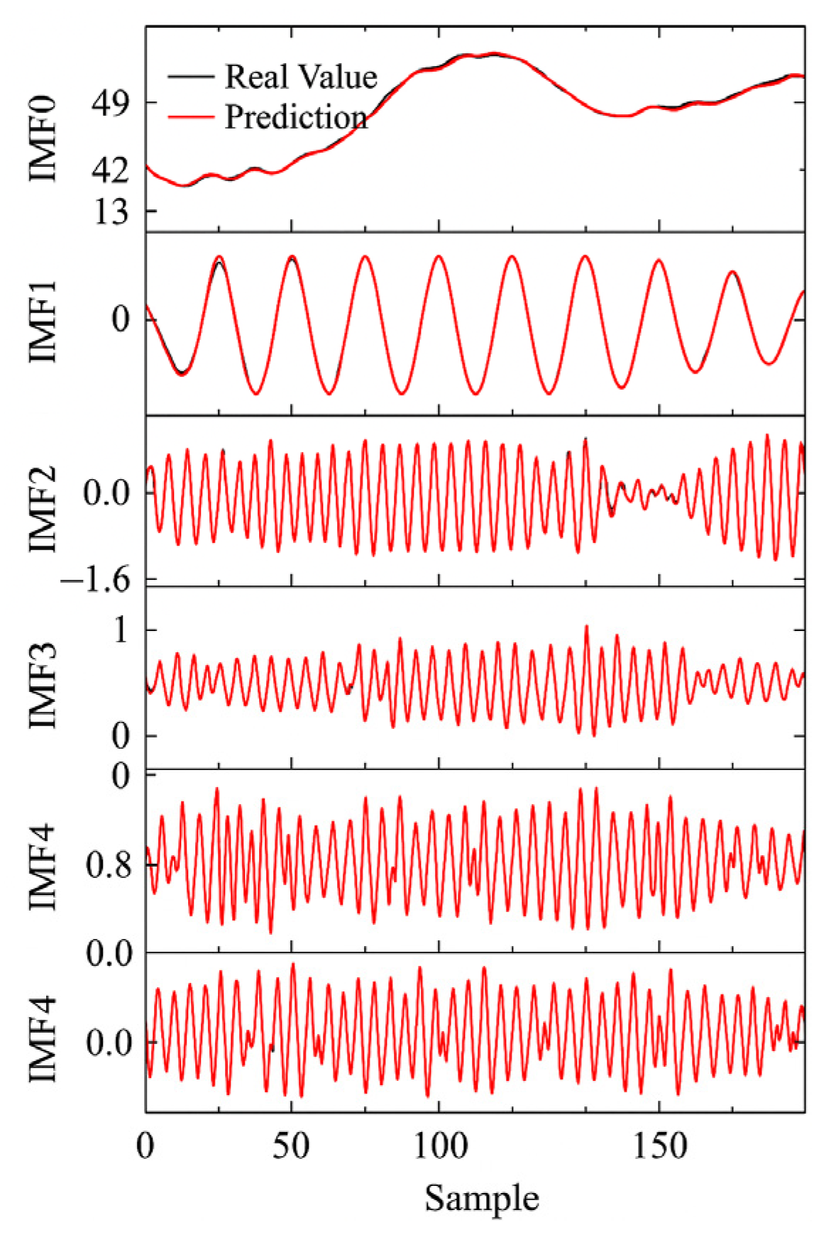
The decomposed data were normalized and subsequently fed into the optimal TCN-iTransformer model for training. The forecasting results of each IMFs of the transformer load are shown in Figure 8. The proposed TCN-iTransformer model demonstrates a high degree of agreement between the predicted values and the actual observations for each sub-sequence obtained through RIME-VMD, further confirming that RIME-VMD enhances prediction accuracy by mitigating the nonlinearity of the original signal.
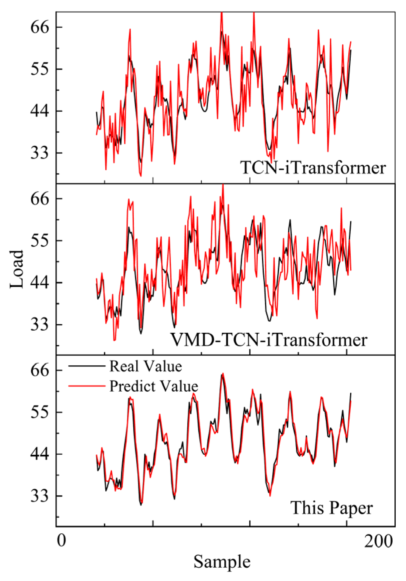
The reconstructed original time series obtained by aggregating all IMFs is shown in Figure 9. The proposed model responds promptly even when the signal exhibits significant fluctuations. To further validate the advantages of the proposed approach, comparative analyses were conducted with two benchmark models: one directly predicting based on the original signal (i.e., the TCN-iTransformer model), and the other employing a non-optimized decomposition process (i.e., the VMD-TCN-iTransformer model). All models were trained using identical parameter settings as those applied in the proposed model. The comparison results and evaluation metrics of the respective models are presented in Figure 9 and Table 1.
As shown in Figure 9, the proposed model achieves prediction results much closer to the actual values than the benchmark models. This performance improvement can be attributed to two key factors. First, the decomposition–prediction–reconstruction framework optimized by RIME effectively eliminates spectral aliasing and enhances the orderliness of the modal functions, making each sub-sequence more predictable. Second, the TCN-iTransformer model integrates the advantages of convolution in capturing local temporal dependencies and the inverted Transformer in modeling long-range correlations, which enables more accurate forecasting of both long-term trends and abrupt fluctuations. In contrast, the baseline models either lack decomposition optimization or fail to capture multiscale temporal dependencies, resulting in higher prediction errors.
The predicted values based on the TCN-iTransformer model fail to capture the large-scale periodic fluctuations observed in the actual values, resulting in relatively higher prediction errors, with MAPE and RMSE of 8.302% and 4.897, respectively. When the original signal is first decomposed using VMD prior to prediction, the forecasting performance is significantly improved, with the prediction errors reduced by 42.98% and 23.42%, respectively, indicating that VMD effectively mitigates the non-stationarity of the original data. The separate forecasting of long-term and short-term functions extracted by VMD further contributes to enhancing the prediction accuracy. In our model, the decomposition process was further optimized by integrating the RIME, thereby improving the separability of the modal functions. The concentrated distribution of modal functions suggests that the decomposed sequences exhibit stronger regularity, which is also a key factor in improving the model’s prediction accuracy. The optimized model achieves MAPE and RMSE of 2.23% and 1.161, respectively, representing more than a threefold reduction in prediction errors compared to the direct forecasting of the original signal. In addition, the R2 value of our model is closer to 1, further indicating that the prediction results effectively capture the variation trends of the load.

4.2. Generalization Ability Analysis

To further validate the effectiveness of our model, transformer load forecasting was also conducted for other transformers with different capacities and groups at Baoding Station in Hebei Province. The detailed prediction results are presented in Table 2. Compared with the original time series signal and the non-optimized modal decomposition method, the proposed model consistently achieved the best error evaluation metrics across all datasets, further demonstrating its superior prediction accuracy and strong generalization capability.

5. Conclusions

In this study, we proposed a hybrid transformer load forecasting model based on RIME-VMD and TCN-iTransformer. The main conclusions can be summarized as follows:
(1)
Methodological Contribution: By integrating variational mode decomposition (VMD) with the randomized improved marine predators algorithm (RIME), the proposed framework effectively eliminates spectral aliasing and enhances the orderliness of intrinsic mode functions (IMFs). This improves the interpretability of decomposed components for load forecasting tasks.
(2)
Model Performance: The hybrid TCN-iTransformer model combines the advantages of convolutional layers for capturing short-term local dependencies and the inverted Transformer for modeling long-term global correlations. Experimental results on 1000 kV transformer datasets demonstrate that our model achieves superior accuracy compared with benchmark methods, with significantly reduced MAPE and RMSE values.
(3)
Practical Implications: The proposed model provides a reliable tool for predicting both abrupt fluctuations and long-term load trends, enabling power utilities to optimize transformer operation, reduce the risk of overload, and prevent potential failures. This is significant for ensuring the safety and stability of large-scale power systems.
Future research will extend the methodology to other types of substation equipment, incorporate physical constraints into the neural framework, and validate the approach on larger-scale, multi-regional datasets.

Author Contributions

Writing—original draft preparation, Y.Z.; Writing—review and editing, Y.Z., C.X., Y.Y. and S.G.; Collecting the samples, Y.Z.; Software and data processing, Y.Z., H.L., L.D. and T.Z.; Funding acquisition, C.X. All authors have read and agreed to the published version of the manuscript.

Funding

This research was supported by the Science and Technology Project of State Grid Hebei Electric Power Co., Ltd. (kj2024-029).

Data Availability Statement

The data presented in this study are available on request from the corresponding author. The data are not publicly available due to confidentiality agreements with the State Grid Corporation of China and data privacy restrictions.

Conflicts of Interest

The authors declare no conflict of interest.

Appendix A

Table A1. List of Symbols and Abbreviations.
Symbol/AbbreviationDefinition/Full FormNotes
X = { x 1 , , x T } Original time seriesT: length of sequence
DEmbedding dimension
Q, K, VQuery, Key, Value matricesAttention mechanism
W, bWeight matrix and bias term
f ( ) Nonlinear activation functione.g., GeLU
KNumber of modes in VMD
aPenalty factor in VMD
IMFkk-th intrinsic mode function
mEmbedding dimension for entropy
rTolerance (threshold)Sample entropy
d ( ) Distance function
Φ Matching degree
SEnSample entropy
y ^ i True/predicted load
MAPEMean Absolute Percentage Error
RMSERoot Mean Square Error
R2Coefficient of determination
VMDVariational Mode Decomposition
RIMERandomized Improved Marine Predators AlgorithmOptimization
TCNTemporal Convolutional Network
IMFIntrinsic Mode Function
DGADissolved Gas AnalysisIf mentioned
SGCCState Grid Corporation of China

References

  1. IEEE Std C57.91-2011; IEEE Guide for Loading Mineral-Oil-Immersed Transformers and Step-Voltage Regulators. IEEE: Piscataway, NJ, USA, 2011.
  2. Biçen, Y.; Aras, F.; Kirkici, H. Lifetime estimation and monitoring of power transformer considering annual load factors. IEEE Trans. Dielectr. Electr. Insul. 2014, 21, 1360–1367. [Google Scholar] [CrossRef]
  3. Paterakis, N.G.; Pappi, I.N.; Erdinc, O.; Godina, R.; Rodrigues, E.M.G.; Catalao, J.P.S. Consideration of the impacts of a smart neighborhood load on transformer aging. IEEE Trans. Smart Grid 2015, 7, 2793–2802. [Google Scholar] [CrossRef]
  4. Huang, W.; Shao, C.; Dong, M.; Hu, B.; Zhang, W.; Sun, Y.; Xie, K.; Li, W. Modeling the aging-dependent reliability of transformers considering the individualized aging threshold and lifetime. IEEE Trans. Power Del. 2022, 37, 4631–4645. [Google Scholar] [CrossRef]
  5. Othman, N.A.; Zainuddin, H.; Yahaya, M.S.; Azis, N.; Ibrahim, Z. Prerequisites for accelerated aging of transformer oil: A review. IEEE Trans. Dielectr. Electr. Insul. 2024; in press. [Google Scholar]
  6. Jiang, P.; Zhang, Z.; Dong, Z.; Yang, Y.; Pan, Z.; Yin, F.; Qian, M. Transient-steady state vibration characteristics and influencing factors under no-load closing conditions of converter transformers. Int. J. Electr. Power Energy Syst. 2024, 155, 109497. [Google Scholar] [CrossRef]
  7. Gui, F.; Chen, H.; Zhao, X.; Pan, P.; Xin, C.; Jiang, X. Enhancing economic efficiency: Analyzing transformer life-cycle costs in power grids. Energies 2024, 17, 606. [Google Scholar] [CrossRef]
  8. Okeke, R.O.; Ibokette, A.I.; Ijiga, O.M.; Enyejo, L.A.; Ebiega, G.I.; Olumubo, O.M. The reliability assessment of power transformers. Eng. Sci. Technol. J. 2024, 5, 1149–1172. [Google Scholar] [CrossRef]
  9. Xie, X.; Qian, T.; Li, W.; Tang, W.; Xu, Z. An individualized adaptive distributed approach for fast energy-carbon coordination in transactive multi-community integrated energy systems considering power transformer loading capacity. Appl. Energy 2024, 375, 124189. [Google Scholar] [CrossRef]
  10. Zhu, L.; Gao, J.; Zhu, C.; Deng, F. Short-term power load forecasting based on spatial-temporal dynamic graph and multi-scale transformer. J. Comput. Des. Eng. 2025, 12, 92–111. [Google Scholar] [CrossRef]
  11. Hyndman, R.J.; Athanasopoulos, G. Forecasting: Principles and Practice, 3rd ed.; OTexts: Ontario, ON, Canada, 2021. [Google Scholar]
  12. Wang, N.; Li, W.; Li, J.; Li, X.; Gong, X. Prediction of dissolved gas content in transformer oil using the improved SVR model. IEEE Trans. Appl. Supercond. 2024, 34, 1205–1211. [Google Scholar] [CrossRef]
  13. Breiman, L. Random forests. Mach. Learn. 2001, 45, 5–32. [Google Scholar] [CrossRef]
  14. Huang, G.; Zhou, H.; Ding, X.; Zhang, R. Extreme learning machine for regression and multiclass classification. IEEE Trans. Syst. Man Cybern. B 2012, 42, 513–529. [Google Scholar] [CrossRef]
  15. Qiu, X.; Ren, Y.; Suganthan, P.N.; Amaratunga, G.A.J. Empirical mode decomposition based ensemble deep learning for load demand forecasting. Appl. Soft Comput. 2017, 54, 246–255. [Google Scholar] [CrossRef]
  16. Wu, Z.; Huang, N.E. Ensemble empirical mode decomposition: A noise-assisted data analysis method. Adv. Adapt. Data Anal. 2009, 1, 1–41. [Google Scholar] [CrossRef]
  17. Dragomiretskiy, K.; Zosso, D. Variational mode decomposition. IEEE Trans. Signal Process. 2014, 62, 531–544. [Google Scholar] [CrossRef]
  18. Li, Q.; Zhang, X.; Ma, T.; Ma, T.; Wang, H.; Yin, H. Ultra-short-term multi-step wind power forecasting based on ECBO-VMD-WKELM. Power Syst. Technol. 2021, 45, 3070–3080. [Google Scholar]
  19. Kennedy, J.; Eberhart, R. Particle swarm optimization. In Proceedings of the IEEE ICNN, Perth, Australia, 9–12 June 1995; pp. 1942–1948. [Google Scholar]
  20. Yuan, Y.; Huang, K.; Chen, J.; Bao, L.; Zhou, Q. Research on fault diagnosis method of on-load tap changer based on WSO-VMD sample entropy and SSA-SVM. J. Southwest Univ. 2024, 46, 203–216. [Google Scholar]
  21. Mirjalili, S.; Mirjalili, S.M.; Lewis, A. Grey wolf optimizer. Adv. Eng. Softw. 2014, 69, 46–61. [Google Scholar] [CrossRef]
  22. Hochreiter, S.; Schmidhuber, J. Long short-term memory. Neural Comput. 1997, 9, 1735–1780. [Google Scholar] [CrossRef]
  23. Bai, S.; Koltun, V.; Kolter, J.Z. An empirical evaluation of generic convolutional and recurrent networks for sequence modeling. arXiv 2018, arXiv:1803.01271. [Google Scholar] [CrossRef]
  24. Huy, P.C.; Minh, N.Q.; Tien, N.D.; Anh, T.T.Q. Short-term electricity load forecasting based on temporal fusion transformer model. IEEE Access 2022, 10, 106296–106304. [Google Scholar] [CrossRef]
  25. Liu, Y.; Hu, T.; Zhang, H.; Wu, H.; Wang, S.; Ma, L.; Long, M. iTransformer: Inverted transformers are effective for time series forecasting. arXiv 2023, arXiv:2308.12345. [Google Scholar]
  26. Su, H.; Zhao, D.; Heidari, A.; Liu, L.; Zhang, X.; Mafarja, M.; Chen, H. RIME: A physics-based optimization. Neurocomputing 2023, 532, 183–214. [Google Scholar] [CrossRef]
  27. Richman, J.S.; Moorman, J.R. Physiological time-series analysis using approximate entropy and sample entropy. Am. J. Physiol. Heart Circ. Physiol. 2000, 278, H2039–H2049. [Google Scholar] [CrossRef]
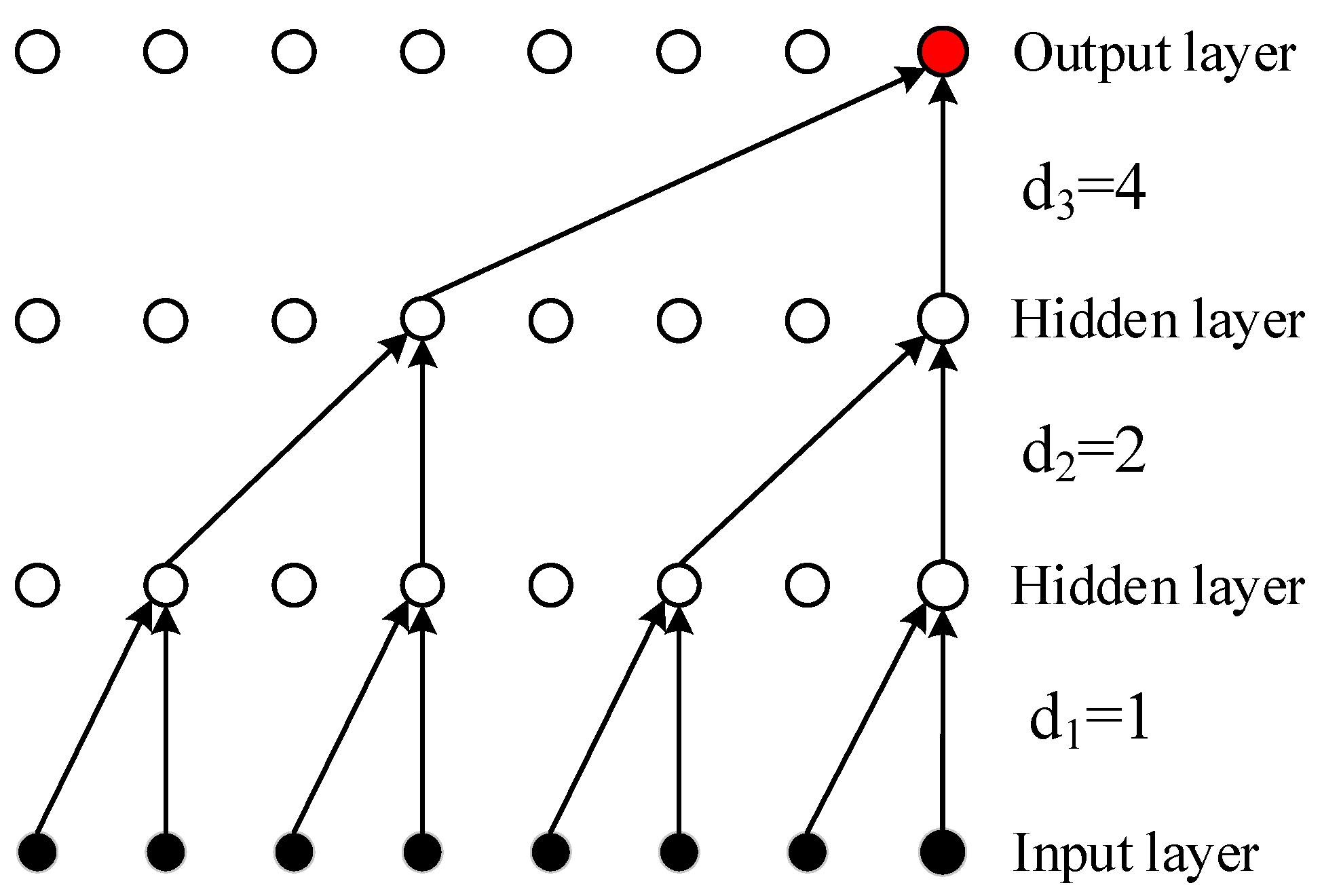
Figure 1. Extended causal convolution structure.
Applsci 15 11241 g001
Figure 2. Structure of TCN.
Applsci 15 11241 g002
Figure 3. Structure of iTransformer.
Applsci 15 11241 g003
Figure 4. Flowchart of RIME-optimized VMD.
Applsci 15 11241 g004
Figure 5. Structure of TCN-iTransformer.
Applsci 15 11241 g005
Figure 6. Time series results of transformer load. (a) total sequence, (b) partial sequence.
Applsci 15 11241 g006
Figure 7. Frequency spectrum of load sequence decomposed by RIME-VMD method.
Applsci 15 11241 g007
Figure 8. Prediction results of all IMFs.
Applsci 15 11241 g008
Figure 9. Comparison of the prediction results with different models.
Applsci 15 11241 g009
Table 1. Prediction error of different models.
ModelMAPERMSER2
TCN-iTransformer8.302%4.89756.71%
VMD-TCN-iTransformer4.733%3.76974.32%
This paper2.23%1.16193.71%
Table 2. Comparison of prediction results in different transformer types.
Transformer TypeEvaluation MetricsModel
TCN-iTransformerVMD-TCN-iTransformerThis Paper
2: 1000 kVMAPE4.917%3.431%2.917%
RMSE9.4835.5483.983
R20.7120.8660.918
1: 500 kVMAPE3.923%3.012%1.923%
RMSE9.7876.6913.427
R20.6980.6120.927
2: 500 kVMAPE3.790%2.618%1.790%
RMSE10.2379.3266.237
R20.4560.6130.924
1: 110 kVMAPE5.191%3.789%2.291%
RMSE4.7822.6511.782
R20.7120.8120.956
2: 110 kVMAPE5.191%3.789%2.291%
RMSE4.7822.6511.782
R20.6710.7520.913
Disclaimer/Publisher’s Note: The statements, opinions and data contained in all publications are solely those of the individual author(s) and contributor(s) and not of MDPI and/or the editor(s). MDPI and/or the editor(s) disclaim responsibility for any injury to people or property resulting from any ideas, methods, instructions or products referred to in the content.