Article

Driving Mechanisms of Urban Form on Anthropogenic Carbon Emissions: An RSG-Net Ensemble Model for Targeted Carbon Reduction Strategies

1
School of Architecture and Urban Planning, Anhui Jianzhu University, Hefei 230009, China
2
School of Environmental and Energy Engineering, Anhui Jianzhu University, Hefei 230601, China
3
College of Geoexploration Science and Technology, Jilin University, Changchun 130026, China
*
Author to whom correspondence should be addressed.
Appl. Sci. 2025, 15(20), 11175; https://doi.org/10.3390/app152011175
Submission received: 17 September 2025 / Revised: 16 October 2025 / Accepted: 17 October 2025 / Published: 18 October 2025
(This article belongs to the Section Environmental Sciences)

Abstract

Urban Form (UF), as a synthesis of urban functions and socioeconomic elements, is closely associated with Anthropogenic Carbon Emissions (ACE) and has important implications for low-carbon urban planning. As a key national economic strategy region, the Yangtze River Economic Belt (YREB) exhibits pronounced heterogeneity in urban development, highlighting the urgent need to elucidate the interaction mechanisms between UF and ACE to support carbon reduction strategies. This study employs nighttime light data and carbon emission records from 2002 to 2022 in the YREB. By integrating Support Vector Regression (SVR), Random Forest (RF), and Gradient Boosting Decision Tree (GBDT), we developed a neural network ensemble model (RSG-Net) to analyze the impacts and driving mechanisms of UF on ACE. The results indicate the following: (1) Over the past two decades, total ACE in the YREB increased by 196%, displaying a three-phase trajectory of rapid growth, deceleration, and rebound. (2) The RSG-Net model achieved superior predictive performance, with an R2 of 0.93, an RMSE of 1.96 × 10⁶ t, an RPD of 3.69, and a PBIAS of 4.53%. (3) Based on Pearson correlation analysis and SHAP (Shapley Additive Explanations) feature importance, beyond economic and demographic indicators, the most influential UF indicators are ranked as Number of Urban Patches (NP), Normalized Difference Vegetation Index (NDVI), and Construction Land Concentration (CLC). These findings demonstrate that the RSG-Net model can not only predict ACE but also identify key UF factors and explain their interrelationships, thereby providing technical support for the formulation of urban carbon reduction strategies.

1. Introduction

Urban areas, while occupying only 2.8% of the Earth’s land surface, account for 70.8% of global energy-related CO2 emissions, exerting a profound influence on global environmental change [1]. In the process of urbanization, Urban Form (UF) represents a key quantifiable dimension, as it captures the overall spatial configuration of the built environment and its dynamic interactions with socioeconomic factors [2]. The continued expansion of anthropogenic activities has positioned urban areas as the primary source of greenhouse gas emissions, with Anthropogenic Carbon Emissions (ACE) constituting the most significant component [3,4]. Therefore, clarifying the relationship between ACE and UF, as well as identifying critical urban morphological characteristics, is essential for enabling precise carbon mitigation at the city scale.
Empirical studies indicate that anthropogenic factors such as population size, economic structure, and road transportation significantly influence urban CO2 emission patterns [5,6,7]. For example, Du et al. showed that controlling population and economic growth reduces aggregate carbon emissions, while limiting energy use in secondary industries lowers urban emissions [8]. Xie et al. further revealed that transportation infrastructure contributes to higher emissions by stimulating economic growth and promoting technological innovation [9]. Urban land-use configurations significantly influence CO2 emissions, with spatial econometric approaches frequently employed to quantify the effects of land-use patterns and spatial structures on emission dynamics at the city scale [10,11]. Although much of the existing literature tends to examine the drivers of urban carbon emissions in isolation, Bereitschaft and Debbage found that a comprehensive analysis of the spatial distribution of urban buildings, roads, infrastructure, resources, and population density can effectively assess the impact of urban form on CO2 emissions [12]. For example, Shi et al. applied geographically and temporally weighted regression analysis to 256 Chinese cities, finding that urban form correlates positively with economic factors but negatively with social indicators [13]. Ding et al. combined the STIRPAT model with threshold regression, revealing a nonlinear inverse relationship between urban compactness and emissions, with dual-threshold effects [14]. Collectively, these studies indicate that traditional methods have limitations in capturing nonlinear responses, variable interactions, and higher-order correlations in the analysis of the UF-CO2 emission nexus.
Machine learning outperforms traditional models in capturing complex nonlinear relationships via adaptive learning, demonstrates enhanced robustness and generalization, and shows substantial promise for investigating the linkage between urban form and CO2 emissions. As indicated by Wu and Li, gradient boosted decision trees were used to quantify the impact of urban form, which accounts for 31.32% of the predictive capacity for transport emissions [15]. Although machine learning applications in UF-ACE systems are currently scarce, they are well-established in related urban environmental research domains. For example, Li et al. applied the Support Vector Machine (SVM) algorithm to analyze urban element indicators, showing that SVM outperformed the linear regression model with an R2 of 0.46 and an RMSE of 0.91 [16].
Ensemble learning is an advanced machine learning approach that integrates complementary strengths from various base models [17]. As demonstrated by Chaturvedi and De Vries [18], a multi-model collaborative framework can leverage the complementary capabilities of different algorithms: Random Forest (RF) for high-dimensional feature selection, Support Vector Machines (SVM) for nonlinear fitting, and Gradient Boosting Decision Trees (GBDT) for deep feature extraction. This method exhibits strong predictive power, as shown by Xing et al., who used an RF ensemble model to predict the emission levels of various urban air pollutants, all with R2 values exceeding 0.94 [19]. Jiang et al. developed an ensemble model for building a CO2 prediction that achieved 96.3% accuracy, outperforming traditional models such as linear regression and decision trees [20]. Requia et al. and Yan et al. revealed that ensemble learning, by integrating diverse base learners, enhances model robustness and adaptability in complex and heterogeneous environments, enabling the effective capture of nonlinear relationships and spatial heterogeneity compared with single-model approaches [21,22]. Therefore, this study adopts an ensemble learning framework to more accurately characterize carbon emission patterns across the YREB, a region distinguished by its vast spatial span and diverse urban morphology. Despite the limited direct application to the UF–ACE nexus, the proven track record of ensemble learning in similar urban–environmental contexts justifies its use in this investigation.
Based on the above, this paper focuses on the Yangtze River Economic Belt (YREB) as the study area, integrating multi-source nightlight data, ODIAC data, socioeconomic statistics, and other datasets to construct a long-term time series ACE dataset and a multi-dimensional morphological indicator set for the period 2002–2022. Additionally, the RSG-Net integrated framework is proposed, which synergistically combines support vector regression (SVR), gradient boosting decision trees (GBDT), random forest (RF), and the SHAP method to analyze the relationship between UF and ACE. The principal objectives are to (1) reconstruct ACE and delineate urban built-up areas through multi-source data integration, elucidating regional ACE spatiotemporal dynamics and quantifying UF driving mechanisms; and (2) by optimizing the performance of the RSG-Net model, this study reveals the association mechanism between UF and ACE, establishes the hierarchical importance of UF indicators, and provides scientific support for formulating targeted urban carbon reduction strategies.

2. Materials and Methods

2.1. Study Area

The YREB encompasses nine provinces and two municipalities, covering the Yangtze River Delta, the middle Yangtze River basin, and the Chengdu–Chongqing urban agglomeration. It is divided into three regions: the upper, middle, and lower reaches (Figure 1). This region spans roughly 2.05 million square kilometers, accounting for 21.4% of China’s total land area. It sustains more than 40% of the country’s population and economic output, making it China’s most densely populated and economically prominent river basin development zone [23]. Given the significant regional heterogeneity and complex urban morphology within the YREB, this study ensured temporal continuity and data completeness before selecting 107 representative cities with comprehensive datasets to examine the driving mechanisms of UF on ACE.

2.2. Data Sources

The study uses five primary data types based on availability. Specific details of the data are provided in Table 1. All datasets were resampled to a 1 km resolution and aligned to a unified coordinate system and city boundaries.

2.3. Research Methods

2.3.1. ACE Accounting Method

Traditional anthropogenic carbon emission inventories rely on IPCC or national emission factors, restricting analyses to national or provincial scales. Integrating nighttime light (NTL) data with emission models now enables city-level estimates, as NTL’s high spatiotemporal resolution effectively captures spatially heterogeneous emission patterns [24,25].
We developed an inversion model by integrating nighttime light data and anthropogenic energy consumption–based carbon emissions data to estimate ACE. This approach avoids calculating individual emission sources, as the ODIAC dataset already integrates multi-sector emission characteristics [26], and effectively mitigates the influence of non-energy light sources on the estimation results [27]. Specifically, carbon emission data covering 2002 to 2022 were obtained from monthly datasets provided by the ODIAC platform.
E i = M i
where E i is the annual per capita carbon emissions (t), and M i is the monthly carbon emissions data (t).
It has been confirmed that there is a significant correlation between total night-light values (TDN) and CO2 emissions [28]. Therefore, we used TDN and anthropogenic energy–based carbon emission statistics from 2002 to 2022 for nine provinces and two cities in the YREB to construct a provincial ACE regression prediction model.

2.3.2. UF Extraction Method

As the core carrier of urban population, economic activity, and energy consumption, the built area directly determines the intensity and structure of ACE [29]. It also possesses unique landscape structures and functional attributes, which can be explored from a landscape ecology perspective to investigate its expansion patterns [30]. UF is a multidimensional coupled system, characterized not only by its association with landscape metrics but also by synergistic interactions across demographic, infrastructural, land-use, structural, economic, and environmental factors [31,32]. As shown in Table 2, the UF indices were analyzed from two dimensions: the landscape pattern index (LSPI) of urban built-up areas and the elements of urban morphological characteristics (UMC). In total, 20 representative UF indicators were selected and quantified to explore their mechanistic relationships with ACE.

2.3.3. Modeling Methods

1.
GBDT
Gradient Boosting Decision Tree (GBDT) is an iterative ensemble method that enhances predictive performance beyond single decision trees by combining multiple Classification and Regression Tree (CART) base learners [33]. Operating through a gradient boosting framework, it sequentially constructs trees to fit the negative gradient of the loss function. The final prediction represents a weighted summation of all tree outputs, with each tree’s contribution modulated by a learning rate parameter. Following parameter optimization, this study employed a configuration of 250 decision trees with a learning rate of 0.015. Its general form can be expressed as [34]:
F m ( x ) = F m 1 ( x ) + ν γ m h m ( x )
where h m denotes the m -th base learner, ν represents the learning rate, and γ m is the optimal step-size coefficient.
2.
RF
Random Forest (RF) was proposed by Breiman in 2001, integrating the Bagging framework with a random feature subspace mechanism to construct a multitree ensemble model based on CART decision trees as the base learner [35]. The algorithm uses Bootstrap sampling with replacement to generate training subsets and randomly selects features for optimal node splitting. This dual randomness enhances model diversity and mitigates overfitting of individual trees. Each tree is trained independently on in-bag data, and its regression predictions are averaged to produce the final output, significantly boosting generalization [36]. In the present study, the number of decision trees was set to 135, and the maximum depth of an individual tree was restricted to 5. The fundamental principle can be expressed as [37]:
f ^ ( x ) = 1 B b = 1 B h b ( x )
where h b denotes the prediction of the b-th decision tree, and B represents the total number of trees.
3.
SVR
Support Vector Regression (SVR), a nonlinear regression model rooted in statistical learning theory, was proposed by Vapnik et al. in 1996 [38]. It employs kernel functions to map input features into a high-dimensional space, thereby constructing optimal regression hyperplanes [39]. This approach effectively captures feature-target relationships through kernel space mapping [40], as expressed by the following:
f ( x i ) = i = 1 N S V ( a ^ i * a ^ i ) K ( x i , x ) + b ^
where a ^ i * and a ^ i are the Lagrange multiplier; The sample corresponding to a ^ i * ≠ 0 or a ^ i ≠ 0 is a support vector. N S V represents the number of support vectors; K ( x i , x ) is the kernel function; b ^ is the offset value.
The parameter configuration employs a regularization parameter C set to 10 to control the error penalty, with a kernel coefficient gamma of 0.15 regulating the influence range of radial basis functions, and an epsilon value of 0.03 defining the error tolerance threshold.
4.
RSG-Net
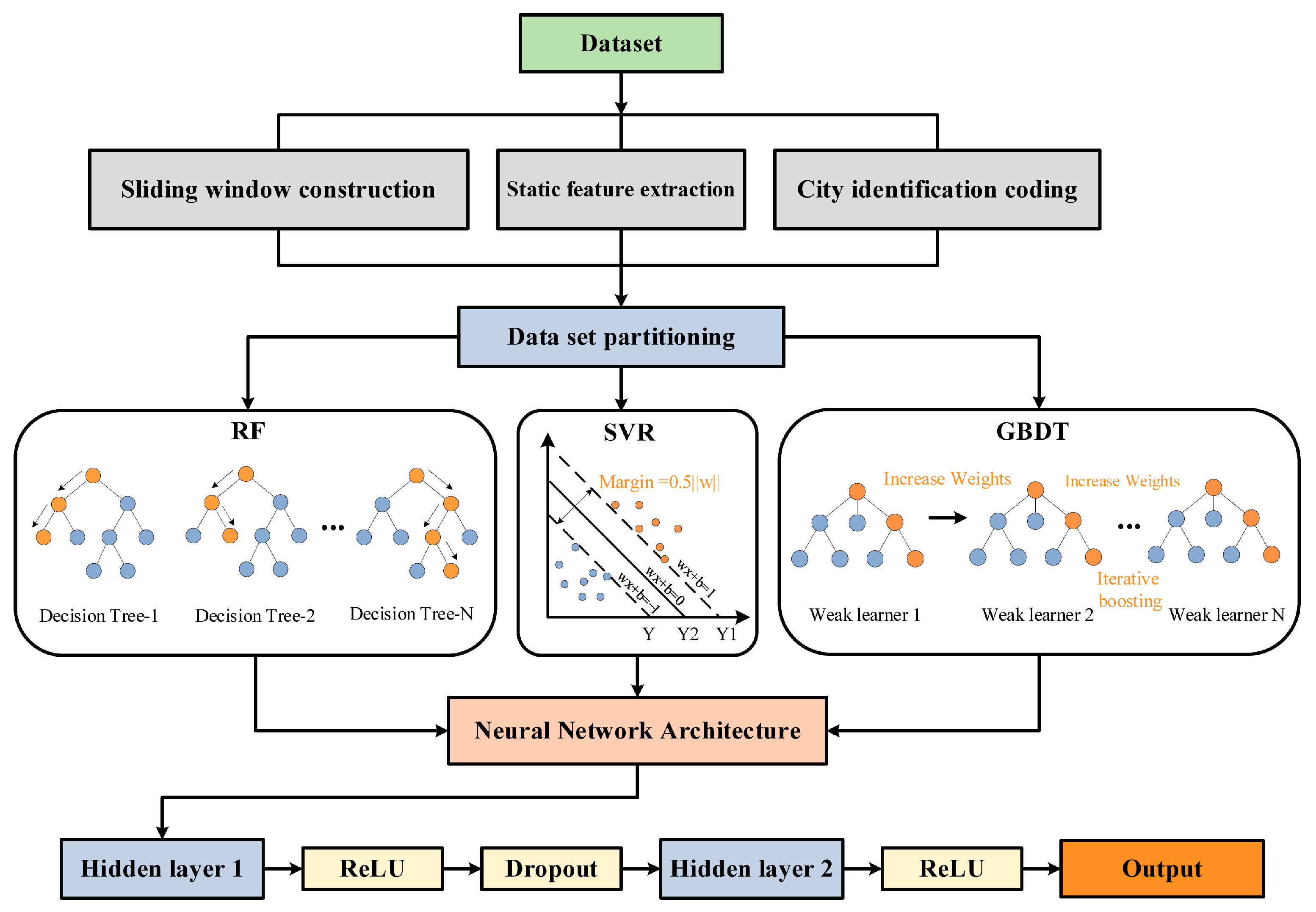
RSG-Net is a two-stage ensemble framework. It combines RF’s strengths in high-dimensional feature interaction and noise robustness with SVR’s specialized capacity for modeling complex nonlinear relationships and GBDT’s gradient-based residual correction mechanism, further enhanced through a shallow neural network to achieve superior predictive performance. The core principle of RSG-Net relies on a base-model feature capture and nonlinear fusion architecture, involving two processing levels: the first-level base model layer comprises RF, SVR, and GBDT in parallel, with each model extracting heterogeneous feature representations; the second-level fusion layer takes the prediction values of the first-level models as inputs and employs a shallow neural network (equipped with dropout regularization, ReLU activation function, and Adam optimizer) to learn the nonlinear relationships among the prediction results, ultimately outputting the fused prediction values.
In feature engineering, the model employs a sliding window to extract dynamic temporal features, static metrics to characterize long-term trends, and urban-specific one-hot encoding to quantify spatial heterogeneity. Subsequently, overfitting is mitigated through the synergistic optimization of first-level model parameters and second-level network dropout regularization, while GPU acceleration is adopted to enhance training efficiency. Furthermore, the model integrates the SHAP (Shapley Additive Explanations) interpreter to quantitatively evaluate the magnitudes of feature importance, thereby enabling interpretable modeling of the relationships between UF and ACE. The architectural flowchart of RSG-Net is presented in Figure 2.
In terms of model parameter configuration, the hyperparameters of the base-level models were not tuned via cross-validation but were instead determined based on insights from the multiple experimental trials to achieve a balance between model accuracy and computational efficiency. The meta-learner comprises a three-layer fully connected neural network with 16, 8, and 1 neurons in successive layers. The hidden layers adopt the ReLU activation function, while the output layer employs a linear activation. A dropout rate of 0.2 is applied after the first layer to mitigate overfitting. The model was trained for 500 epochs using the Adam optimizer with a learning rate of 0.005. During training, the meta-learner adaptively learns the weighting relationships among RF, SVR, and GBDT, thereby enabling data-driven dynamic weighted integration.

2.3.4. Evaluation of Model Accuracy

Model performance evaluation uses comprehensive multi-dimensional indicators, including the coefficient of determination (R2), root mean square error (RMSE), residual prediction deviation (RPD), and percentage bias (PBIAS), to fully characterize both the consistency between predicted values and actual measured values and the features of systematic deviation. R2 denotes the model’s capacity to account for the variation in explanatory variables, with its value ranging from 0 to 1. The nearer this value is to 1, the stronger the model’s goodness of fit. RMSE quantifies the dispersion of prediction errors, with smaller values indicating higher prediction accuracy. RPD assesses the stability of the model by comparing the standard deviation with the prediction error. When RPD > 3, the predictive performance is excellent. When 2 < RPD ≤ 3, it is considered good. When 1.4 < RPD ≤ 2, it is usable but requires careful interpretation. When RPD ≤ 1.4, the model is considered unreliable. PBIAS reveals the sign of systematic deviation. When |PBIAS| < 10%, the deviation is considered acceptable. The standardized expressions of the calculation formulas are as follows [41]:
R 2 = 1 i = 1 n ( y t r u e y p r e d ) 2 i = 1 n y t r u e y ¯ t r u e 2
R M S E = 1 n i = 1 n ( y t r u e y p r e d ) 2
R P D = 1 n 1 i = 1 n y t r u e y ¯ t r u e 2 R M S E
P B I A S = 100 % × i = 1 n ( y p r e d y t r u e ) i = 1 n y t r u e
where y p r e d represents the predicted CO2 emission, y t r u e denotes the measured CO2 emission, y ¯ t r u e signifies the average CO2 emission, and n is the number of samples.

2.3.5. Model Building

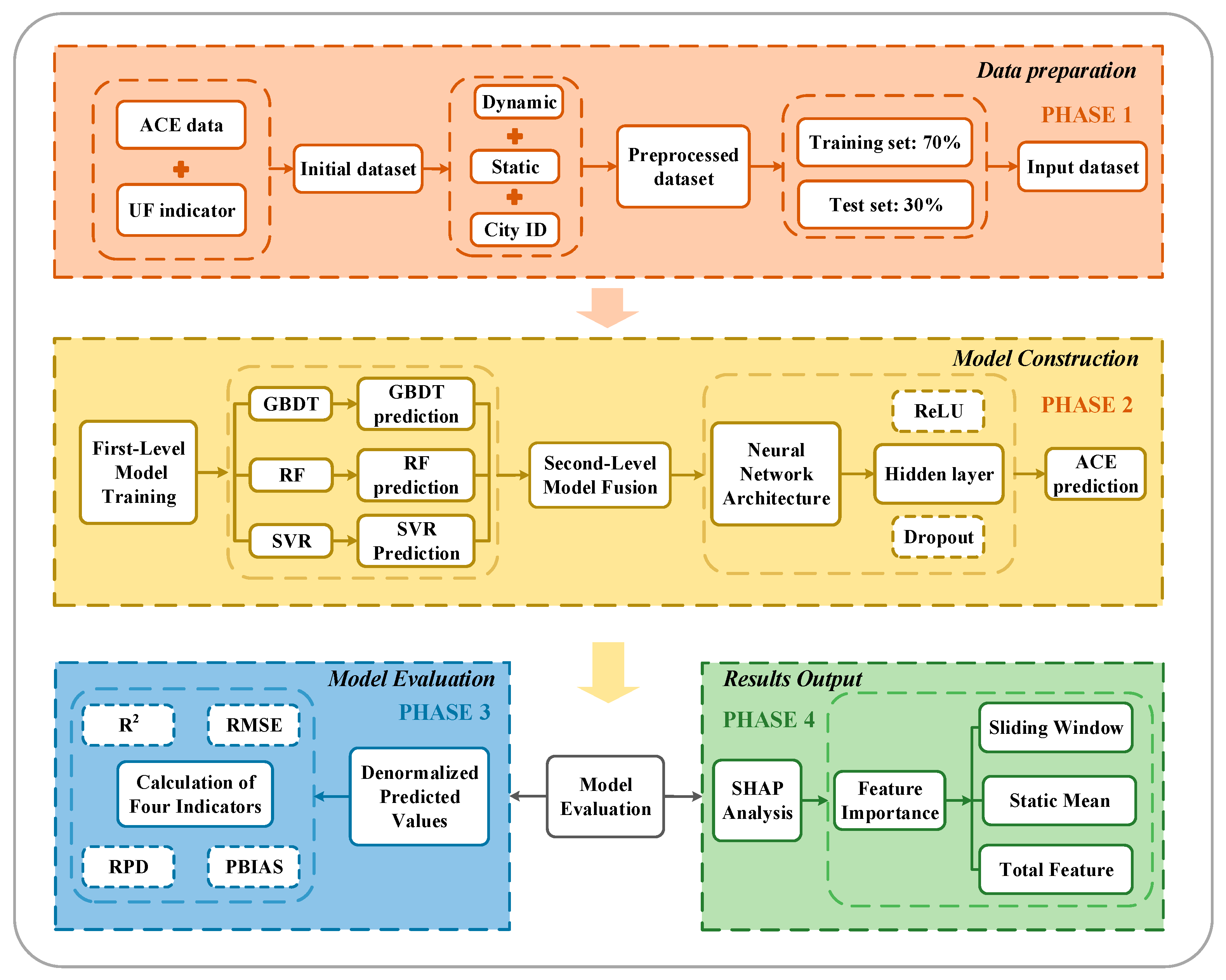
To quantify UF characteristics, this study used city administrative boundaries at the prefecture level to define analysis units, selected 107 UF indicators as independent variables, and constructed a raw dataset with the annual total ACE as the dependent variable. The dataset was processed through three spatiotemporal feature engineering steps, namely sliding window construction, static feature extraction, and urban identification encoding, resulting in 214 valid samples. The training and test sets were randomly split at a 7:3 ratio, with model performance evaluated using R2, RMSE, RPD, and PBIAS.
The model was trained using pooled data covering the years 2002–2022. We employ a sliding-window approach to capture short-term temporal patterns in UF: city samples are ordered chronologically, and indicators from three consecutive periods (window_size = 3) are used as inputs to predict ACE in the subsequent period. The candidate feature set contains 14 UF indicators (F = 14). Static features are constructed at the city level by taking column-wise means over all years for numeric variables, yielding a 14-dimensional static vector that represents long-term stability. During training, the dynamic segment (3F), the static vector (F), and the one-hot encoding of city ID (length C) are concatenated column-wise to form the final input (dimension 56 + C); this city-identity encoding enables the model to explicitly distinguish city-specific fixed effects and spatial heterogeneity. To ensure commensurate scales and numerical stability, both inputs and targets are normalized to [0, 1] using MinMaxScaler. Ultimately, these three feature blocks are concatenated to construct the training samples for subsequent model fitting and prediction. The overall data composition and model workflow are provided in Table 3 and Figure 3.

3. Results

3.1. ACE Inversion Analysis

3.1.1. CO2 Prediction Model

Table 4 presents the regression prediction model developed in this study, which integrates the total nighttime light (TDN) values with the statistical data of ACE, providing a robust framework for quantifying the spatial correspondence between light intensity and carbon output. F denotes the model’s overall significance statistic, while p represents the corresponding significance probability. High F and low p values (p < 0.0001) confirm the model’s statistical significance and overall reliability. The results indicate that the regression model effectively captures the spatial relationship between nighttime luminosity and ACE. Among these datasets, nighttime luminosity demonstrated a statistically significant association with CO2 emissions, consistent with established research findings [42,43]. The R2 values for all provinces and municipalities exceed 0.870, with F values surpassing 77.0. This indicates that it is feasible to extract the TDN values of various cities based on nightlight data and apply the established regression prediction model to estimate the ACE of YREB cities from 2002 to 2022.

3.1.2. ACE Spatio-Temporal Evolution Analysis

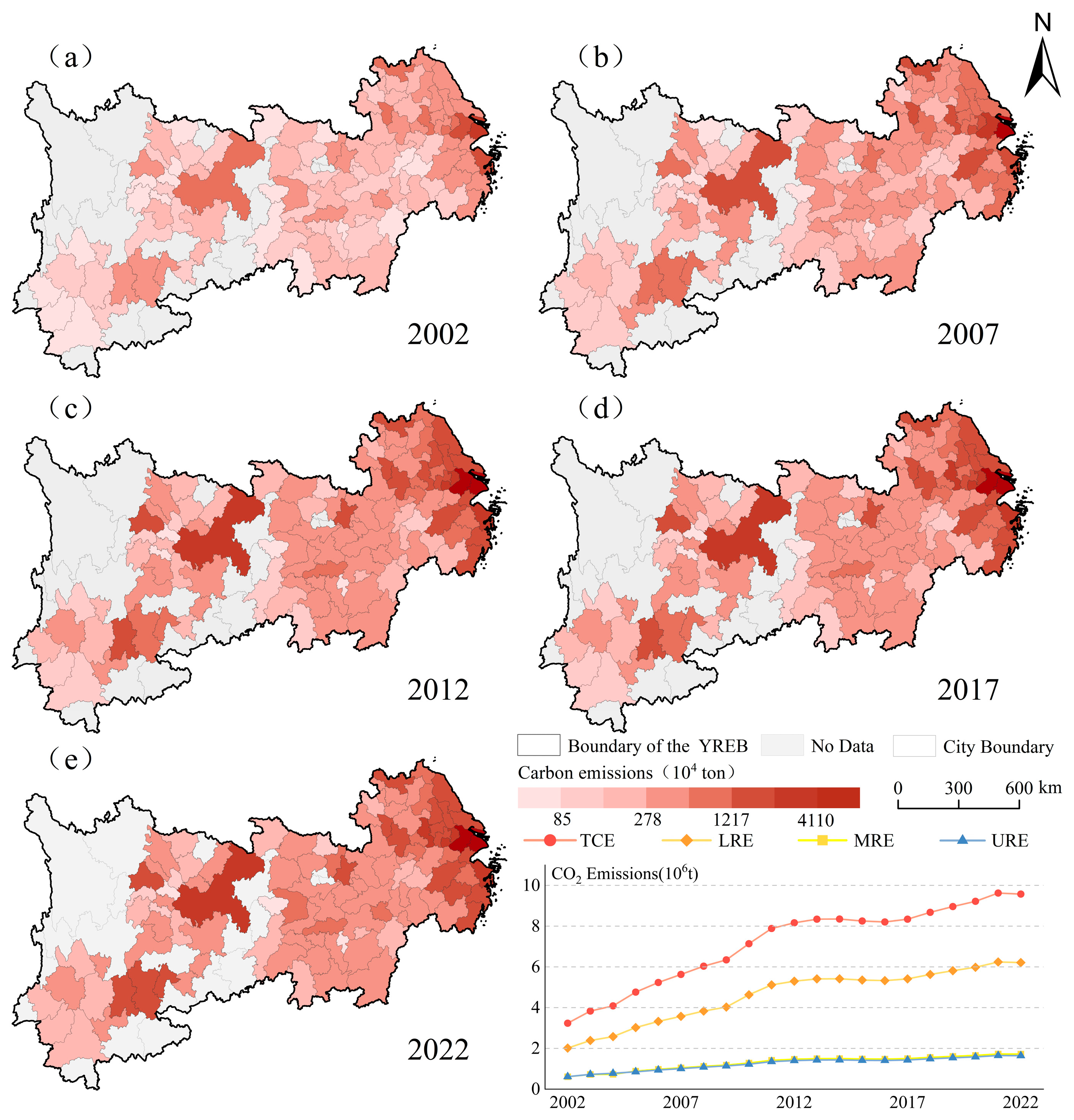
Based on the provincial carbon emission prediction model, municipal ACE can be derived. As shown in Table 5 and Figure 4, ACE in the YREB has continued to increase, with Total CO2 Emissions (TCE) rising from 323.64 Mt to 957.42 Mt. During this period, the growth rate exhibited a phased pattern of rapid growth, slowdown, and recovery. In 2022, Lownstream Regions (LRE) reached 621.16 Mt, accounting for 64.9% of the total; Upstream Regions (URE) increased from 60.88 Mt to 171.88 Mt, and Midstream Regions (MRE) rose from 61.19 Mt to 164.38 Mt. The growth rates of the latter two regions were similar and lower than that of LRE. Spatially, the Yangtze River Delta evolved from a single-pole agglomeration in 2002 to the diffusion of secondary poles in Wuhan and the Chengdu–Chongqing region from 2007 to 2017, and finally to a three-pillar collaborative structure in 2022, consisting of the downstream Yangtze River Delta, the midstream urban agglomeration, and the upstream Chengdu-Chongqing region.

3.2. UF Indicators Analysis

3.2.1. UF Landscape Pattern Index Analysis

Given the staged nature of built-up area expansion, this study adopts five-year intervals and uses nighttime light and socioeconomic data to delineate urban built-up areas and compute their landscape metrics. We then analyze the evolution of the internal structure of YREB cities along three dimensions: sprawl, morphological complexity, and aggregation. Figure 5 illustrates the spatial evolution of built-up areas in representative YREB cities from 2002 to 2022. These trends align with the region’s overall expansion pattern, exhibiting a multi-centered, networked development structure. The total area of built-up areas expanded from 7230.11 km2 in 2002 to 20,724.91 km2 in 2022, with an average annual growth rate of 5.53%. Among these regions, the largest built-up area expanded from 549.58 km2 to 1640.80 km2, whereas the smallest grew from 2.6 km2 to 3.24 km2; meanwhile, the mean value of CA increased from 83.72 km2 to 252.11 km2.
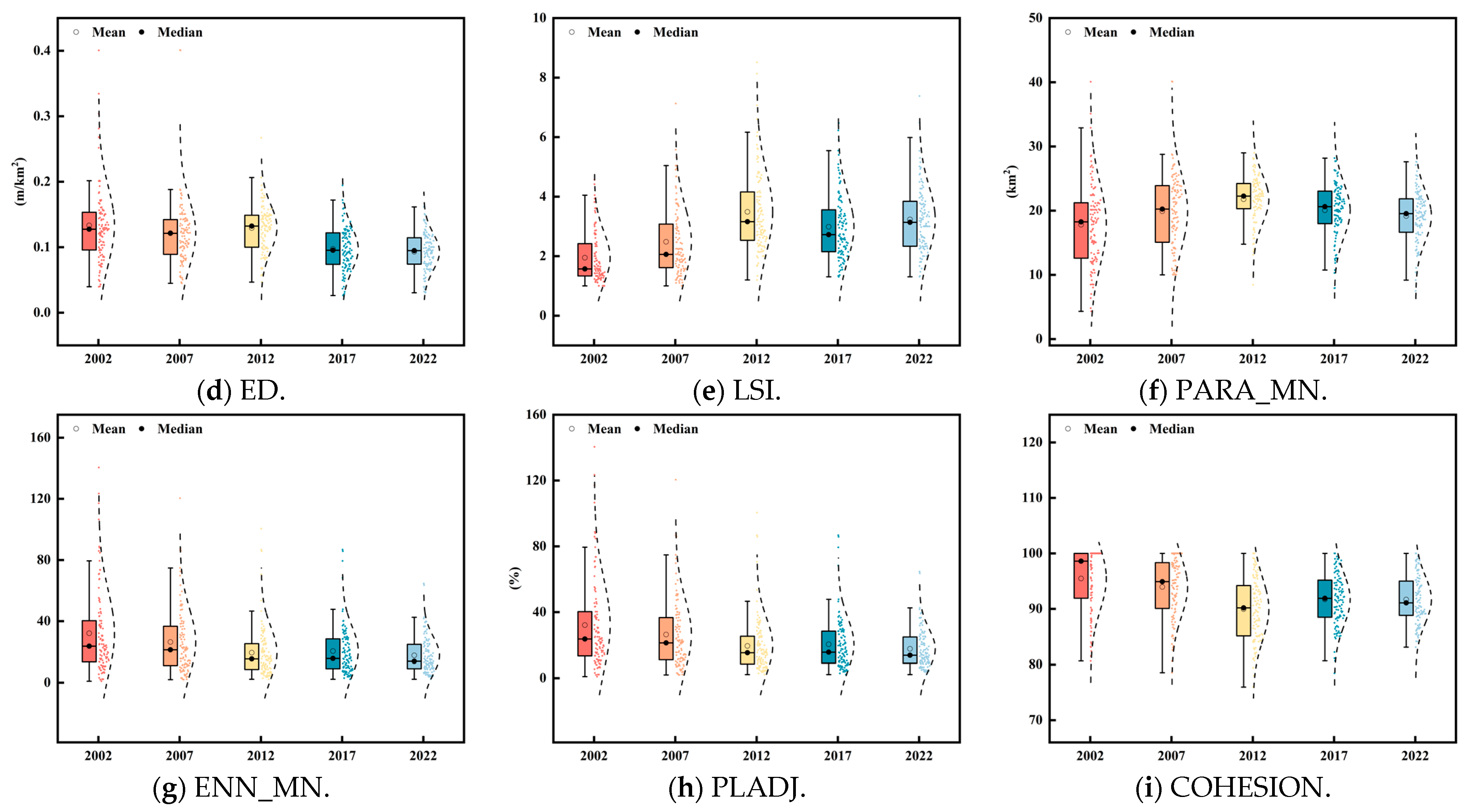
Based on Table A1 and Figure 6, in terms of urban sprawl, the median NP peaked at 35 in 2012 and subsequently declined to 25. The median ED decreased by 41.7%, and the ENN_MN boxplot exhibited a significant downward trend—both indicators suggest the urban development model is shifting from decentralized expansion to intensive integration, an observation that aligns with the findings presented by Wang et al. [44]. In terms of morphological complexity, the mean PD decreased from 0.08 to 0.04, with the box in the figure showing a sustained downward shift; the median LSI increased by 80.9%, with the maximum value rising from 4.6 to 7.4 while the minimum remained stable; and PARA_MN fluctuated between 18 and 22, with its dispersion reducing after 2012. In terms of functional concentration, the average LPI decreased by 22.59%, whereas PLADJ increased from 68% to 78%, and the box position shifted upward over time. This spatial pattern likely reflects the transition of urban morphology from monocentric sprawl to polycentric network development [45], and further confirms the pattern that cohesion within newly developed areas remains relatively weak during urban expansion [46].

3.2.2. UF Characteristic Element Analysis

Five representative characteristic element indicators were selected to perform a further analysis of UF. The following is a comprehensive analysis of each secondary indicator based on Table A2 and Figure 7.
First, in terms of population size and road transportation, both PopDen and RD exhibit a spatial sprawl trend: the maximum PopDen increased consistently from 2585.49 persons/km2 in 2002 to 4729.46 persons/km2 in 2022, representing an 83% increase over two decades, and high-PopDen areas shifted from the central urban districts of major cities in 2002 to a distinct core-periphery zonal pattern and riverine population agglomeration belt by 2022; the mean RD doubled to 1.48 km/km2, consistent with the spatial evolution of roads from scattered distribution to river-basin zonal agglomeration. In the urban land-use dimension, the mean CLC increased from 0.06 to 0.12, with its maximum rising to 1.21, and construction land shifted from discrete, patchy distribution in the early construction stage to contiguous expansion during the YREB urbanization process; between 2002 and 2022, high-value DI areas remained concentrated in the Yangtze River Delta urban agglomeration, while the mean BLR stabilized at approximately 0.97, accompanied by reduced standard deviation and a declining proportion of high-value areas in the distribution map.
In terms of the natural environment, the mean NDVI ranged between 0.73 and 0.75, with high-value areas consistently distributed in the mountainous regions of southwest China. Meanwhile, the overall change in WAR was minimal, though a localized contraction of urban water bodies was observable. The economic and industrial dimensions showed the most significant changes: the mean GDP increased from 45.03 billion to 495.12 billion yuan, a more than tenfold growth that corresponded to its spatial expansion from scattered points to contiguous areas. Additionally, the industrial structure underwent continuous optimization—SI exhibited a pattern of initial increase followed by a decrease, with its peak declining from 51.26% to 44.82%, while TI increased steadily to 48.02%. From a regional perspective, a differentiated distribution pattern is evident, with the secondary industry gradually shifting inland and the tertiary industry clustering along the river.

3.3. Correlation Analysis Between ACE and UF Indicators

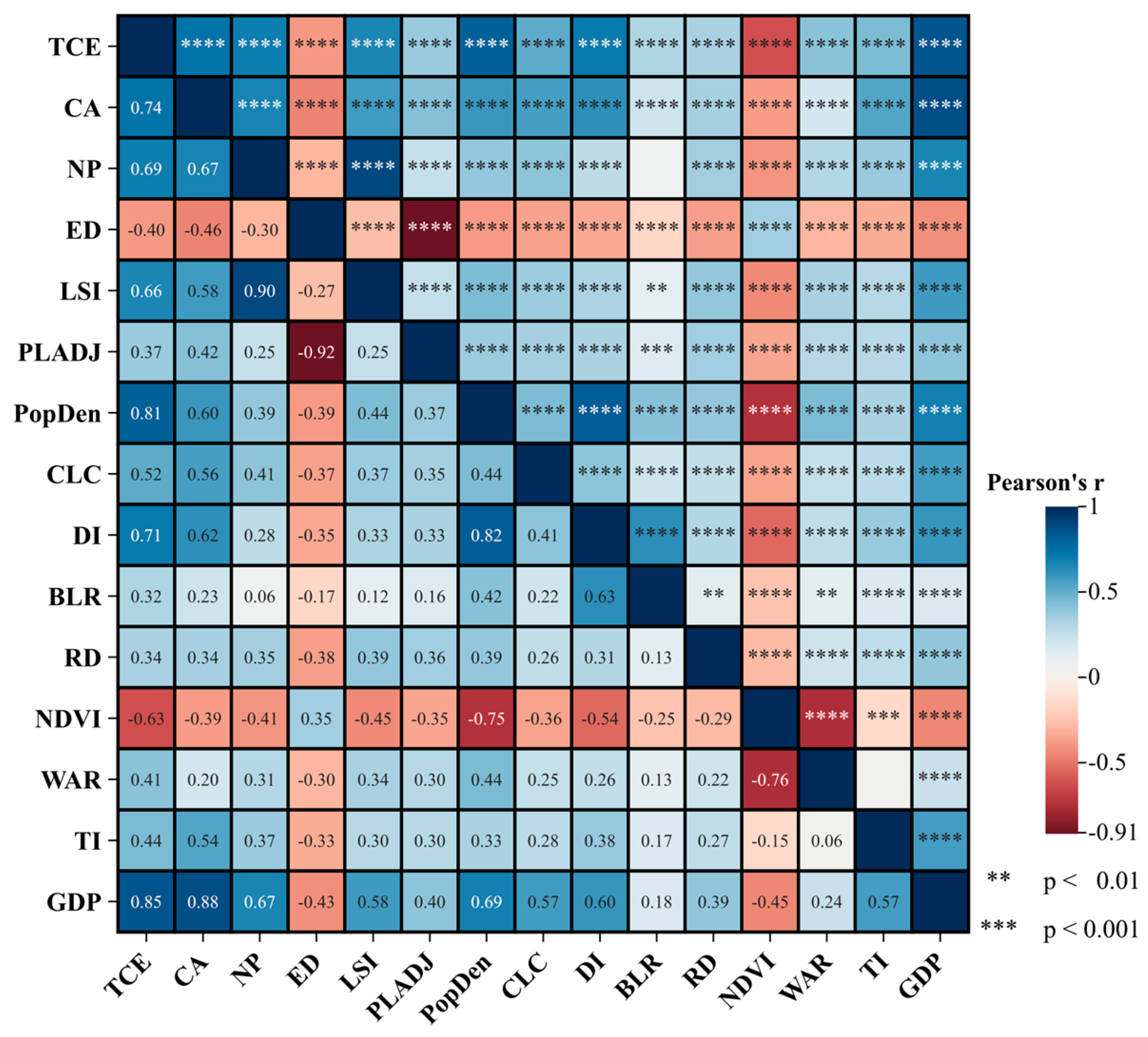
This study employed Pearson’s correlation coefficient approach to analyze the correlation between ACE and 20 UF indicators across 107 cities. As shown in Table 6 and Figure 8, after calculating the correlation coefficients between various UF indicators and ACE, it was found that TCE in this region is positively correlated with parameters such as CA, NP, LSI, PARA_MN, PLADJ, COHESION, PopDen, RD, GDP, TI, CLC, DI, BLR, and WAR. This indicates that as these UF indicators increase during urban development, the ACE will increase accordingly. TCE shows a negative correlation with indicators such as PD, LPI, ED, ENN_MN, NDVI, and SI, indicating that as the values of these UF indicators increase, ACE decreases.
Among the influencing factors, GDP, PopDen, and CA are most strongly correlated with ACE, with Pearson correlation coefficients of 0.855, 0.793, and 0.740, respectively, all of which are higher than those of other indicators. The correlations of RD, TI, DI, NP, LSI, and other factors with TCE were 0.320, 0.450, 0.706, 0.697, 0.662, and 0.389, respectively. In contrast, a negative correlation exists between NDVI and ED, with respective correlation coefficients of −0.609 and −0.389. Accordingly, six indicators with weak correlations with ACE (PD, LPI, PARA_MN, ENN_MN, COHESION, and SI) were excluded. In the subsequent modeling analysis, 14 UF indicators that exhibited significant correlations with ACE were selected as input variables. Figure 8 presents the correlation heatmap between TCE and these highly correlated UF indicators.

3.4. Model Analysis

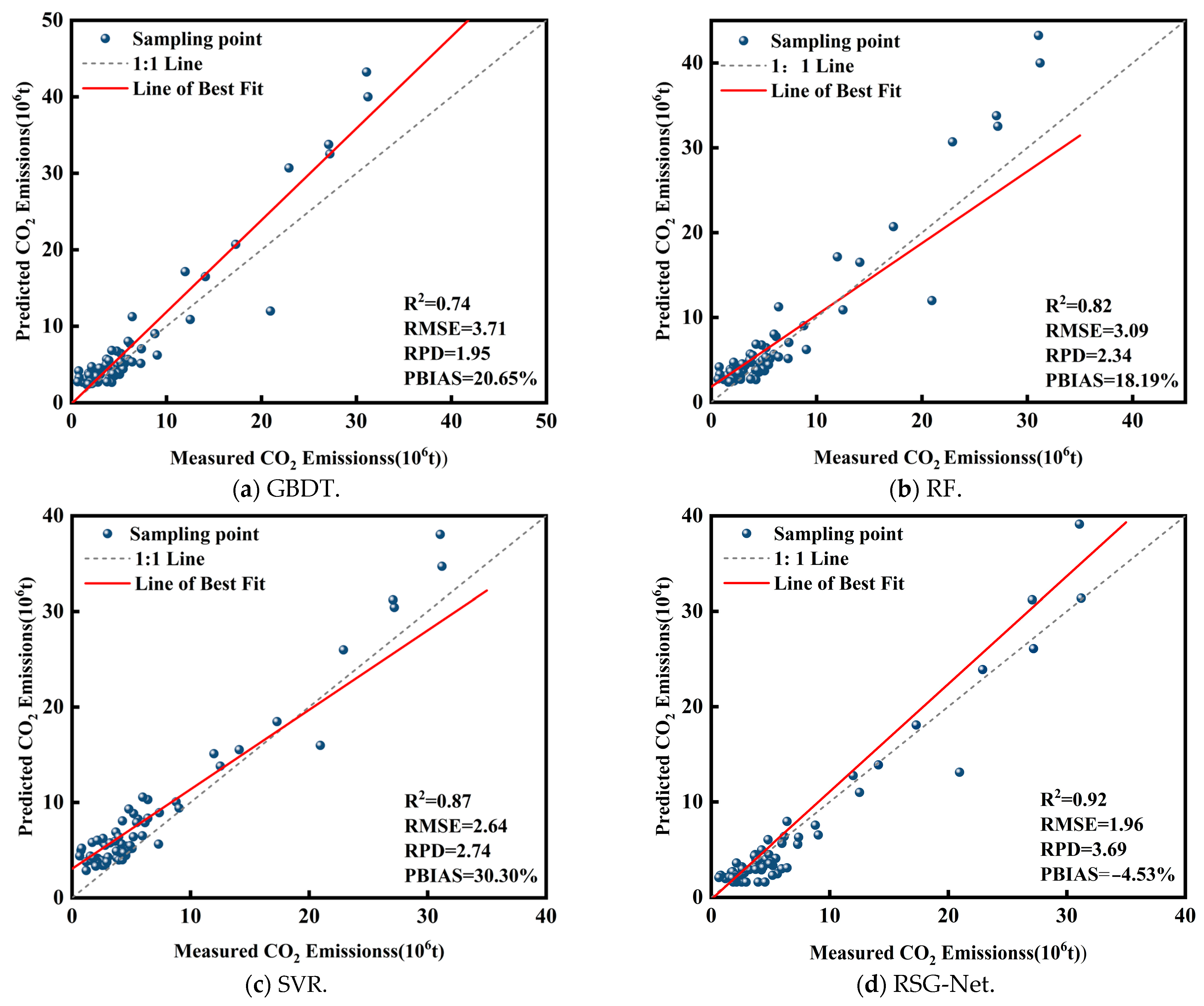
Plot the predicted carbon dioxide emissions from the test set on a scatter-regression chart, predicted by the measured data. As illustrated in Figure 9, the predictive performance of four machine learning models can be compared: GBDT, RF, SVR, and RSG-Net. The RPD of all four models is greater than 1.9, which confirms their predictive capacity. Among them, the predictive performance of the GBDT model is relatively average, with obvious scatter and dispersion characteristics. Its R2 and RPD values are relatively low, with an RMSE of 3.71 and a PBIAS showing overestimation. The RF model shows improvement compared to the GBDT model, with R2 improved to 0.82 and RMSE reduced to 3.09 Mt. In the scatter plot of the prediction of the test set, the concentration in the median area is improved, but outliers still exist in the high-value area. The R2 value of the SVR model reached 0.87, with an RMSE of 2.75 Mt. Outliers were significantly reduced, and the deviation distribution tended to be balanced. The comprehensive index of RSG-Net significantly outperforms other models. The test set R2 reaches 0.93, RMSE is reduced to 1.96 Mt, RPD jumps to 3.68, and PBIAS is 4.53%. Furthermore, the prediction points are closely distributed near the 1:1 line, and the prediction of the full range of values is highly consistent, achieving the best prediction results. Overall, the integrated model RSG-Net improves prediction accuracy and stability by efficiently combining the advantages of each basic model.

4. Discussion

4.1. Model Performance

This study predicted anthropogenic carbon emissions using GBDT, RF, SVR, and RSG-Net ensemble models, with the RSG-Net demonstrating the best performance. By comparing the four models, it was found that the RSG-Net prediction accuracy significantly surpassed that of the base models. It effectively compensates for the limitations of a single algorithm in handling the complex relationship between UF and ACE. On the test set, the RSG-Net model achieved an R2 of 0.93, an RPD of 3.68, and a PBIAS of 4.53%. These results signify substantial improvements over the base models: the R2 value was 6.90%, 13.41%, and 25.68% higher than that of the SVR, RF, and GBDT models, respectively; the RPD value was 33.82%, 57.26%, and 88.72% higher, respectively; and the RMSE was reduced by 25.76%, 36.57%, and 47.17%, respectively. Notably, it achieved a PBIAS of just 4.53%, equivalent to merely 15.0%, 24.9%, and 21.9% of the corresponding bias magnitudes of the base models.
The RSG-Net ensemble model systematically integrates CO2 data, socio-economic panel data, and other multi-source information via its heterogeneous data compatibility mechanism. Meanwhile, by tapping into the multi-source feature extraction capabilities of base learners, the model accurately captures ACE’s temporal evolution patterns and UF features across multiple scales. However, for individual models, GBDT is sensitive to outliers and tends to overfit noisy data, thereby weakening its generalization performance, which is consistent with the findings of Manley et al. [47]. RF, owing to its bagging-based independent sampling mechanism, has limited ability to capture dynamic dependencies in time series, showing constraints when dealing with data exhibiting strong temporal correlations [48]. SVR exhibits limited accuracy without systematic optimization, as its performance depends heavily on the kernel function and hyperparameter configuration, and excessive reliance on empirical tuning often results in instability [49].
To address these issues, RSG-Net adopts a hybrid architecture that integrates base-model ensembles with meta-learning, in which a shallow neural network serves as the meta-learner. By adaptively optimizing the dynamic weight allocation among base models through nonlinear transformation, it overcomes the limitations of single models. As a result, the ensemble model yields a markedly higher R2 in carbon-emission prediction, consistent with Hu et al. [50], confirming the advantage of ensemble learning in predictive performance. Moreover, the proposed model enhances prediction accuracy while mitigating overfitting, aligning with the findings of Yan et al. [22], who reported greater robustness of ensemble models in long-term carbon-intensity forecasting.

4.2. The Importance of Indicators

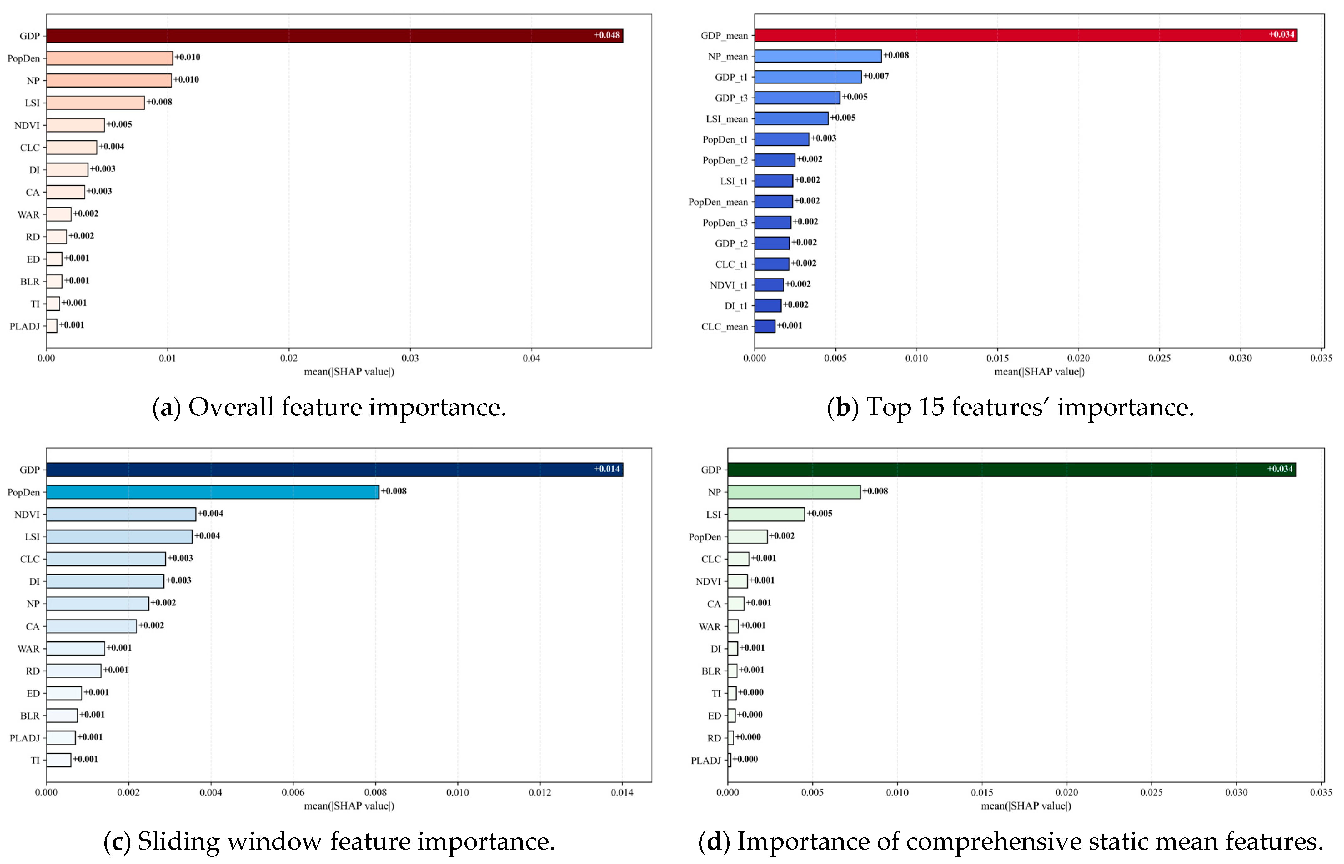
Based on the SHAP analysis of the RSG-Net model, the major driving factors of anthropogenic carbon emissions across 107 cities in the YREB were identified and ranked by importance. The overall and category-specific feature importance results are illustrated in Figure 10. GDP consistently dominated all features, showing a strong positive correlation with TCE and indicating that economic expansion directly promotes carbon growth through industrial and energy activities, consistent with Tang et al. [51].
Landscape fragmentation and morphological complexity, represented by NP and LSI, significantly increased carbon emissions, aligning with Patle and Ghuge [52], who reported that land fragmentation and urban form complexity intensify environmental pressures. As fragmentation deepens, dispersed economic activities and expanded infrastructure demand lead to higher CO2 emissions. Population density and the expansion of road networks jointly regulate the ACE–UF relationship. Over the past two decades, PopDen developed a core–periphery pattern along river corridors, where concentrated energy use and commuting activity increased emissions, consistent with Wang and Zeng [53].
This study also found a significant negative correlation between NDVI and CO2 emissions, indicating that higher vegetation coverage effectively mitigates urban carbon emissions. Higher NDVI values reflect better ecological conditions and stronger carbon sequestration capacity, thereby exerting a notable inhibitory effect on emissions [54]. In addition, CLC changes represent the process of land-use intensification, shifting from fragmented to contiguous patterns. This trend enhances energy efficiency through shared infrastructure and spatial integration, thereby reducing CO2 emissions. Zhang et al. similarly found that higher land-use compactness contributes to effective emission reduction [55], indicating that land compactness plays a significant role in influencing CO2 emissions.

4.3. Carbon Reduction Pathways

Given the substantial disparities in development levels among cities in the YREB, formulating city-specific emission reduction pathways is particularly critical. Based on the preceding empirical analysis, the importance ranking of UF factors indicates that economic scale, population density, spatial agglomeration and complexity, the proportion of blue–green space, and land development patterns all exert significant influences on anthropogenic carbon emissions. Accordingly, four targeted mitigation strategies are proposed, focusing on optimizing the economic structure, adjusting the spatial layout, enhancing ecological space, and guiding land-use patterns.
First, efforts should be made to vigorously develop a green and low-carbon economy. Promoting low-carbon transformation requires differentiated regulation of industrial structures and spatial population layouts. Tang et al. emphasized that the driving mechanisms of carbon emissions vary considerably across cities at different development stages [51]; therefore, mitigation policies should be tailored to local conditions.
Second, unregulated urban sprawl should be curbed. Compact spatial structures can shorten commuting distances, improve land-use efficiency, and reduce transportation energy consumption [53]. Within the YREB, large cities such as Shanghai and Chongqing should delineate strict development boundaries and promote high-density renewal supported by integrated transport systems. Medium-sized cities like Wuhan and Changsha should foster clustered, transit-oriented growth to strengthen the job–housing balance, while small cities in the upper reaches should prioritize land consolidation and the revitalization of built-up areas in accordance with ecological redline policies.
Third, expanding blue–green spaces is essential for strengthening regional carbon sinks. Within the YREB, wetland and coastal restoration in the lower reaches can enhance carbon sequestration and flood resilience. In the middle reaches, improving river–lake connectivity and ecological corridors can facilitate carbon storage and ecosystem regulation, while soil conservation and reforestation in the upper reaches further reduce carbon emissions and reinforce the basin’s ecological security.
Finally, land development patterns should be scientifically guided. Enhancing functional mix and spatial accessibility can optimize energy allocation and reduce consumption [56]. In the YREB, the lower-reach city clusters, such as the Yangtze River Delta, should promote integrated spatial renewal and intensive land-use. The middle-reach clusters, including Wuhan and Changsha–Zhuzhou–Xiangtan, should coordinate urban expansion with ecological protection, whereas the upper-reach Chengdu–Chongqing cluster should prioritize urban regeneration and land consolidation to establish a “low concentration–high efficiency” model for low-carbon development.

5. Conclusions

This study explores the relationship between urban form and anthropogenic carbon emissions in the YREB during 2002–2022. Using night light remote sensing data, the ODIAC dataset, and other auxiliary sources, a novel RSG-Net ensemble model was constructed to reveal the impact of UF on ACE, and targeted carbon reduction pathways are further proposed. The main findings are as follows.
(1)
From 2002 to 2022, the TCE of the YREB increased from 323.64 Mt to 957.42 Mt (Table 5), with its growth rate exhibiting a pattern of rapid growth, slowdown, and recovery (Figure 4). Spatially, the distribution pattern evolved from a unipolar agglomeration centered on the Yangtze River Delta in 2002, progressed through the diffusion of secondary growth poles in the Wuhan Metropolitan Area and Chengdu-Chongqing Urban Agglomeration during 2007–2017, and finally transformed into a new multipolar synergistic spatial model featuring watershed-wide coordination by 2022.
(2)
The RSG-Net ensemble model outperforms individual base models in ACE prediction, achieving an R2 of 0.93, an RPD of 3.69, an RMSE of 1.96 Mt, and a PBIAS of 4.53%. These results indicate that the two-stage hybrid architecture effectively mitigates the limitations of GBDT, RF, and SVR, such as sensitivity to outliers, weak temporal dependency capture, and limited accuracy without optimization. By integrating the complementary strengths of the base learners, RSG-Net significantly enhances prediction stability and accuracy, confirming the effectiveness of combining ensemble learning with meta-learning in carbon emission modeling.
(3)
By combining Pearson correlation and SHAP feature importance analysis, a significant correlation between UF and ACE is confirmed: ACE is positively correlated with CA, NP, LSI, PopDen, GDP, CLC, and WAR, and negatively correlated with PD, LPI, ED, ENN_MN, NDVI, and SI. The key UF factors, ranked by importance, are GDP, PopDen, NP, LSI, NDVI, and CLC. Based on their mechanism, implementing measures such as promoting low-carbon economic transformation, enhancing urban spatial agglomeration, and strengthening ecological carbon sequestration can effectively reduce ACE values and facilitate precise urban carbon reduction.
This study developed the RSG-Net ensemble model and integrated the SHAP method. Through a two-stage hybrid architecture, the model achieved high-accuracy ACE prediction, clarified the importance ranking of key UF factors, and provided a scientific basis for urban carbon reduction pathways. However, the study has limitations: the current city-level analysis does not fully consider small-scale spatial interactions, factor synergy mechanisms, or threshold effects. Future research should extend the analysis to finer spatial scales and conduct comparative assessments with other ensemble and deep learning models to further optimize the RSG-Net, enhance its local pattern recognition capability, and develop more generalizable guidelines for low-carbon urban planning.

Author Contributions

Conceptualization and writing—original draft preparation, J.L. and Q.W.; methodology, Q.G. and W.L.; supervision, Y.S. and S.F.; data curation, J.L. and Z.D.; writing—review and editing, J.L. and B.P.; funding acquisition, B.P. All authors have read and agreed to the published version of the manuscript.

Funding

The author gratefully acknowledges the financial support from the National Natural Science Foundation of China (42277075), Key Science and Technology Projects under the Science and Technology Innovation Platform (202305a12020039), Anhui Natural Science Research Foundation (2208085US14), Anhui Provincial Science and Technology Plan Project for Housing and Urban-Rural Construction (2024-YF055), Natural Science Foundation of colleges and universities in Anhui Province (2023AH050187).

Institutional Review Board Statement

Not applicable.

Informed Consent Statement

Not applicable.

Data Availability Statement

The original contributions presented in the study are included in the article, further inquiries can be directed to the corresponding author.

Conflicts of Interest

The authors declare no conflicts of interest.

Appendix A

Table A1. Statistical analysis of dependent and independent variables (LSPI aspect).
YearSTADVIV
TCE
(104 t)
CA
(km2)
NP
(n)
PD
(%)
LPI
(%)
ED
(m/km2)
LSI
(−)
PARA_MN
(km2)
ENN_MN
(−)
PLADJ
(%)
COHESION
(−)
2002Max2988.04549.5816.000.67100.000.404.5740.07140.4790.11100.00
Min19.632.601.000.0031.780.041.004.300.990.0047.10
Mean302.4767.573.140.0985.120.131.9517.8032.1066.8794.54
Std378.9083.723.150.1018.690.060.876.3427.7114.698.07
2007Max5423.49885.6727.001.01100.000.407.1340.13120.4788.82100.00
Min39.1211.601.000.0123.910.041.0010.001.990.000.00
Mean526.1991.515.020.0779.360.122.4819.9126.3969.7993.09
Std701.54125.984.910.1119.070.051.195.8621.7012.7010.49
2012Max7456.851051.7149.000.22100.000.278.5129.01100.4788.37100.00
Min55.6415.181.000.0123.460.051.208.442.2333.3375.96
Mean763.26127.048.980.0765.360.133.4921.7819.4467.8389.96
Std1034.27167.797.850.0417.300.041.353.7316.948.805.56
2017Max7614.041423.0942.000.14100.000.196.4728.1886.7693.49100.00
Min56.7422.501.000.0033.680.031.317.922.2351.7278.45
Mean779.82164.298.360.0570.410.102.9920.0520.4875.7591.72
Std1056.53209.587.000.0316.450.031.114.1916.058.224.70
2022Max8735.161640.8049.000.11100.000.167.3827.6264.6092.45100.00
Min65.0523.241.000.0032.420.031.317.482.2359.8183.11
Mean894.78193.699.680.0565.890.093.2319.1717.7076.8891.69
Std1212.21252.117.590.0217.010.031.113.9312.146.964.27
Table A2. Statistical analysis of dependent and independent variables (UMC aspect).
YearSTADVIV
TCE
(10−4 t)
PopDen
(Person/km2)
RD
(km/km2)
SI
(%)
TI
(%)
GDP
(Billion Yuan)
NDVI
(−)
WAR
(%)
DI
(−)
BLR
(%)
CLC
(−)
2002Max2988.042585.491.2668.7056.155795.020.820.370.293.320.30
Min19.6356.640.2319.7024.1036.950.490.000.000.100.00
Mean302.47473.390.5043.0236.58454.500.740.050.010.970.05
Std378.90326.610.1910.215.64676.720.050.060.030.290.06
2007Max5423.493119.801.8171.3259.4412,878.680.840.360.382.740.38
Min39.1258.480.2823.7923.9284.820.510.000.000.430.00
Mean526.19485.621.0247.0436.38998.730.760.040.011.030.08
Std701.54375.850.349.846.301536.700.050.050.040.240.08
2012Max7456.853781.762.2475.8662.3321,305.590.840.350.462.910.46
Min55.6458.650.3225.2020.66212.240.450.000.000.010.00
Mean763.26501.481.2151.7435.232172.800.750.050.021.000.08
Std1034.27443.030.398.258.142889.030.070.050.050.270.08
2017Max7614.044034.452.3366.4069.8430,429.260.870.340.301.910.34
Min56.7460.250.3819.4817.71330.030.500.000.000.740.01
Mean779.82519.651.3445.2443.313354.160.770.050.020.980.08
Std1056.53466.460.417.177.964362.240.060.050.030.130.07
2022Max8735.164729.462.634737.0074.1244,653.000.880.310.171.421.21
Min65.0558.100.0012.8135.27592.000.490.000.000.620.01
Mean894.78518.141.5085.1148.464997.470.760.040.020.960.11
Std1212.21519.930.49451.896.856408.030.070.050.020.110.18

References

  1. Cai, B.; Zhang, L. Urban CO2 Emissions in China: Spatial Boundary and Performance Comparison. Energy Policy 2014, 66, 557–567. [Google Scholar] [CrossRef]
  2. Wang, S.; Wang, J.; Fang, C.; Li, S. Estimating the Impacts of Urban Form on CO2 Emission Efficiency in the Pearl River Delta, China. Cities 2019, 85, 117–129. [Google Scholar] [CrossRef]
  3. Xiang, W.; Lan, Y.; Gan, L.; Li, J. How Does New Urbanization Affect Urban Carbon Emissions? Evidence Based on Spatial Spillover Effects and Mechanism Tests. Urban Clim. 2024, 56, 102060. [Google Scholar] [CrossRef]
  4. Liu, Z.; Deng, Z.; Davis, S.J.; Giron, C.; Ciais, P. Monitoring Global Carbon Emissions in 2021. Nat. Rev. Earth Environ. 2022, 3, 217–219. [Google Scholar] [CrossRef]
  5. Wei, L.; Liu, Z. Spatial Heterogeneity of Demographic Structure Effects on Urban Carbon Emissions. Environ. Impact Assess. Rev. 2022, 95, 106790. [Google Scholar] [CrossRef]
  6. Li, J.S.; Zhou, H.W.; Meng, J.; Yang, Q.; Chen, B.; Zhang, Y.Y. Carbon Emissions and Their Drivers for a Typical Urban Economy from Multiple Perspectives: A Case Analysis for Beijing City. Appl. Energy 2018, 226, 1076–1086. [Google Scholar] [CrossRef]
  7. Lei, H.; Zeng, S.; Namaiti, A.; Zeng, J. The Impacts of Road Traffic on Urban Carbon Emissions and the Corresponding Planning Strategies. Land 2023, 12, 800. [Google Scholar] [CrossRef]
  8. Du, L.; Li, X.; Zhao, H.; Ma, W.; Jiang, P. System Dynamic Modeling of Urban Carbon Emissions Based on the Regional National Economy and Social Development Plan: A Case Study of Shanghai City. J. Clean. Prod. 2018, 172, 1501–1513. [Google Scholar] [CrossRef]
  9. Xie, R.; Fang, J.; Liu, C. The Effects of Transportation Infrastructure on Urban Carbon Emissions. Appl. Energy 2017, 196, 199–207. [Google Scholar] [CrossRef]
  10. Beller, E.E.; Kelly, M.; Larsen, L.G. From Savanna to Suburb: Effects of 160 Years of Landscape Change on Carbon Storage in Silicon Valley, California. Landsc. Urban Plan. 2020, 195, 103712. [Google Scholar] [CrossRef]
  11. Feng, Y.; Chen, S.; Tong, X.; Lei, Z.; Gao, C.; Wang, J. Modeling Changes in China’s 2000–2030 Carbon Stock Caused by Land Use Change. J. Clean. Prod. 2020, 252, 119659. [Google Scholar] [CrossRef]
  12. Bereitschaft, B.; Debbage, K. Urban Form, Air Pollution, and CO2 Emissions in Large U.S. Metropolitan Areas. Prof. Geogr. 2013, 65, 612–635. [Google Scholar] [CrossRef]
  13. Shi, F.; Liao, X.; Shen, L.; Meng, C.; Lai, Y. Exploring the Spatiotemporal Impacts of Urban Form on CO2 Emissions: Evidence and Implications from 256 Chinese Cities. Environ. Impact Assess. Rev. 2022, 96, 106850. [Google Scholar] [CrossRef]
  14. Ding, G.; Guo, J.; Pueppke, S.G.; Yi, J.; Ou, M.; Ou, W.; Tao, Y. The Influence of Urban Form Compactness on CO2 Emissions and Its Threshold Effect: Evidence from Cities in China. J. Environ. Manag. 2022, 322, 116032. [Google Scholar] [CrossRef]
  15. Wu, J.; Li, C. Illustrating the Nonlinear Effects of Urban Form Factors on Transportation Carbon Emissions Based on Gradient Boosting Decision Trees. Sci. Total Environ. 2024, 929, 172547. [Google Scholar] [CrossRef]
  16. Li, M.; Zhou, Q.; Yang, Y. Study on the Influence of Urban Factors on Land Surface Temperature in Xi’an Based on Support Vector Machine. Intell. Build. Smart City 2023, 11, 13–15. [Google Scholar] [CrossRef]
  17. Dodangeh, E.; Choubin, B.; Eigdir, A.N.; Nabipour, N.; Panahi, M.; Shamshirband, S.; Mosavi, A. Integrated Machine Learning Methods with Resampling Algorithms for Flood Susceptibility Prediction. Sci. Total Environ. 2020, 705, 135983. [Google Scholar] [CrossRef]
  18. Chaturvedi, V.; De Vries, W.T. Machine Learning Algorithms for Urban Land Use Planning: A Review. Urban Sci. 2021, 5, 68. [Google Scholar] [CrossRef]
  19. Xing, Y.; Song, X.; Li, F.; Li, M.; Guo, Q.; Zhang, L. Ensemble Learning Algorithm Combined with Empirical Models for the Prediction of Urban Air Pollutant Emissions. Environ. Monit. China 2025, 41, 14–23. [Google Scholar] [CrossRef]
  20. Jiang, S.; Tian, S. Stacked Ensemble Learning for Predicting Carbon Emissions Throughout the Life Cycle of Buildings. In Proceedings of the 2025 4th International Conference on Distributed Computing and Electrical Circuits and Electronics (ICDCECE), Ballari, India, 25–26 April 2025; pp. 1–8. [Google Scholar]
  21. Requia, W.J.; Di, Q.; Silvern, R.; Kelly, J.T.; Koutrakis, P.; Mickley, L.J.; Sulprizio, M.P.; Amini, H.; Shi, L.; Schwartz, J. An Ensemble Learning Approach for Estimating High Spatiotemporal Resolution of Ground-Level Ozone in the Contiguous United States. Environ. Sci. Technol. 2020, 54, 11037–11047. [Google Scholar] [CrossRef]
  22. Yan, L.; Wang, L.; Liu, S.; Ding, Y. EnsembleCI: Ensemble Learning for Carbon Intensity Forecasting. In Proceedings of the 16th ACM International Conference on Future and Sustainable Energy Systems, Rotterdam, The Netherlands, 17–20 June 2025; pp. 208–212. [Google Scholar]
  23. Yang, D.; Luan, W.; Qiao, L.; Pratama, M. Modeling and Spatio-Temporal Analysis of City-Level Carbon Emissions Based on Nighttime Light Satellite Imagery. Appl. Energy 2020, 268, 114696. [Google Scholar] [CrossRef]
  24. Wang, L.; Zhang, N.; Deng, H.; Wang, P.; Yang, F.; Qu, J.J.; Zhou, X. Monitoring Urban Carbon Emissions from Energy Consumption over China with DMSP/OLS Nighttime Light Observations. Theor. Appl. Climatol. 2022, 149, 983–992. [Google Scholar] [CrossRef]
  25. Song, M.; Wang, Y.; Han, Y.; Ji, Y. Estimation Model and Spatio-Temporal Analysis of Carbon Emissions from Energy Consumption with NPP-VIIRS-like Nighttime Light Images: A Case Study in the Pearl River Delta Urban Agglomeration of China. Remote Sens. 2024, 16, 3407. [Google Scholar] [CrossRef]
  26. Yang, Y.; Li, H. Monitoring Spatiotemporal Characteristics of Land-Use Carbon Emissions and Their Driving Mechanisms in the Yellow River Delta: A Grid-Scale Analysis. Environ. Res. 2022, 214, 114151. [Google Scholar] [CrossRef]
  27. Chang, P.; Pang, X.; He, X.; Zhu, Y.; Zhou, C. Exploring the Spatial Relationship Between Nighttime Light and Tourism Economy: Evidence from 31 Provinces in China. Sustainability 2022, 14, 7350. [Google Scholar] [CrossRef]
  28. Liu, X.; Yang, X. The Accuracy of Nighttime Light Data to Estimate China’s Provincial Carbon Emissions: A Comparison with Carbon Emissions Allocated by International Carbon Database. Remote Sens. Technol. Appl. 2022, 37, 319–332. [Google Scholar]
  29. Xu, L.; Du, H.; Zhang, X. Driving Forces of Carbon Dioxide Emissions in China’s Cities: An Empirical Analysis Based on the Geodetector Method. J. Clean. Prod. 2021, 287, 125169. [Google Scholar] [CrossRef]
  30. Yang, W.; Yang, P.; Sun, X.; Han, B. Changes of landscape pattern and its impacts on multiple ecosystem services in Beijing. Acta Ecol. Sin. 2022, 42, 6487–6498. [Google Scholar]
  31. Lan, T.; Shao, G.; Xu, Z.; Tang, L.; Dong, H. Considerable Role of Urban Functional Form in Low-Carbon City Development. J. Clean. Prod. 2023, 392, 136256. [Google Scholar] [CrossRef]
  32. He, X.; Guan, D.; Yang, X.; Zhou, L.; Gao, W. Quantifying the Trends and Affecting Factors of CO2 Emissions Under Different Urban Development Patterns: An Econometric Study on the Yangtze River Economic Belt in China. Sustain. Cities Soc. 2024, 107, 105443. [Google Scholar] [CrossRef]
  33. Guan, D.; Shi, Y.; Zhou, L.; Zhu, X.; Zhao, D.; Peng, G.; He, X. Construction and Application of Carbon Emissions Estimation Model for China Based on Gradient Boosting Algorithm. Remote Sens. 2025, 17, 2383. [Google Scholar] [CrossRef]
  34. Friedman, J.H. Greedy Function Approximation: A Gradient Boosting Machine. Ann. Stat. 2001, 29, 1189–1232. [Google Scholar] [CrossRef]
  35. Sun, Z.; Wang, G.; Li, P.; Wang, H.; Zhang, M.; Liang, X. An Improved Random Forest Based on the Classification Accuracy and Correlation Measurement of Decision Trees. Expert. Syst. Appl. 2024, 237, 121549. [Google Scholar] [CrossRef]
  36. Tang, Z.; Mei, Z.; Liu, W.; Xia, Y. Identification of the Key Factors Affecting Chinese Carbon Intensity and Their Historical Trends Using Random Forest Algorithm. J. Geogr. Sci. 2020, 30, 743–756. [Google Scholar] [CrossRef]
  37. Breiman, L. Random Forests. Mach. Learn. 2001, 45, 5–32. [Google Scholar] [CrossRef]
  38. Smola, A.J.; Schölkopf, B. A Tutorial on Support Vector Regression. Stat. Comput. 2004, 14, 199–222. [Google Scholar] [CrossRef]
  39. Hao, P.Y. Shrinking the Tube: A New Support Vector Regression Algorithm with Parametric Insensitive Model. In Proceedings of the 2007 International Conference on Machine Learning and Cybernetics, Hong Kong, China, 19–22 August 2007; pp. 1871–1874. [Google Scholar]
  40. Song, X.; Zhang, X.; Sun, H.; Lin, S. Modelling of the fore-and-aft in-line seat transmissibility using the support vector regression with hyperparameter optimization algorithms. J. Vib. Eng. 2025, 8. [Google Scholar] [CrossRef]
  41. Pan, B.; Liu, W.; Diao, Z.; Gao, Q.; Huang, L.; Feng, S.; Du, J.; Wang, Q.; Li, J.; Cheng, J. Assessment of a Hyperspectral Remote Sensing Model Performance for Particulate Phosphorus in Optically Shallow Lake Water. J. Spectrosc. 2025, 2025, 9683030. [Google Scholar] [CrossRef]
  42. Li, H.; Long, M.; Li, G. Spatial-temporal dynamics of carbon dioxide emissions in China based on DMSP/OLS nighttime stable light data. China Environ. Sci. 2018, 38, 2777–2784. [Google Scholar] [CrossRef]
  43. Meng, L.; Graus, W.; Worrell, E.; Huang, B. Estimating CO2 (Carbon Dioxide) Emissions at Urban Scales by DMSP/OLS (Defense Meteorological Satellite Program’s Operational Linescan System) Nighttime Light Imagery: Methodological Challenges and a Case Study for China. Energy 2014, 71, 468–478. [Google Scholar] [CrossRef]
  44. Wang, Y.; Fan, H.; Wang, H.; Che, Y.; Wang, J.; Liao, Y.; Lv, S. High-Carbon Expansion or Low-Carbon Intensive and Mixed Land-Use? Recent Observations from Megacities in Developing Countries: A Case Study of Shanghai, China. J. Environ. Manag. 2023, 348, 119294. [Google Scholar] [CrossRef]
  45. Wang, Y.; Shi, G.; Zhang, Y. How Did Polycentric Spatial Structure Affect Carbon Emissions of the Construction Industry? A Case Study of 10 Chinese Urban Clusters. Eng. Constr. Archit. Manag. 2025, 32, 1186–1210. [Google Scholar] [CrossRef]
  46. Irwin, E.G.; Bockstael, N.E. The Evolution of Urban Sprawl: Evidence of Spatial Heterogeneity and Increasing Land Fragmentation. Proc. Natl. Acad. Sci. USA 2007, 104, 20672–20677. [Google Scholar] [CrossRef]
  47. Manley, W.; Tran, T.; Prusinski, M.; Brisson, D. Modeling Tick Populations: An Ecological Test Case for Gradient Boosted Trees. Peer Community J. 2023, 3, e116. [Google Scholar] [CrossRef]
  48. Djaballah, S.; Saidi, L.; Meftah, K.; Hechifa, A.; Bajaj, M.; Zaitsev, I. A Hybrid LSTM Random Forest Model with Grey Wolf Optimization for Enhanced Detection of Multiple Bearing Faults. Sci. Rep. 2024, 14, 23997. [Google Scholar] [CrossRef] [PubMed]
  49. Ehtsham, M.; Rotilio, M.; Cucchiella, F.; Di Giovanni, G.; Schettini, D. Investigating the Effects of Hyperparameter Sensitivity on Machine Learning Algorithms for PV Forecasting. E3S Web Conf. 2025, 612, 01002. [Google Scholar] [CrossRef]
  50. Hu, S.; Li, S.; Gong, L.; Liu, D.; Wang, Z.; Xu, G. Carbon Emissions Prediction Based on Ensemble Models: An Empirical Analysis from China. Environ. Model. Softw. 2025, 188, 106437. [Google Scholar] [CrossRef]
  51. Tang, D.; Zhang, Y.; Bethel, B.J. An Analysis of Disparities and Driving Factors of Carbon Emissions in the Yangtze River Economic Belt. Sustainability 2019, 11, 2362. [Google Scholar] [CrossRef]
  52. Patle, S.; Ghuge, V.V. Examining How Land Cover Variability and Urban Fragmentation Influence Land Surface Temperature and Thermal Comfort for Semi-Arid Cities. Sustain. Cities Soc. 2025, 130, 106540. [Google Scholar] [CrossRef]
  53. Wang, H.; Zeng, W. Revealing Urban Carbon Dioxide (CO2) Emission Characteristics and Influencing Mechanisms from the Perspective of Commuting. Sustainability 2019, 11, 385. [Google Scholar] [CrossRef]
  54. Feng, R.; Wang, F.; Liu, S.; Qi, W.; Zhengchen, R.; Wang, D. Synergistic Effects of Urban Forest on Urban Heat Island-Air Pollution-Carbon Stock in Mega-Urban Agglomeration. Urban For. Urban Green. 2025, 103, 128590. [Google Scholar] [CrossRef]
  55. Zhang, M.; Liu, X.; Peng, S. Effects of Urban Land Intensive Use on Carbon Emissions in China: Spatial Interaction and Multi-Mediating Effect Perspective. Environ. Sci. Pollut. Res. 2023, 30, 7270–7287. [Google Scholar] [CrossRef] [PubMed]
  56. Wang, Y.; Hayashi, Y.; Chen, J.; Li, Q. Changing Urban Form and Transport CO2 Emissions: An Empirical Analysis of Beijing, China. Sustainability 2014, 6, 4558–4579. [Google Scholar] [CrossRef]
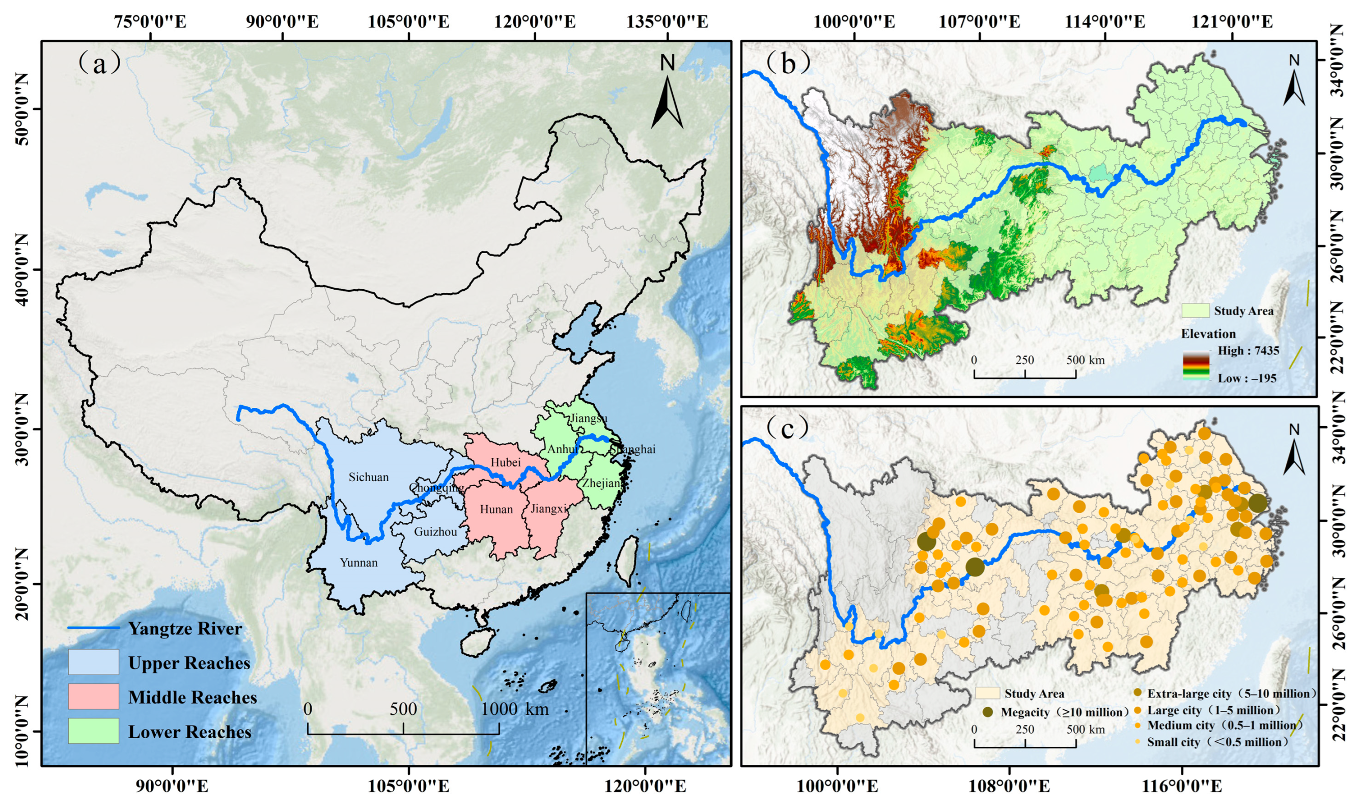
Figure 1. Spatial distribution of 107 sample cities in the YREB: (a) YREB location in China; (b) spatial extent of selected cities; (c) categorized city distribution.
Applsci 15 11175 g001
Figure 2. RSG-Net architecture flow chart.
Applsci 15 11175 g002
Figure 3. RSG-Net model design flow chart.
Applsci 15 11175 g003
Figure 4. Spatiotemporal distribution of total carbon emissions (TCE) across 107 cities in the YREB (2002–2022): (a) 2002; (b) 2007; (c) 2012; (d) 2017; (e) 2022.
Applsci 15 11175 g004
Figure 5. Spatial changes in the urban built-up areas of YREB cities from 2002 to 2022.
Applsci 15 11175 g005
Figure 6. Box plot of urban form landscape pattern index (excluding CA).
Applsci 15 11175 g006aApplsci 15 11175 g006b
Figure 7. Spatial distribution map of indicators of YREB morphological characteristic elements in 2002 and 2022: (a,b) PopDen; (c,d) NDVI; (e,f) RD; (g,h) WAR; (i,j) SI; (k,l) DI; (m,n) TI; (o,p) BLR; (q,r) GDP; (s,t) CLC.
Applsci 15 11175 g007
Figure 8. Heat map showing the correlation between TCE and 14 highly correlated UF indicators.
Applsci 15 11175 g008
Figure 9. Scatter plots illustrating predictions of four distinct models are presented as follows: (a) GBDT, (b) RF, (c) SVR, and (d) RSG-Net. Actual values correspond to CO2 emissions, while predicted values refer to those generated by each model. The dotted line denotes a 1:1 relationship, and the red line represents the trend of each model.
Applsci 15 11175 g009
Figure 10. SHAP plot of four feature importance: (a) overall feature importance, (b) top 15 feature importance, (c) sliding window features importance, and (d) importance of comprehensive static mean features.
Applsci 15 11175 g010
Table 1. Description and sources of data.
Data NamePeriodData DescriptionData SourceFormat
NPP-VIIRS-like nightlight data2002–2022Based on DMSP-OLS and NPP-VIIRS data, with a resolution of 500 m.Harvard DataverseGeoTIFF
ODIAC Fossil Fuel Emission DataIntegrating multi-source data with a resolution of 1 × 1 km.NIES
China 30-m Annual Land Cover DatasetChina’s annual land cover product (CLCD) from 1985 to 2022, with a spatial resolution of 30 m.NCDDC
(https://zenodo.org/records/8176941, accessed on 16 September 2025)
NDVI DatasetCombine these monthly data to generate annual data with a spatial resolution of 1 km.Global Resources Data Cloud(http://www.gis5g.com, accessed on 16 September 2025)
Socioeconomic statistics dataInvolving population, transportation, land, economy, and other aspects.China Urban Statistical YearbookMicrosoft Excel
Administrative
boundaries
2022The provincial and municipal boundaries were derived from the 2022 national boundary dataset.National Basic Geographic
Information Centre (http://www.ngcc.cn, accessed on 16 September 2025)
ESRI Shapefile
Table 2. Description of urban form indicators.
DimensionsIndicatorEquationDescription
LSPISprawlClass areas ( C A ) C A = i = 1 n a i 1 / 1000 a i is area (km2) of urban patch i .
Number of Patches ( N P ) N P = n n is the number of urban patches.
Edge density ( E D ) E D = 10,000 i = 1 n e i / A e i is total edge length (km) of urban patch i .
Extended Nearest Neighbor with Mutual Neighborhood ( E N N _ M N ) E N N _ M N = j = 1 n h i j n i h i j is the Euclidean nearest-neighbor distance of patch i to its closest patch of the same type.
n i is count of patches possessing valid nearest-neighbor relationships.
ComplexityPatch density ( P D ) P D = n / A n is the number of urban patches.
A is total landscape area (km2).
Landscape shape index ( L S I ) L S I = 0.25 j = 1 m k = 1 m e j k * A e j k * is total edge length (km) between patch types j and k .
Mean perimeter-area ratio
( P A R A _ M N )
P A R A _ M N = i = 1 n p i a i A p i is perimeter (m) of urban patch k
a i is area (km2) of urban patch a i .
AggregationLargest patch index ( L P I ) L P I = max i = 1 . . . n a i A A is total landscape area (km2).
Proportion of like adjacencies ( P L A D J ) P L A D J = j = 1 m g j j j = 1 m k = 1 m g j k 100 g j k is number of like adjacencies (joins) between pixels of patch types j and k based on the double-count method.
Patch cohesion index
( C O H E S I O N )
C O H E S I O N =
1 i = 1 n p i * i = 1 n p i * a i * 1 1 Z 1 100
p i * is perimeter of urban patch i in terms of number of cells.
a i * is the area of urban patch i in terms of number of cells.
Z is the total number of cells in the landscape.
UMCPopulationPopulation Density (PopDen) P o p D e n = T o t a l   p o p u l a t i o n / a r e a All indicators of characteristic elements are quantified based on socioeconomic statistical data.
RoadRoad Density (RD) R D = T o t a l   r o a d   l e n g t h / a r e a
LandConstruction Land Concentration (CLC) C L C = L a n d   a r e a   f o r   c o n s t r u c t i o n
/ U r b a n a r e a
Development Intensity (DI) D I = L a n d   a r e a   f o r   c o n s t r u c t i o
/ A d m i n i s t r a t i v e   a r e a
Built-up Land Ratio (BLR) B L R = L a n d   a r e a   f o r   c o n s t r u c t i o n
/ B u i l t u p   a r e a
UMCEconomyGross Domestic Product (GDP) G D P = Added value of primary industry
+ A d d e d   v a l u e   o f   s e c o n d a r y   i n d u s t r y
+ A d d e d   v a l u e   o f   t e r t i a r y   i n d u s t r y
All indicators of characteristic elements are quantified based on socioeconomic statistical data.
Share of Secondary Industry (SI%) S I % = S e c o n d a r y   i n d u s t r y   a d d e d
/ G D P × 100 %
Share of Tertiary Industry (TI%) T I % = T e r t i a r y   i n d u s t r y   a d d e d
/ G D P × 100 %
NaturaWater Area Ratio (WAR) W A R = W a t e r   a r e a
/ t o t a l   a r e a   o f   a l l   l a n d   t y p e s
w i t h i n   t h e   r e g i o n × 100 %
The areas of each land cover category are extracted from the CLCD dataset.
NDVI-Based on monthly data, the average fusion generates annual synthetic data.
Table 3. Model data partition.
Sample SetNumberMin (106 t)Max (106 t)Standard Deviation (106 t)
Training Set1490.5787.3512.70
Test Set650.6531.227.24
Table 4. ACE prediction model for nine provinces and two cities in YREB from 2002 to 2022.
StateRegression Results
Regression EquationR2F Valuep Value
Anhuiy = 88.977x + 46360.918133.9460.00
Guizhouy = 89.173x + 2116.70.917120.9140.00
Hubeiy = 74.804x + 2875.60.87979.6140.00
Hunany = 85.948x + 2604.60.911133.3270.00
Jiangsuy = 105.64x + 8760.80.894134.8330.00
Jiangxiy = 73.209x + 1848.70.90677.2380.00
Shanghaiy = 162.96x + 396.140.942225.6080.00
Sichuany = 55.685x + 2727.70.910121.3930.00
Yunnany = 99.487x + 2654.90.888119.3470.00
Zhejiangy = 77.01x + 58370.87194.3680.00
Chongqingy = 77.01x + 58370.890105.6240.00
Note: x represents the total of the regional night-time light values, and y denotes the total anthropogenic carbon emissions.
Table 5. Total ACE in the YREB and river basin (unit: Mt).
TypeAnnual Total
20022007201220172022
URE60.88104.56146.59149.80171.88
MRE61.19100.91140.17143.25164.38
LRE201.57357.56529.93541.37621.16
TCE323.64563.03816.69834.41957.42
Table 6. Correlation coefficients between TCE and various UF indicators.
TypeIndicators
LSPICANPPDLPIED
0.7400.697−0.244−0.133−0.389
LSIPARA_MNENN_MNPLADJCOHESION
0.6620.089−0.2800.3750.130
UMCPopDenCLCDIBLRRD
0.7930.5120.7060.3190.320
NDVIWARSITIGDP
−0.6090.396−0.0110.4500.855
Disclaimer/Publisher’s Note: The statements, opinions and data contained in all publications are solely those of the individual author(s) and contributor(s) and not of MDPI and/or the editor(s). MDPI and/or the editor(s) disclaim responsibility for any injury to people or property resulting from any ideas, methods, instructions or products referred to in the content.