Deterministic Parameter Control Methods for Genetic Algorithms: Benchmarking on Test Functions and Boost Converter Design Optimisation

Abstract

Genetic Algorithms (GAs) are pillars of evolutionary computing and one of the most well-known population-based metaheuristic optimisation techniques. They are widely used in engineering and applied optimisation problems for their capabilities in finding global solutions. Standard GAs (SGAs) determine probabilities of crossover and mutation by computationally expensive trials. Adaptive Genetic Algorithms (AGAs), on the other hand, improve this process by adjusting the parameters throughout generations. This study proposes three deterministic parameter control functions, ACM1, ACM2 and ACM3, for the regulation of crossover and mutation probabilities. Using advanced test functions, comparisons between four deterministic GAs, an SGA, two fixed-parameter GAs, and an AGA have been made. The fixed-parameter configurations are called FCM1 and FCM2. The AGA is called LTA, and four deterministic methods are called HAM and ACM1–3. Results show that the SGA is mostly inadequate for complex optimisation problems. The LTA performs inconsistently by failing on some functions and succeeding on others. The methods, ACM2, HAM, and FCM2, are highly robust and effective. Unexpectedly, the FCM2 performs the best for smaller population sizes. However, in higher-dimensional problems, the proposed method, ACM2, is superior and shows less variability in finding optimal solutions. The methods are also evaluated using a boost converter implementation.

1. Introduction

The Genetic Algorithm (GA), originally proposed by [1], is a broad term today defining the main class of Evolutionary Computing [2]. GAs are the metaheuristic population-based search algorithms that mimic the process of evolution as a result of Darwin’s principle of natural selection theory in genetics. GAs are easy to apply and offer the advantages of being used for all kinds of variables and objective functions, including discrete optimisation problems, and differ from traditional optimisation methods in many aspects [3,4,5,6,7]. GAs are used for minimising costs and maximising incomes in manufacturing, deciding to design procedures of mechanical components in engineering, prediction of proteins and other molecular structures in biochemistry and medicine, finding optimal routes of vehicles in transportation and distribution networks, resource utilisation and planning in economics, task scheduling in business, determining optimal combination of various variables in finance, optimising operational stages of wireless sensor networks in communication, in addition to many other real-word applications.

The basic idea behind GAs is to create a random set of possible solutions (population) representing different decision variables and then search the global optimum using an iterative process. A GA optimisation starts with a sufficiently large set of candidate solutions, which is composed of the individuals representing possible solutions to the problem in question. Therefore, GAs are started with an initial population of $\mathrm{n}$ randomly selected individuals. After the initial population is created, there is an iterative process that comprises evaluation, selection, crossover, and mutation [8,9].

In the first step of each iteration, called evaluation, the fitness values of individuals are calculated by using a certain fitness function. In the selection step that follows the evaluation process, the parents to be included in the mating pool are selected using a certain selection operator. In the selection, an appropriate fitness-proportionate selection method or a tournament selection method is used. The number of individuals is kept fixed during all the generations of GA, but the individuals with higher fitness values can be selected for one or more times into the mating pool. After the selection step, the parents in the mating pool are randomly selected as pairs and mated using a crossover operator to produce the offspring. The size of the mating pool is determined according to the probability of crossover ($pc$) assigned as a ratio between 0 and 1. Following the crossover of the parents, a certain percentage of offspring are mutated using a probability of mutation ($pm$) varying between 0 and 1. A mutation operator is an essential exploitation tool in GAs because it changes the alleles of some genes of the offspring chromosomes to increase the genetic diversity in the population. In conventional applications of GAs, the pm is a constant in all of the iterations. Consequentially, the same number of offspring are mutated, and the diversity change is not taken into account. The final step in each iteration is creating the population for the next generation using some replacement strategies. The most common replacement strategy is generational replacement, so-called Generational GA (GGA). In the GGA strategy, the new generation is formed after all offspring are obtained. Alternatively, in the Steady-State Generational (SSGA) replacement strategy, a new generation is created as soon as a new offspring is obtained. After the replacement step, the number of generations is incremented by 1, and the user-defined termination condition controls whether to continue or not to the next iteration. Usually, when a user-defined number, called the maximum number of iterations, has been reached, the evolutionary process is terminated, and the fittest solution is returned as the best optimal solution from GA.

In each GA iteration, the average fitness of a population is optimised by crossing individuals with higher fitness values, and by mutating some offspring to generate the genetic diversity along the generations. The gradual improvement for the optimal solution continues until a pre-defined termination condition is satisfied. The fitness values obtained in each generation are compared with the previous best solution to find the optimal solution. As the generations evolve, the number of individuals with higher fitness increases while the individuals with lower fitness are excluded from the population. The research on GAs has shown that crossover is more important in the early stages of a GA run because the search space is wide enough to find an optimal solution. However, as the GA progresses, the search space narrows, and the solutions become similar in subsequent generations of GAs. This may lead to a tendency to get stuck at a local optimum. This is an important problem, called premature convergence in the GAs. The insufficient population size, the increase in similar individuals due to selection, the loss of some good alleles due to crossover, and parameter settings with improper mutation and crossover rates are possible causes of premature convergence. All these factors lead to a decrease in genetic diversity and a disproportionate exploitation or exploration balance [10]. When premature convergence occurs, the search process cannot escape from a local optimum, and the global optimum will not be reached. There are ways to overcome this problem by increasing the diversity or expanding the search space. It can be useful to dynamically set or control the exploitation and exploration levels for a GA [2]. For this, an appropriate setting should be established between a broad search and a fast improvement.

To tune crossover or mutation rates in Genetic Algorithms, several methods and techniques have been developed [11]. According to Eiben et al. [12], the methods for parameter setting are classified into three groups: (I) deterministic methods, (II) adaptive methods, and (III) self-adaptive methods. A Genetic Algorithm that controls and adapts $pc$ and $pm$ in each generation is called the Adaptive Genetic Algorithm (AGA). Instead of using fixed values for $pc$ and $pm$, an AGA utilises the population information in each generation and adaptively regulates the $pc$ and $pm$ to maintain the population diversity in addition to the convergence capacity. The deterministic methods follow pre-defined rules or mathematical functions to change parameters over generations without receiving feedback from the search process. Adaptive methods utilise feedback for parameter regulation, using information on the minimum, maximum, and average fitness of the population. When it comes to self-adaptive methods, the control parameters are encoded within the chromosome and evolve with the solution variables. As each individual carries its own crossover and mutation values, updated through genetic operations, the algorithm can autonomously find the optimal settings.

On the feedback concept in Evolutionary Algorithms, researchers have come up with smarter ways that go beyond just minimum, maximum, and average fitness of the population. Such methods utilise additional feedback mechanisms such as diversity, information entropy, and fitness differences, among others. For example, in [13], the population diversity is used as feedback for regulating parameters like crossover, mutation rate, or tournament size. In [14], a rank-based feedback approach is taken based on the fitness values of individuals. Norat et al. employ self-adaptive feedback [15] using fitness differences between parent and offspring, as well as the search states to adjust crossover and mutation parameters. Another feedback mechanism that attracts researchers’ attention is information entropy, which measures the variability or uncertainty within the population or at specific genetic loci [16,17,18,19]. In other words, entropy-based adaptive parameter control evaluates both the trends within the population and the state of individual genes. As a result, the possibility of premature convergence is greatly reduced while diversity is maintained.

Many researchers have also addressed the problem of parameter tuning over the years. For example, the Controlled Random Search (CRS) algorithm [20] employs a stochastic, sampling-based approach that can be utilised for parameter configurations. The F-Race method [21] takes a statistical racing approach, using non-parametric statistical tests to compare parameter configurations and eliminate the ones that perform worse. The Relevance Estimation and Value Calibration (REVAC) method [22] offers an alternative to the statistical approaches by taking an entropy-based approach to estimate the distribution of promising parameter configurations. The method ParamILS (Parameter Iterated Local Search) [23] introduces a stochastic, iterated local search-based approach for parameter tuning and can be particularly advantageous for discrete and categorical parameters.

One of the objectives of this study is to address the premature convergence problem in GAs. For this, deterministic parameter control methods that adjust the crossover and mutation probabilities are proposed and compared to the SGA, two fixed-parameter GAs, and an AGA. The fixed-parameter GAs are called Fixed Crossover and Mutation setting 1 (FCM1) and Fixed Crossover and Mutation setting 2 (FCM2). The FCM1 and FCM2 consider two configurations: $pc=0.5, pm=0.5,$ and $pc=0.8, pm=0.2$, respectively. With the FCM2 configuration, we aimed to create a balanced exploration–exploitation trade-off, particularly for scenarios with small population sizes, where neither operator should dominate the search process. The rest of the methods involve both adaptive and deterministic approaches. The adaptive approach is from [24], referenced as LTA: Lei and Tingzhi’s Adaptive Method, in this study. The deterministic approach is a dual method—Decreasing High Crossover and Increasing Low Mutation (DHC/ILM) rate and Increasing Low Mutation and Decreasing High Crossover (ILM/DHC) by Hassanat et al. [25]—which will be referred to as HAM: Hassanat’s Method throughout the rest of this paper. For the novel methods in this study, we investigated the deterministic methods due to their computational efficiency and straightforward structures for parameter adaptation. They employ pre-defined functions that do not need additional tuning during the search process. Therefore, the deterministic approaches prove to be highly attractive for real-world applications where limitations on computational power are often restrictive. The proposed methods are named as follows: A Crossover and Mutation function 1 (ACM1), A Crossover and Mutation function 2 (ACM2), and A Crossover and Mutation function 3 (ACM3).

The contributions and novelties of this study can be summarised as follows:

▪

This paper proposes three novel deterministic parameter control functions (ACM1, ACM2, ACM3) for regulating crossover and mutation probabilities across generations.

▪

A broad performance comparison study utilising a diverse group of unimodal and multimodal benchmark functions was carried out in three sets of experiments evaluating a standard GA, an adaptive GA, two fixed-parameter GAs, and four deterministic GAs.

▪

The comparisons were verified with statistical tests and Monte Carlo (MC) trials; several cases, such as varying population sizes (20, 50, 100) and problem dimensions, were considered, creating a substantial set of results.

▪

Although the benchmarking functions included some of the most difficult optimisation problems, a simple boost converter implementation was used to evaluate the methods, as well. A unique fitness function has been formulated. This is also the first time the proposed methods have been implemented on an engineering problem.

The remainder of this paper is organised as follows. Section 2 investigates the related works from the literature in detail, discussing some of the shortcomings and potential research gaps. Section 3 introduces the materials and methods, including the computing environment and tools, and test functions used for evaluations. The section continues by explaining the three sets of experiments and ends with the description of the proposed methods. Section 4 presents the results, and Section 5 discusses the implications of the results. Section 6 concludes the paper by summarising key points and discussing future work.

2. Related Works

In GAs, the parameter $pm$ is increased when fitness values tend to converge to a local optimum or is decreased when the search space starts to narrow. The $pc$ is processed in the same way but in the opposite direction. The procedure of setting these parameters is called parameter setting. According to the classification by [12], there are two main types of parameter setting in GAs: (I) parameter tuning; (II) parameter control. The first one depends on running a GA with different levels of $pc$ and $pm$, and then selecting a combination of these parameters to give the best results to initiate the final run of GA. In this approach, a constant value for $pc$ and $pm$ are used during all of the generations. On the other hand, with the parameter control approach, the parameters $pc$ and $pm$ are determined while the GA runs continue evolving.

In SGA, the parameters $pc$ and $pm$ are set to some constant values in the range of $[0,1]$, and remain the same for all generations. When a high $pm$ value is selected, many genes of the offspring will be mutated. In such a case, it may cause a change for the worse in fitness values due to the deterioration caused by high mutation rates in the genes of individuals with better fitness values. However, if the genes of the individuals have become similar to each other, high mutation can also lead to improvement with the formation of genes that create better fitness values. On the other hand, with a low probability of mutation, very few offspring’s genes undergo mutation. In this case, individuals with better fitness are only slightly affected by small random mutations, but it may lead to an improvement in the fitness values of individuals with worse fitness. In both cases, there is no significant increase in the average fitness of the population. A GA designer needs to set an appropriate $pm$ value for the optimisation problem with the SGA. In SGAs, the parameters $pm$ and $pc$ are set as constant in different levels. For example, the parameter setting with a small $pm$ of 0.05 and a high $pc$ of 0.9 may be well-suited for saving the better fitness solutions but not contribute much to the individuals with worse fitness values. In another case, the parameters $pm$ and $pc$ are set to 0.2 and 0.8, respectively, and may give better results for the individuals with worse fitness values. The best parameter values of $pm$ and $pc$ are determined by trial-and-error experiments, or by adopting the parameters reported in similar works. Note that this approach increases computational cost because it requires many experiments for different setting combinations of the parameters $pm$ and $pc$.

As described above, applying the parameters $pm$ and $pc$ at constant rates provides an equal opportunity for the impairment of the better fitness values and for the improvement of the poorer fitness values. To maintain individuals with good fitness, the mutation is required to change the genes of the individuals with poor fitness. As one of the methods based on this idea, Srinivas and Patnaik [26] proposed an algorithm that includes the formulas shown in the equations below:

$${pc}_a=\left\{\begin{array}{c}{pc}_1{\displaystyle \frac{f_{max}-f^{\prime }}{f_{max}-f_{avg}}}, {\mathrm{if} f}^{\prime }\ge f_{avg}\\ \hspace{1em}\hspace{1em}\hspace{1em}\hspace{1em}{pc}_2, \mathrm{otherwise}\end{array}\right.,$$

(1)

$${pm}_a=\left\{\begin{array}{c}{pm}_1{\displaystyle \frac{f_{max}-f}{f_{max}-f_{avg}}}, if f\ge f_{avg}\\ \hspace{1em}\hspace{1em}\hspace{1em}\hspace{1em}{pm}_2, \mathrm{otherwise}\end{array}\right..$$

(2)

The notations belonging to Equations (1) and (2) are listed as follows:

${pc}_a$: Dynamic crossover probability;

${pm}_a$: Dynamic mutation probability;

${pc}_1$: $pc$ for case 1: ($0\le pc1\le 1$; usually set to $0.5$);

${pc}_2$: $pc$ for case 2: ($0\le pc2\le 1$; usually set to $0.9$);

${pm}_1$: $pm$ for case 1: ($0\le pm1\le 1$; usually set to $0.2$);

${pm}_2$: $pm$ for case 2: ($0\le pm2\le 1$; usually set to $0.01$);

$f_{avg}$: Average fitness value;

$f_{min}$: The lowest fitness value;

$f_{max}$: The highest fitness value;

$f^{\prime }$: The fitness value of the crossed individuals with higher fitness;

$f$: The fitness value of the mutated individuals.

According to Equations (1) and (2), if the fitness is greater than or equal to the average fitness then the solution is considered good fitness and a low level of $pm$ is dynamically applied for it. When this method is applied, the individuals with fitness values below the average will have a high level of $pm$ while individuals with fitness above the average threshold will have a low mutation rate.

Based on the results of [26], some researchers proposed improved self-adaptive GAs [27,28,29,30,31]. Among these works, a promising representation of the adaptive crossover and mutation probabilities [31] is shown below:

$${pc}_a=\left\{\begin{array}{c}{pc}_1{\displaystyle \frac{f_{max}-f_{c }}{f_{max}-f_{min}}} ; \mathrm{if} f_{c }\ne f_{max, }{f}_{min}\\ {pc}_2; \mathrm{if} f_{c }=f_{min }\\ {pc}_3; \mathrm{if} f_{c }=f_{max }\end{array}\right.,$$

(3)

$${pm}_a=\left\{\begin{array}{c}{pm}_1{\displaystyle \frac{f_{max}-f_{c }}{f_{max}-f_{min}}} ; \mathrm{if} f_{c }\ne f_{max, }{f}_{min}\\ {pm}_2; \mathrm{if} f_{c }=f_{min }\\ {pm}_3; \mathrm{if} f_{c }=f_{max }\end{array}\right.,$$

(4)

where ${pc}_a$ and ${pm}_a$ are the crossover and mutation probabilities, $f_{c }$ is the one with higher fitness of the first two parents of the crossover operation, and $f_{max}$ and $f_{min}$ are the maximum and minimum fitness in the population, and ${pc}_1$, ${pc}_2$, ${pc}_3$ as well as ${pm}_1$, ${pm}_2$, and ${pm}_3$ are constants between 0 and 1, and ${pc}_2>{pc}_3$ and ${pm}_2>{pm}_3$. Adapting the algorithm for three different fitness levels, such as low, medium, and high, allows for more nuance and potentially leads to converging values in later iterations.

Although [26] and its extended variants adapt the parameters $pm$ and $pc$ according to the fitness of individuals, there is a lack of cooperation with other individuals. As the individuals do not take into account each other, it may be overlooked if some of them are already fitted at a local optimum. Individual fitness values also increase the computational load since the crossovers and mutations require control at each instance. As an alternative solution, Lei and Tingzhi [24] presented an adaptive method (referred to as LTA in this paper) shown in the equations below:

$${pc}_a=\left\{\begin{array}{c}{{pc}_1\left(1-{\displaystyle \frac{f_{min}}{f_{max}}}\right)}^{-1}, {{\mathrm{if} f}_{avg}/f}_{max}>a \mathrm{and} {f_{min}/f}_{max}>b\\ {pc}_2, \mathrm{otherwise}\hspace{1em}\hspace{1em}\hspace{1em} \end{array}\right.,$$

(5)

$${pm}_a=\left\{\begin{array}{c}{{pm}_1\left(1-{\displaystyle \frac{f_{min}}{f_{max}}}\right)}^{-1}, \mathrm{if} {f_{avg}/f}_{max}>a \mathrm{and} {f_{min}/f}_{max}>b\\ {pm}_2, \mathrm{otherwise}\hspace{1em}\hspace{1em}\hspace{1em} \end{array} \right.,$$

(6)

where $a$ is a threshold value between 0 and 1 ($0\le a\le 1$), and the parameter $b$ is a threshold value between 0.5 and 1 ($0.5\le b\le 1$). For clarification, it should be noted that the LTA is a non-deterministic method.

In deterministic GAs, probabilities of crossover and mutation are defined by a deterministic function. Hassanat et al. [25] proposed a dual deterministic approach (referred to as HAM in this paper): Decreasing High Crossover and Increasing Low Mutation (DHC/ILM) rate, and Increasing Low Mutation and Decreasing High Crossover rate (ILM/DHC) rate. Note that the formulas for DHC/ILM and ILM/DHC mirror each other in the opposite direction. The formula of HAM is given below:

$$ilm = L/G,$$

(7)

$$dhc=1-L/G,$$

(8)

where $L$ is the current generation number, $G$ is the number of generations,$ilm$ and $dhc$, are the rates of mutation and crossover in the $L^{th}$ generation of GA, respectively. HAM increases the $\mathrm{i}\mathrm{l}\mathrm{m}$ and decreases the $\mathrm{d}\mathrm{h}\mathrm{c}$ linearly as the generations progress (illustrated later in Section 3). According to Equation (7), if $G$ is 100, the $ilm$ is calculated as 0.01, 0.1, 0.5, 0.75, and 1.0 at the 1st, 10th, 50th, 75th, and 100th generations, respectively. For the same generations, if $G$ is set to 20, the number of offspring to be mutated will be 0, 2, 10, 15, and 20, respectively. This means that the number of individuals to be mutated will be 0 in the earlier generations due to the small value of $G$. As none of the offspring mutates in early generations when $G$ is too small, this is clearly a disadvantage of HAM.

The recent advances in Evolutionary Algorithms (EAs) report that Differential Evolution (DE) methods with adaptive parameter control are leading in performance benchmarking. Among the variations in the DE, Yu et al. [32] introduced Two-Level Parameter Adaptation, F (Factor), and CR (Crossover Probability) to maintain diversity while achieving convergence by also using population distribution to detect exploration–exploitation phases. Wang et al. [33] proposed a Parameter and Strategy Adaptive Differential Evolution (APSDE) algorithm where both mutation strategy and control parameters are optimised adaptively accompanied by a population of suboptimal individuals. According to the authors, accompanying population enhances diversity by reverse individual generation and a radial spatial projection approach for tacking evolutionary direction. APSDE’s competitiveness were validated by the IEEE CEC benchmarking underlining the strengths of the method, which are adaptive mechanism and improved population diversity. As an additional example, Cheng et al. [34] proposed a CR generation method using fitness z-scores where individuals with lower fitness scores were assigned smaller CR values and vice versa. Takahama and Sakai [35] combines two different techniques to improve the JADE (adaptive DE with optional external archive) method: (I) Estimating whether the population is moving or converging; (II) DE parameter control of extreme individuals.

One of the milestones for adaptive DEs is the Success-history-based Parameter Adaptation for Differential Evolution (SHADE) method and its Linear Population Size Reduction (LPSR) extension (LSHADE) developed by Tanabe and Fukunaga in [36] and [37], respectively. LSHADE, also known for its success in IEEE CEC competitions, combines two mechanisms: (I) SHADE, which learns and stores successful F and CR values across generations; (II) LPSR, which progressively decreases the population size during the search to alternate from exploration to exploitation. Owing to its success, several variants of the method came out. For example, LSHADE-SPACMA by Mohamed et al. [38] is a hybrid framework, which combines LSHADE-SPA (LSHADE Semi Parameter Adaptation) and CMA-ES (Covariance Matrix Adaptation Evolution Strategy). More recently, Fu et al. [39] modified the LSHADE-SPACMA with a novel mutation and archive mechanism improving the method’s exploitation capability, convergence speed, and evolutionary direction.

DE-based methods demonstrate the potential of adaptive parameter control for EAs. However, these methods often need population-level metrics and additional algorithmic procedures that are computationally expensive. Meanwhile, the ACM1–3 methods proposed in this study adopt a deterministic parameter control approach under the GA framework offering a simpler but effective alternative, which would be particularly useful for applications where only limited computational resources are available or real-time performance is needed.

3. Experimental Setup and Benchmarking Methodology

3.1. Computing Environment and Tools

In this study, all experiments have been carried out using R version 4.5.0 [40] and the functions implemented in the R package ‘adana’ version 1.1.0 [41]. The codes of the test functions in

Table 1. Test functions.

FN#	Test Function	Formula
FN1	Aluffi-Pentini	$f\left(x\right)={0.25x}_1^4-{0.5x}_1^2+0.1x_1+0.5x_2^2$
FN2	Dixon-Price	$f\left(x\right)={\left(x_1-1\right)}^2+\sum _{i=2}^{d}i {({2x}_i^2-x_{i-1})}^2$
FN3	Drop-Wave	$f\left(x\right)=-\left(1+\mathit{cos}\left(12{(x_1^2+x_2^2)}^{0.5}\right)/\left(0.5\left(x_1^2+x_2^2\right)+2\right)\right)$
FN4	Himmelblau	$f\left(x\right)={\left(x_1^2+x_2-11\right)}^2+{\left(x_1+x_2^2-7\right)}^2$
FN5	Matyas	$f\left(x\right)=0.26\left(x_1^2+x_2^2\right)-0.48x_1{x}_2$
FN6	Michalewicz	$f\left(x\right)=-\sum _{i=1}^d\mathit{sin}\left(x_i\right){sin}^{2m}(i{x}_i^2/\pi )$
FN7	Rastrigin	$f\left(x\right)=10d+\sum _{i=1}^d(x_i^2-10cos(2\pi x_i\left)\right)$
FN8	Rosenbrock	$f\left(x\right)=\sum _{i=1}^{d-1}{100\left(x_{i+1}-x_i^2\right)}^2+{\left(x_i-1\right)}^2$
FN9	Styblinski-Tang	$f\left(x\right)=1/2\sum _{i=1}^d\left(x_i^4-16x_i^2+5x_i\right)$
FN10	Zettl	$f\left(x\right)={\left(x_1^2+x_2^2-2x_1\right)}^2+0.25x_1$

have been retrieved from the Virtual Library of Simulation Experiments [42] and the R package ‘smoof’ [43], and they are used as the fitness functions in the experiments 1 and 2. A custom R script has also been written in order to apply the Monte Carlo (MC) experiments for performance comparison of the methods.

3.2. Test Functions

In optimisation research, it is customary to make a performance comparison of a proposed algorithm with related or well-established algorithms. In such comparative studies, researchers often use various test functions (or benchmarking functions) whose properties, such as boundaries, local optima, and global optimum, are already known. The test functions belong to different classes of modality, separability, and scalability; therefore, they present different difficulties for continuous optimisation problems [43]. For instance, the multimodal test functions having multiple local optima are useful to test the performance of an algorithm to find the global optimum. On the other hand, the scalable test functions help evaluate the success of an algorithm in the case of an increasing number of decision variables.

In this study, the performances of the compared algorithms are revealed via the simulations with ten test functions. The functions are adopted from a comprehensive survey by [44]. Their formulas are given in Table 1, and their properties are listed in

Table 2. Properties of the test functions.

FN#	Class *	Boundaries	Global Minimum
FN1	UM, S	$[-10,10]$	$f(-1.0465, 0)\approx -0.3524$
FN2	UM, NS	$[-10,10]$	$f\left(2\right((2i-2)/2i)=0$
FN3	UM, NS	$[-5.12,5.12]$	$f\left(\mathrm{0,0}\right)=-1$
FN4	MM, NS	$[-5,5]$	$f\left(\mathrm{3,2}\right)=0$
FN5	UM, NS	$[-10,10]$	$f\left(\mathrm{0,0}\right)=0$
FN6	UM, NS	$[0,\pi ]$	$f\left(2.202906, 1.570796\right)\approx -1.8013$
FN7	MM, S	$[-5.12,5.12]$	$f\left(\mathrm{0,0}\right)=0$
FN8	UM, NS	$[-30,30]$	$f(1,\dots ,1)=0$
FN9	MM, NS	$[-5,5]$	$f(-2.903534,-2.903534)=-78.332$
FN10	UM, NS	$[-5,10]$	$f(-0.0299, 0)=-0.003791$

* S: Separable, NS: Non-separable, UM: Unimodal, MM: Multimodal.

. Although the test functions are selected to represent each modality class in harmony, they create a rigid testing ground because the majority of them are non-separable, as shown in Table 2.

The first function on the list, Aluffi-Pentini, is a unimodal and separable function presenting a relatively basic optimisation task. The second function, Dixon-Price, is also unimodal but non-separable; therefore, due to interactions between variables, it presents moderate difficulty. The Drop-Wave function, despite being unimodal, has a steep and oscillatory surface which may mislead the search of optimisation algorithms. As a multimodal, non-separable function, the Himmelblau contains multiple local minima, making global convergence challenging. The Matyas function is unimodal and non-separable, with a smooth, symmetric surface. The Michalewicz’s function is unimodal and non-separable but is characterised by narrow valleys and steep ridges, making it one of the more difficult benchmarks. The Rastrigin function is multimodal and separable, with a large number of regularly distributed local minima. Also known as the narrow valley problem, the Rosenbrock function is unimodal, non-separable, and is particularly sensitive to algorithm stability. Styblinski-Tang features deep valleys and multiple local minima and is a multimodal and non-separable function. The Zettl function is unimodal and non-separable, with a relatively simple structure.

3.3. Experiments with Test Functions

3.3.1. Experiment 1

In the first experiment, the $pc$ and $pm$ for SGA are set to the typically applied rates of 0.95 and 0.05, respectively. We also test two different configurations to examine the impact of using $pc$ and $pm$ values outside their typical ranges.

For the first fixed-parameter configuration, FCM1, $pc$ is set to 0.8 and $pm$ to 0.2. In the second fixed-parameter configuration, FCM2, both $pc$ and $pm$ are set equally to 0.5 to maintain a balanced level of diversity in the population’s average fitness. This setting was assumed to improve the fitness of individuals with poorer fitness values.

The adaptive method, LTA, and four deterministic methods (HAM, ACM1, ACM2, and ACM3) have also been used for performance comparison.

When optimal solutions of a GA already exist within the initial population, the algorithm may converge faster with larger populations. Despite this advantage, working with large populations increases computational cost and execution time. Therefore, an algorithm can be considered to be more effective if it achieves faster solutions in smaller populations for the same problem. For this reason, this study also aims to evaluate the compared methods under different population sizes to determine the impact of smaller population sizes. The experiments are conducted on test functions with two dimensions (decision variables) using population sizes of 20, 50, and 100. For generating the initial populations, the lower and upper bounds of each decision variable are set to the default values of the test functions listed in Table 2.

The tournament selection with a tournament size of 2 was selected for the competing individuals from the parent population to build the mating pool. Two random parents from the mating pool are then selected to generate the offspring, using the Whole Arithmetic Crossover (WAX) operator [45]. The selection is repeated until the number of offspring reaches the current population size $n$. After the crossover, the Non-Uniform Mutation (NUNIMUT) operator [46] is used to mutate some random offspring.

To replace the current generation, the generational GA with the elitist strategy is preferred as the GA replacement method. In the replacements, the best five parent individuals are retained in the population for the next generation for accelerated improvement of the average fitness of the population. The maximum number of generations is set to 50 and also used as the termination criterion for all GA runs. According to the Central Limit Theorem in statistics, the distribution of sample means attains a normal distribution ignoring the distribution of the original population from which the samples are drawn. Although the higher sample sizes will be more likely representative of the population [47,48], the sampling size of 30 is typically considered a threshold for deciding an appropriate statistical test type, such as the Z-test or t-test [49]. In this study, we adopt this minimum threshold level in order to work with a sufficient sample size on the one hand, and, to avoid long execution times on the other. For this reason, all experiments use Monte Carlo with 30 trials for comparing the significant differences between the average of best solutions of examined methods.

To make sure the comparisons are fair, the same initial population was used for all methods in each run of the MC simulations. The mean, median, best, worst, and the standard deviation of the best solutions for each algorithm are calculated based on the results of MC simulations. In addition to the descriptive statistics, the Number of Convergence to Global Optimum (NCGO) is counted during MC simulations to evaluate the overall performance of each compared method. A summary of parameter settings for Experiment 1 and Experiment 2 is provided in

Table 3. Parameter settings used in Experiment 1 and Experiment 2.

Parameter	Experiment 1	Experiment 2
Population size (n)	20, 50, 100	25 × d (d = 5, 10, 15)
Dimension (d)	2	5, 10, 15
Max generations	50	5 × n
Crossover rate (pc)	Determined with the algorithms	Determined with the algorithms
Mutation rate (pm)	Determined with the algorithms	Determined with the algorithms
Runs (MC trials)	30	30
Selection method	Tournament selection (size = 2)	Same as Experiment 1
Crossover operator	Whole Arithmetic Crossover	Same as Experiment 1
Mutation operator	Non-Uniform Mutation	Same as Experiment 1
Elitism	Best 5 parents retained each generation	Same as Experiment 1
Termination criteria	Max generation = 50	Max generation = 5 × n
Initialisation	Random within function bounds	Random within function bounds

.

3.3.2. Experiment 2

Experiment 2 aims to compare the performances of the methods on the Dixon-Price, Rastrigin, and Rosenbrock test functions (FN4, FN7, and FN8 in Table 1, respectively) for different dimensions of data. These functions are widely used for assessing parameter control due to their varying landscape characteristics and scalability. Using these representative functions allows us to analyse the impact of dimensionality ($d=5$, $d=10$, $d=15$) on the methods while keeping the computational cost manageable.

As in the Experiment 1, the statistics from the test function evaluations are calculated after 30 repeated runs of GA for each method. For each dimension, the initial population sizes (n) are determined using the formula $n=25d$ and the maximum number of iterations is chosen as $5n$. The remainder of the parameter settings are consistent with Experiment 1 (see Table 3).

3.3.3. Experiment 3

In order to compare the performances of the examined Genetic Algorithm methods on a real-world engineering problem, a fitness function was developed for the optimisation of a boost converter. A boost converter is a device that transforms a lower voltage input from a Direct Current (DC) power source (e.g., a Li-ion battery or solar cell), to a higher DC output voltage. For this reason, they are also known as step-up converters.

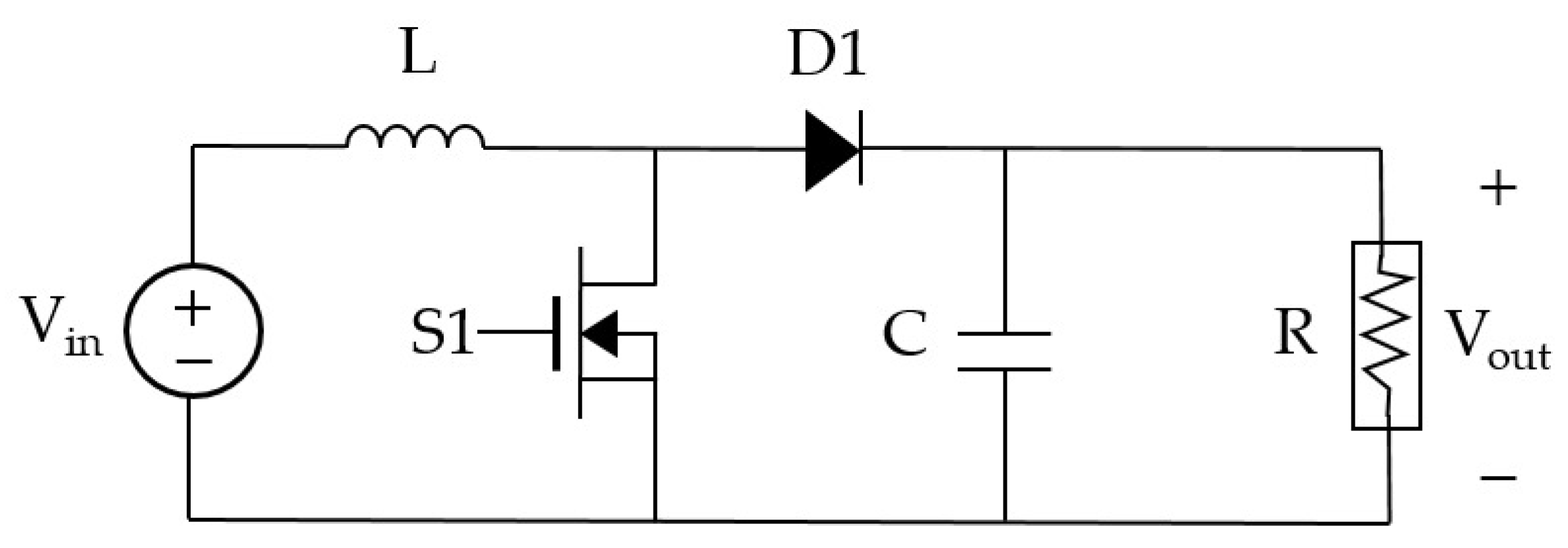
In this experiment, the boost converter is adapted from the example in Chapters 2 and 3 of [50]. The converter circuit diagram, which uses a Metal–Oxide–Semiconductor Field-Effect Transistor (MOSFET) as its switching device ($\mathrm{S}1$), is illustrated in Figure 1.

$\mathrm{S}1$ works as a switch, allowing the energy storage or flow within the circuit. The remaining circuit elements comprise the inductor ($L$), diode ($D1$), capacitor ($C$), and the load resistance $\left(R\right)$, where the input voltage and the output voltage are $V_{in}$ and $V_{out}$, respectively. The inductor and the capacitor enable the storage and release of the electric current, and the diode ensures of its direction.

The converter model is further described with the following equations. The output voltage is calculated by the boost converter voltage conversion ratio as in Equation (9),

$$V_{out}={\displaystyle \frac{V_{in}}{1-D}},$$

(9)

where $D$ is the duty cycle, the fraction of on-time vs. off-time of the transistor. The output current is given by

$$I_{out}={\displaystyle \frac{V_{out}}{R}}.$$

(10)

The inductor current ripple is computed using Equation (11),

$$I_r={\displaystyle \frac{V_{in}D}{f_{sw}L}},$$

(11)

where and $f_{sw}$ is the switching frequency. The parameter $f_{sw}$ determines how fast the switching takes place. The capacitor voltage ripple is formulated as in Equation (12):

$$V_r={\displaystyle \frac{I_r}{8f_{sw}C}}.$$

(12)

The converter’s efficiency ($\eta$) is modelled by including conduction losses ($P_{cond})$ and switching losses $P_{sw}$:

$$\eta =\left\{\begin{array}{c}\hspace{1em}\hspace{1em}\hspace{1em}\hspace{1em}\hspace{1em} 0,\hspace{1em} \mathrm{if} P_{out}\le 0\\ {\displaystyle \frac{P_{out}}{P_{out}+P_{cond}+P_{sw}}}. \mathrm{otherwise}\end{array}\right.$$

(13)

The parameter $P_{out}$ stands for the output voltage:

$$P_{out}=I_{out}{V}_{out}.$$

(14)

The conduction losses are calculated as

$$P_{cond}={I_{rms}}^2{R}_{eq},$$

(15)

where $I_{rms}$ is the rippled induced RMS current estimate,

$$I_{rms}=\sqrt{{I_{out}}^2+{\displaystyle \frac{{I_r}^2}{12}}},$$

(16)

and $R_{eq}$ is the equivalent series resistance which will be assumed $0.05\Omega$ in this study. The switching losses are formulated in

$$P_{sw}=k_{sw}{f}_{sw}{I}_{out}{V}_{out},$$

(17)

where it is assumed that the value of $k_{sw}=5\times {10}^{-8}$.

The design parameters of the example are defined in

Table 4. Converter design parameters and limits.

Notation	Parameter	Symbol	Constraints
$R$	Resistance	$\Omega$	$\left[1,100\right]$
$L$	Inductance	$\mathrm{H}$	$\left[1\times {10}^{-6},1\times {10}^{-3}\right]$
$C$	Capacitance	$\mathrm{F}$	$\left[1\times {10}^{-6},1\times {10}^{-3}\right]$
$V_{in}$	Input Voltage	$\mathrm{V}$	$\left[5,20\right]$
$D$	Duty Cycle	$\mathrm{D}$	$\left[0.1,0.9\right]$
$f_{sw}$	Switching Frequency	$\mathrm{H}$z	$\left[2\times {10}^4,1\times {10}^6\right]$

where the lower and upper bounds of the parameters are defined as constraints.

The working principles of a boost converter are relatively straightforward. However, it is a highly non-linear model with lots of interactions between the parameters, and therefore, it can be challenging to design. The specific purpose of the experiment is to let the examined GAs find the optimal design parameters to achieve the desired $V_{out}$, minimise Voltage Ripple ($V_r$), and maximise the efficiency of conversion $\left(\eta \right)$ under the limitations of the circuit components. By adjusting the parameters in Table 4, the GA optimisers search the design space to minimise deviations from the reference values. For this purpose, we have formulated the GA fitness function as in

$$F\left(x\right)=w_v{\displaystyle \frac{\left|V_{out}\left(x\right)-V_{ref}\right|}{V_{ref}}}+w_r{\displaystyle \frac{\left|V_r\left(x\right)-V_{ref,r}\right|}{V_{ref,r}}}+w_{\eta }{\displaystyle \frac{\left|\eta \left(x\right)-{\eta }_{ref}\right|}{{\eta }_{ref}}}+\theta \left(x\right)$$

(18)

where $w_v$, $w_r$, and $w_{\eta }$ denote the weighting coefficients for voltage, ripple, and efficiency set-point (reference) errors, respectively. The references values for the same order are defined as $V_{ref}$, $V_{ref,r}$, and ${\eta }_{ref}$. The weighting coefficients are set to $w_v=1$, $w_r=5$, and $w_{\eta }=3$, reflecting common converter design practices, where ripple suppression is typically emphasised since the ripple is determined by intrinsic design choices that cannot be altered after the converter has been built. Unlike the ripple, the output voltage can be further corrected for absolute regulation using feedback control mechanisms. The ripple also affects the efficiency, hence justifying the choice of weighting coefficients. Each tracking error was normalised with respect to its reference value for balanced solutions. The reference values are selected as $V_{ref}=12\mathrm{V}$, $V_{ref,r}=0.1\mathrm{V}$, and ${\eta }_{ref}=0.90$. The term $x=[R, L, C, V_{in}, D, f_{sw}]$ represents the converter design parameter vector. Lastly, $\theta \left(x\right)=\sum _i^m{\varphi }_i\left(x_i\right)$ is the overall penalty term obtained by the sum of $m$ individual penalties. The penalty corresponding to the $i$-th design parameter $x_i$ is defined by

$${\varphi }_i\left(x_i\right)=\left\{\begin{array}{c}0, \mathrm{if} x_i\in \left[x_{i,min},x_{i,max}\right]\\ \lambda , \mathrm{otherwise}\hfill \end{array}\right.,$$

(19)

where the constant $\lambda$ is set to 1000, a significantly large value, to make sure that any violation of the constraints affects the fitness score dramatically.

Using the fitness function $F\left(x\right)$ in Equation (18), GAs in comparison will be run for a population size of $n=50$ over 200 generations, as well as 30 independent MC simulations. During the MC simulations, the same initial population was used for each GA method to ensure a fair comparison takes place. Finally, the mean, median, best, worst, and standard deviations of the results from each algorithm will be computed. In this experiment, all individuals are represented using real-valued vectors for all design parameters seen in Table 4.

3.4. Statistical Tests and Performance Ranking

During the comparisons, GAs are run 30 times with different initial populations. The statistics of mean, median, standard deviation, best, and worst fitness values of each GA run are saved for use in the statistical tests. Preliminary tests showed that some MC trials were not normally distributed; thus, the parametric test assumptions could not be met. Therefore, in this study, the medians of solutions are used instead of arithmetic means to compare the performance of methods. In order to test the statistical significance of the differences between the median of solutions, the non-parametric one-way Kruskal–Wallis Test (KWT) has been applied on each test function after the GA runs [51]. As the post hoc test, the pairwise Wilcoxon Signed Rank Sum Test (PWRST) with Family-Wise Error Rate (FWER) adjustment method can be applied after KWT. In this paper, the PWSRTs are performed with False Discovery Rate (FDR) adjustment under a two-sided null hypothesis with type I error of 0.05.

In addition to the pairwise comparison tests, the NCGOs are also calculated for the ranks of compared methods. To calculate the NCGOs of the compared methods, the minimum difference of $1\times {10}^{-3}$, has been taken as the convergence value for each test function. If the difference between the global optimum of the examined test function and the best solution found with a GA run is less than or equal to this minimum difference, it is assumed that the algorithm has found the global optimum of the test function. To evaluate the performance of the algorithms, the NCGOs are ranked for each test function using the average ties method for the same NCGO. The overall sum of the ranks is computed for each algorithm, and the algorithms with a smaller overall rank sum are considered more successful when compared to those with a higher rank sum.

3.5. Proposed Methods

Three novel deterministic methods are proposed for adjusting mutation and crossover rates in this study. The first one of these methods, called A Crossover and Mutation function 1 (ACM1), sets the parameter $pm$ using a fraction of a sinusoidal wave function in the range of [0, 1] as shown in Figure 2b.

The crossover and mutation rates for the $g^{th}$ generation in ACM1 are calculated by

$${pm}_g=\mathit{sin}\left({\displaystyle \frac{g}{g_{max}}}\right)+0.15,$$

(20)

$${pc}_g=1-{pm}_g.$$

(21)

where $g_{max}$ is the number of generations. The term ${g/g}_{max}$, is a ratio between 0 and 1. Equation (20) is designed to ensure that the minimum value of ${pm}_g$ is 0.15, so that a decent rate of mutation is guaranteed in the case of a relatively large $g_{max}$. As a result, the ACM1 can tackle the zero-mutation handicap of method HAM, against a large number of generations (recall Section 2). Equation (21) shows the relationship between the crossover rate, ${pc}_g$, and the mutation rate, ${pm}_g.$

The second proposed method, called A Crossover and Mutation function 2 (ACM2), applies a non-linear increase for $pm$ as seen in Figure 2c, as an alternative mathematical approach. To realise this idea, ACM2 calculates the square root of ${g/g}_{max}$ ratio as formulated in Equation (22).

$${pm}_g=\sqrt{{\displaystyle \frac{g}{g_{max}}}},$$

(22)

$${pc}_g=1-{pm}_g.$$

(23)

When the $g_{max}$ is too small, e.g., $g_{max}=10$, the ${pm}_g$ will become approximately 31% in the first generation of GA. In that case, a moderate rate of ${pc}_g$ is applied at the beginning of a GA run, and gets increased towards 1 (or 100%) in later generations. Equation (23) shows the relationship between the crossover rate, ${pc}_g$, and the mutation rate, ${pm}_g.$

The third proposed method, called A Crossover and Mutation function 3 (ACM3), is defined by Equations (24) and (25),

$${pm}_g={\displaystyle \frac{1}{1+e^{-\left(k(g-\frac{1}{2}{g}_{max})\right)}}},$$

(24)

$${pc}_g=1-{pm}_g,$$

(25)

where the term $g_{max}/2$ is the index of the middle generation. ACM3 is a modified version of the sigmoid function offered as an alternative mathematical approach to ACM1 and ACM2. As seen in Figure 2d, ACM3 slowly increases the ${pm}_g$ in earlier generations and accelerate the increase in middle generations of GA. The parameter $k$ is the growth rate for the sigmoid function. It is a constant value, which can be set to a value in the range 0 < k < 1 for regulating the ${pm}_g$ increase. In this study, $k=0.1$ was selected heuristically as a moderate setting to ensure a smooth and gradual increase of ${pm}_g$ which prevents abrupt shifts in search dynamics and offers a balanced exploration–exploitation trade-off. On the contrary, higher values of $k$ (e.g., $k\ge 0.5$) would result in sharper and abrupt transitions with more aggressive convergence behaviour in mid-generations. Therefore, the chosen value of $k=0.1$ prioritises stability and robustness. However, a more extensive parameter sensitivity analysis could be needed for real-world problems.

In the proposed deterministic methods (ACM1, ACM2, and ACM3), the mutation rate has been designed to decrease across generations and in return the crossover rate has been formulated to increase. The motivation is to schedule a strategic passage from exploration to exploitation during the search process. To elaborate further, mutation is the dominant operator in early generations, enabling a broad exploration of the search space. As the search makes progress, crossover becomes more prominent, enabling the recombination of fitter individuals to more promising regions to exploit.

The proposed deterministic methods offer significantly low computational loads, with a time complexity of $O\left(1\right)$ per generation, since they completely rely on simple mathematical expressions based on the generation number and require no population-level statistics. The HAM method also has $O\left(1\right)$ time complexity due to using linear functions. In contrast, adaptive method LTA has $O\left(\mathrm{n}\right)$ cost per generation due to the need to compute global or individual fitness metrics. Fixed-parameter methods (FCM1/FCM2) have $O\left(1\right)$ time complexity but lack any form of dynamism. As a result, the complexity comparisons underline the computational efficiency of deterministic strategies, which is very useful when large-scale or real-time applications are considered.

4. Results

4.1. Results from Experiment 1

Table 5. Descriptive statistics of the optimal solutions for n = 20.

FN#	Stats	SGA	FCM1	FCM2	LTA	HAM	ACM1	ACM2	ACM3
FN1	Best	−0.3524	−0.3524	−0.3524	−0.1523	−0.3524	−0.3524	−0.3524	−0.3524
	Worst	−0.1204	−0.3517	−0.3523	−0.0926	−0.3523	−0.3523	−0.3523	−0.3523
	Median	−0.3463 b	−0.3524 a	−0.3524 a	−0.1356 c	−0.3524 a	−0.3524 a	−0.3524 a	−0.3524 a
	Mean	−0.3081	−0.3523	−0.3524	−0.1316	−0.3524	−0.3524	−0.3524	−0.3524
	Std.Dev.	0.0776	0.0001	0.0000	0.0185	0.0000	0.0000	0.0000	0.0000
FN2	Best	0.0001	0.0000	0.0000	0.0000	0.0000	0.0000	0.0000	0.0000
	Worst	0.2355	0.0152	0.0106	0.0283	0.0044	0.0088	0.0053	0.0110
	Median	0.0139 c	0.0010 b	0.0001 a	0.0002 a	0.0002 a	0.0002 a	0.0001 a	0.0003 a
	Mean	0.0339	0.0029	0.0010	0.0022	0.0006	0.0005	0.0007	0.0013
	Std.Dev.	0.0505	0.0039	0.0021	0.0062	0.0010	0.0016	0.0012	0.0024
FN3	Best	−0.9229	−0.9997	−1.0000	−0.9787	−0.9999	−1.0000	−1.0000	−0.9996
	Worst	−0.9229	−0.9362	−0.9362	−0.7726	−0.9362	−0.9361	−0.9362	−0.9362
	Median	−0.9362 a	−0.9362 a	−0.9362 a	−0.9234 b	−0.9362 a	−0.9362 a	−0.9362 a	−0.9362 a
	Mean	−0.9374	−0.9404	−0.9404	−0.9065	−0.9426	−0.9447	−0.9426	−0.9384
	Std.Dev.	0.0111	0.0160	0.0258	0.0482	0.0193	0.0220	0.0194	0.0116
FN4	Best	0.0026	0.0000	0.0000	0.0000	0.0000	0.0000	0.0000	0.0000
	Worst	30.2021	0.1444	0.0528	1.6207	0.1388	0.1066	0.4089	0.0960
	Median	0.4513 b	0.0014 a	0.0000 a	0.0002 a	0.0015 a	0.0005 a	0.0002 a	0.0001 a
	Mean	4.2321	0.0133	0.0038	0.0854	0.0209	0.0074	0.0160	0.0061
	Std.Dev.	8.8960	0.0316	0.0102	0.3236	0.0396	0.0207	0.0745	0.0183
FN5	Best	0.0001	0.0000	0.0000	0.0000	0.0000	0.0000	0.0000	0.0000
	Worst	0.0081	0.0053	0.0011	0.0065	0.0020	0.0013	0.0008	0.0018
	Median	0.0018 b	0.0013 b	0.0000 a	0.0000 a	0.0003 a	0.0000 a	0.0000 a	0.0000 a
	Mean	0.0023	0.0017	0.0002	0.0006	0.0004	0.0002	0.0001	0.0003
	Std.Dev.	0.0020	0.0015	0.0003	0.0015	0.0005	0.0003	0.0002	0.0005
FN6	Best	−1.7999	−1.8013	−1.8013	−1.1305	−1.8013	−1.8013	−1.8013	−1.8013
	Worst	−0.8452	−1.7947	−1.8009	0.0000	−1.2613	−1.3628	−1.7973	−1.0000
	Median	−1.0000 b	−1.8013 a	−1.8013 a	−0.5813 b	−1.8013 a	−1.8013 a	−1.8013 a	−1.8013 a
	Mean	−1.1487	−1.8010	−1.8013	−0.5041	−1.7797	−1.7865	−1.8011	−1.7140
	Std.Dev.	0.3169	0.0012	0.0001	0.4208	0.0998	0.0800	0.0008	0.2313
FN7	Best	0.0082	0.0000	0.0000	0.0000	0.0000	0.0000	0.0000	0.0000
	Worst	4.9852	1.9901	0.9959	1.0582	0.9956	0.9958	0.9951	1.9905
	Median	1.0723 c	0.0031 b	0.0004 a	0.0003 a	0.0007 ab	0.0007 ab	0.0006 ab	0.0012 b
	Mean	1.3204	0.2762	0.1000	0.0713	0.2989	0.2001	0.1668	0.4319
	Std.Dev.	1.2864	0.5150	0.3035	0.2673	0.4637	0.4044	0.3768	0.6753
FN8	Best	0.0005	0.0000	0.0000	0.0000	0.0000	0.0000	0.0000	0.0000
	Worst	0.4844	0.4310	0.2155	0.1209	0.1585	0.1290	0.1170	0.1696
	Median	0.0776 d	0.0196 c	0.0071 ab	0.0164 bc	0.0075 ab	0.0031 a	0.0071 ab	0.0102 b
	Mean	0.1299	0.0706	0.0216	0.0280	0.0316	0.0152	0.0203	0.0262
	Std.Dev.	0.1371	0.0974	0.0419	0.0321	0.0514	0.0273	0.0299	0.0412
FN9	Best	−78.3323	−78.3323	−78.3323	−76.2529	−78.3323	−78.3323	−78.3323	−78.3323
	Worst	−64.1444	−78.3318	−78.3319	−7.7069	−64.1953	−64.1956	−78.3323	−78.3323
	Median	−78.2926 b	−78.3323 b	−78.3323 b	−48.2630 a	−78.3323 b	−78.3323 b	−78.3323 b	−78.3323 b
	Mean	−75.9019	−78.3322	−78.3323	−48.3321	−77.8611	−77.8611	−78.3323	−78.3323
	Std.Dev.	5.3323	0.0001	0.0001	17.6771	2.5810	2.5810	0.0000	0.0000
FN10	Best	−0.0036	−0.0038	−0.0038	−0.0036	−0.0038	−0.0038	−0.0038	−0.0038
	Worst	0.1125	0.0593	−0.0006	0.0795	0.0349	0.0102	0.0009	0.0172
	Median	0.0201 d	0.0105 c	−0.0038 ab	−0.0016 a	−0.0021 b	−0.0038 ab	−0.0036 ab	−0.0035 ab
	Mean	0.0260	0.0133	−0.0034	0.0033	0.0016	−0.0026	−0.0028	−0.0014
	Std.Dev.	0.0274	0.0162	0.0007	0.0157	0.0084	0.0028	0.0014	0.0047

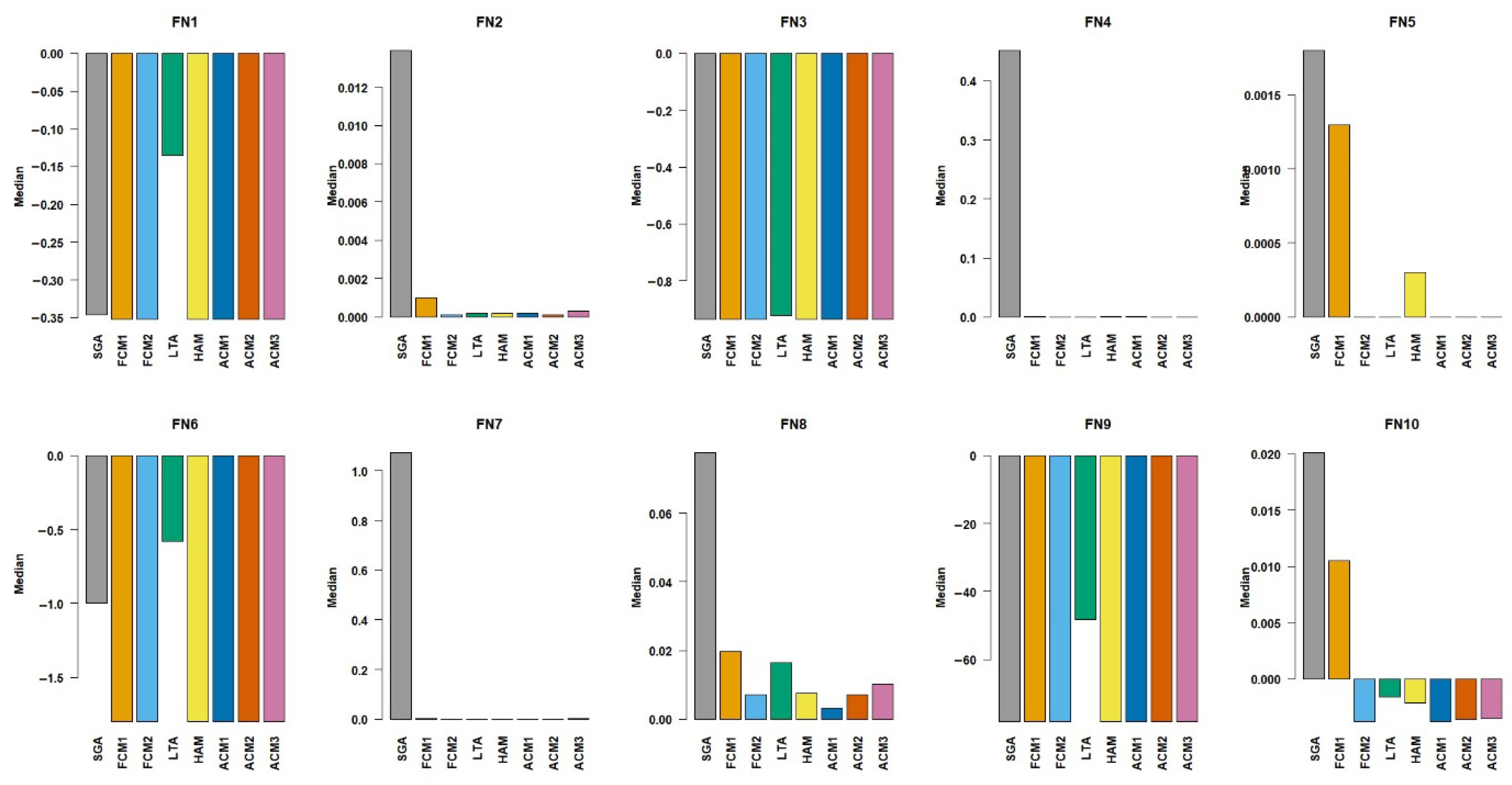
Different letters ond the median values indicate statistically significant different groups of methods (p ≤ 0.05).

presents the descriptive statistics of optimal solutions and statistical test results of the GAs for a population size of 20 ($n=20$). The median values of the optimal solutions are illustrated in Figure 3. The results show that FCM1, FCM2, HAM, ACM1, ACM2, and ACM3 converged to the global optimum value of approximately −0.3524 for the test function, FN1. SGA deviated from the optimum slightly, with a median value of −0.3463 and produced a relatively larger standard deviation of 0.0776, which hints that it is less stable than the other methods. Despite the FN1’s less complex structure, LTA underperformed, with a median value of −0.1356, having difficulty converging to the global optimum. For FN2, the methods FCM2, HAM, ACM1, ACM2, and ACM3 had near-zero errors and were in close approximation of the known global minimum. SGA and FCM1 produced relatively higher median values, implying less efficiency when handling the non-separable structure of FN2. In the tests with FN3, the methods FCM1, FCM2, HAM, ACM1, ACM2, and ACM3 returned results that were identical and close to the global optimum, −1. LTA showed a visible performance gap, with a median value of −0.9234 compared to the global optimum, indicating a bit lesser capability in handling steep gradient changes. For FN4, SGA recorded a substantially high median value of 0.4513 and a large variance, reflecting poor performance and instability. On the other hand, the methods FCM1, FCM2, HAM, ACM1, ACM2, and ACM3 could find solutions with negligible deviations from the global optimum, proving superior in global search and local refinement in a multimodal structure. For the FN5, the methods FCM2, LTA, HAM, ACM1, ACM2, and ACM3 found the global optimum. SGA’s median value of 0.0018 was slightly above the optimum, suggesting minor inefficiencies, while FCM1 also showed small but visible deviations. As for the FN6, the FCM1, FCM2, HAM, ACM1, ACM2, and ACM3 located the global optimum of approximately −1.8013. Meanwhile, LTA did not perform well with the median value of −0.5813, and SGA underperformed with −1.000, struggling to navigate the rugged search space. For FN7, the methods FCM2, HAM, ACM1, ACM2, and ACM3 deviated very slightly from the global optimum, expressing fine exploitation abilities. SGA, however, produced a higher median of 1.0723 and a large standard deviation of 1.2864, showing less performance. On FN8, the best-performing methods were FCM2, ACM1, and ACM2, producing median values that were close to the global optimum of 0. SGA, FCM1, and HAM had slightly higher median deviations, facing some difficulties in fine-tuning solutions along the curved valley towards the optimum. For FN9, except LTA, all the methods managed to locate the global optimum −78.3323, whereas LTA performed significantly worse because of premature convergences to locate the deepest minima. For FN10, the methods FCM2, HAM, ACM1, ACM2, and ACM3 found the global optimum. SGA and LTA deviated a bit from the optimum, hinting at minor inefficiencies in convergence.

The NCGOs and ranks of the compared methods are given in

Table 6. NCGO ranking of the methods for n = 20.

FN#		SGA	FCM1	FCM2	LTA	HAM	ACM1	ACM2	ACM3
FN1	NCGO	5	30	30	0	30	30	30	30
	Rank	7	3.5	3.5	8	3.5	3.5	3.5	3.5
FN2	NCGO	3	15	25	24	26	29	24	24
	Rank	8	7	3	5	2	1	5	5
FN3	NCGO	0	1	6	0	3	4	3	1
	Rank	7.5	5.5	1	7.5	3.5	2	3.5	5.5
FN4	NCGO	0	13	22	21	15	18	22	23
	Rank	8	7	1.5	3.5	6	5	1.5	3.5
FN5	NCGO	9	12	29	26	26	28	30	27
	Rank	8	7	2	5.5	5.5	3	1	4
FN6	NCGO	0	29	30	0	28	28	28	26
	Rank	7.5	2	1	7.5	4	4	4	6
FN7	NCGO	0	10	23	23	17	17	18	14
	Rank	8	7	1.5	1.5	4.5	4.5	3	6
FN8	NCGO	1	4	8	8	9	6	6	9
	Rank	8	7	3.5	3.5	1.5	5.5	5.5	1.5
FN9	NCGO	3	30	30	0	29	29	30	30
	Rank	7	2.5	2.5	8	5.5	5.5	2.5	2.5
FN10	NCGO	1	2	25	4	15	23	20	20
	Rank	8	7	1	6	5	2	3.5	3.5
	ΣRank	77	55.5	20.5	56	41	36	33	35

for $n=20$. Based on the NCGO results in Table 6, the methods FCM2, HAM, ACM1, ACM2, and ACM3 displayed a highly satisfactory performance, often attaining the maximum possible NCGO values for some functions such as FN1, FN6, and FN9. They maintained high rankings in both unimodal and multimodal problems, as well as the difficult non-separable cases like FN2, FN4, and FN8. Among these methods, the FCM2’s performance stood out, as it achieved top positions frequently. Throughout the test functions, FCM2 also achieved the lowest rank sum of 20.5. This was an unexpected superiority from the perspectives of this study, but it is worth mentioning that Hassanat et al. [25] had also reported that FCM2 configuration performs exceptionally better with small population sizes. On the FCM2’s performance in small population sizes (e.g., $n=20$), the fixed and relatively high mutation rate ($pm=0.5$) has a critical part. Genetic diversity tends to diminish rapidly in small populations and this may lead to premature convergence. Thus, the high mutation rate in FCM2 can be a countermeasure since it maintains the diversity. The balanced crossover rate of ($pc=0.5$) acts as complementary by ensuring steady exploitation without overwhelming the search with convergence pressure. As a result, the fixed but balanced setup of FCM2 seems to be effective especially under limited population diversity.

ACM1, ACM2, and ACM3 also performed very well with rank sums of 33, 35, and 36, respectively. HAM had a rank sum of 41, showing moderate performance due to a zero-mutation rate in early generations. SGA and LTA returned weaker results, frequently producing zero NCGOs for complex multimodal functions such as FN3, FN6, and FN9. Although the SGA achieved moderate success in FN1 and FN5, its performance remained consistently lower than that of the leading methods. LTA occasionally attained mid-tier rankings, as in FN2, FN4, and FN7, but these instances can be considered as exceptions rather than a consistent pattern. Overall, the integration of NCGO-based rankings and rank sums clearly confirms that FCM2 is the most successful and surprisingly dominant method for the given benchmark set with $n=20$, followed closely by ACM2, ACM1, and ACM3.

Table 7. Descriptive statistics of the optimal solutions for n = 50.

		Parameter Tuning and Control Methods
FN#	Stats	SGA	FCM1	FCM2	LTA	HAM	ACM1	ACM2	ACM3
FN1	Best	−0.3523	−0.3524	−0.3524	−0.1523	−0.3524	−0.3524	−0.3524	−0.3524
	Worst	−0.3524	−0.3524	−0.3524	−0.1253	−0.3524	−0.3524	−0.3523	−0.3524
	Median	−0.3506 b	−0.3524 a	−0.3524 a	−0.1481 c	−0.3524 a	−0.3524 a	−0.3524 a	−0.3524 a
	Mean	−0.3417	−0.3524	−0.3524	−0.1461	−0.3524	−0.3524	−0.3524	−0.3524
	Std.Dev.	0.0369	0.0000	0.0000	0.0062	0.0000	0.0000	0.0000	0.0000
FN2	Best	0.0000	0.0000	0.0000	0.0000	0.0000	0.0000	0.0000	0.0000
	Worst	0.1068	0.0049	0.0003	0.0016	0.0002	0.0004	0.0015	0.0007
	Median	0.0056 b	0.0000 a	0.0000 a	0.0000 a	0.0000 a	0.0000 a	0.0000 a	0.0000 a
	Mean	0.0103	0.0003	0.0000	0.0002	0.0000	0.0001	0.0001	0.0001
	Std.Dev.	0.0193	0.0009	0.0001	0.0003	0.0000	0.0001	0.0003	0.0002
FN3	Best	−0.9978	−1.0000	−1.0000	−0.9904	−1.0000	−1.0000	−1.0000	−1.0000
	Worst	−0.9358	−0.9362	−0.9362	−0.9215	−0.9362	−0.9362	−0.9362	−0.9362
	Median	−0.9362 a	−0.9362 a	−0.9362 a	−0.9347 b	−0.9362 a	−0.9362 a	−0.9362 a	−0.9362 a
	Mean	−0.9400	−0.9426	−0.9659	−0.9358	−0.9405	−0.9575	−0.9532	−0.9532
	Std.Dev.	0.0145	0.0194	0.0322	0.0141	0.0161	0.0305	0.0287	0.0286
FN4	Best	0.0001	0.0000	0.0000	0.0000	0.0000	0.0000	0.0000	0.0000
	Worst	5.9547	0.0075	0.0009	0.0029	0.0041	0.0033	0.0119	0.0214
	Median	0.0230 b	0.0002 a	0.0001 a	0.0001 a	0.0000 a	0.0000 a	0.0000 a	0.0000 a
	Mean	0.3239	0.0011	0.0001	0.0002	0.0004	0.0003	0.0008	0.0011
	Std.Dev.	1.0894	0.0018	0.0002	0.0006	0.0010	0.0006	0.0027	0.0039
FN5	Best	0.0031	0.0011	0.0000	0.0000	0.0001	0.0000	0.0000	0.0000
	Worst	0.0000	0.0000	0.0000	0.0000	0.0000	0.0000	0.0000	0.0000
	Median	0.0006 b	0.0001 a	0.0000 a	0.0000 a	0.0000 a	0.0000 a	0.0000 a	0.0000 a
	Mean	0.0008	0.0002	0.0000	0.0000	0.0000	0.0000	0.0000	0.0000
	Std.Dev.	0.0008	0.0003	0.0000	0.0000	0.0000	0.0000	0.0000	0.0000
FN6	Best	−1.8013	−1.8013	−1.8013	−1.1662	−1.8013	−1.8013	−1.8013	−1.8013
	Worst	−0.8778	−1.8008	−1.8011	0.0000	−1.0597	−1.8013	−1.8013	−1.8012
	Median	−1.0929 b	−1.8013 a	−1.8013 a	−0.7994c	−1.8013 a	−1.8013 a	−1.8013 a	−1.8013 a
	Mean	−1.3127	−1.8013	−1.8013	−0.6809	−1.7731	−1.8013	−1.8013	−1.8013
	Std.Dev.	0.3668	0.0001	0.0000	0.3275	0.1355	0.0000	0.0000	0.0000
FN7	Best	0.0118	0.0000	0.0000	0.0000	0.0000	0.0000	0.0000	0.0000
	Worst	1.0804	0.0064	0.0039	0.0010	0.9951	0.9950	0.9956	0.9953
	Median	0.2228 b	0.0001 a	0.0001 a	0.0001 a	0.0001 a	0.0002 a	0.0002 a	0.0001 a
	Mean	0.4536	0.0010	0.0003	0.0002	0.0335	0.0667	0.0668	0.0997
	Std.Dev.	0.4503	0.0018	0.0007	0.0003	0.1816	0.2523	0.2525	0.3036
FN8	Best	0.0016	0.0004	0.0000	0.0000	0.0000	0.0000	0.0001	0.0000
	Worst	0.2515	0.1248	0.0478	0.0819	0.0763	0.0441	0.0593	0.0290
	Median	0.0353 d	0.0067 c	0.0034 bc	0.0021 b	0.0027 b	0.0013 a	0.0021 b	0.0013 a
	Mean	0.0515	0.0181	0.0076	0.0087	0.0088	0.0068	0.0095	0.0044
	Std.Dev.	0.0573	0.0286	0.0110	0.0174	0.0158	0.0113	0.0148	0.0066
FN9	Best	−78.3323	−78.3323	−78.3323	−75.9838	−78.3323	−78.3323	−78.3323	−78.3323
	Worst	−64.1716	−78.3322	−78.3323	−36.9894	−78.3323	−78.3323	−78.3321	−78.3321
	Median	−78.3300 a	−78.3323 a	−78.3323 a	−61.1664 b	−78.3323 a	−78.3323 a	−78.3323 a	−78.3323 a
	Mean	−77.3634	−78.3323	−78.3323	−59.4596	−78.3323	−78.3323	−78.3323	−78.3323
	Std.Dev.	3.5840	0.0000	0.0000	11.7644	0.0000	0.0000	0.0000	0.0000
FN10	Best	−0.0037	−0.0038	−0.0038	−0.0038	−0.0038	−0.0038	−0.0038	−0.0038
	Worst	0.0363	0.0017	−0.0037	−0.0005	−0.0037	−0.0035	−0.0032	−0.0038
	Median	0.0052 c	−0.0035 b	−0.0038 b	−0.0022 a	−0.0038 b	−0.0038 b	−0.0038 b	−0.0038 b
	Mean	0.0085	−0.0031	−0.0038	−0.0023	−0.0038	−0.0038	−0.0038	−0.0038
	Std.Dev.	0.0116	0.0011	0.0000	0.0010	0.0000	0.0000	0.0001	0.0000

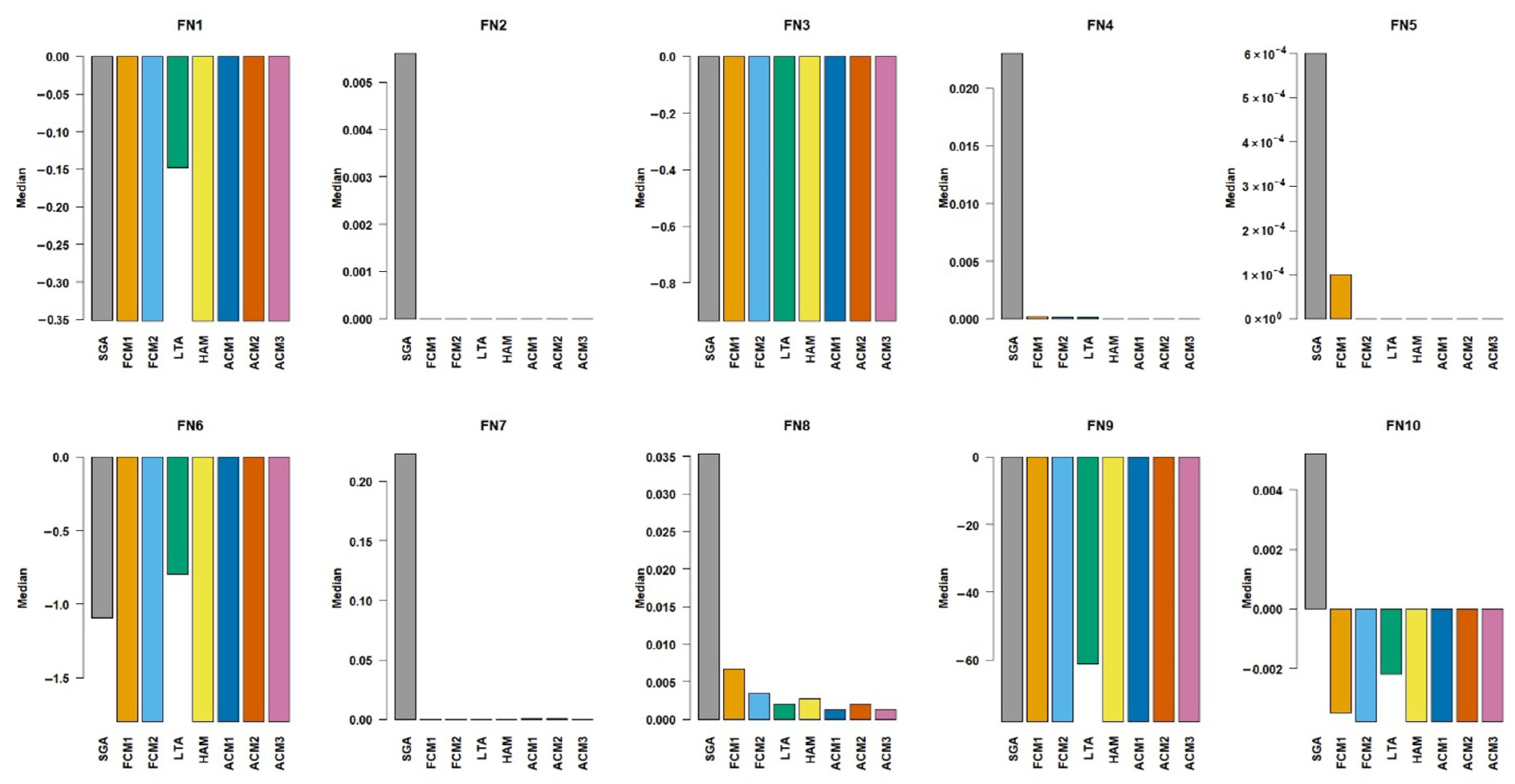
Different letters indicate statistically significant different groups of methods (p ≤ 0.05).

presents the descriptive statistics and statistical comparisons of the optimal solutions obtained from different parameter tunings and control methods for a population size of 50 ($n=50$). As also illustrated in Figure 4, the methods FCM1, FCM2, HAM, ACM1, ACM2, and ACM3 successfully converged to the global optimum of approximately −0.3524 for the FN1 test function. Meanwhile, SGA produced a median of −0.3506 close to the global optimum, LTA performed considerably worse, with a median of −0.1481, suggesting it struggled to locate the optimum despite the simplicity of the FN1 function. On FN2, all the methods except SGA have been very successful by achieving a median of exactly 0, which is the global optimum. SGA yielded a larger median of 0.0056 for FN2. Regarding the function FN3, the medians of all methods have been found as very close to the global optimum of −1, while LTA had a slightly higher median of −0.9347. In FN4, however, the methods HAM, ACM1, ACM2, and ACM3 had the medians equal to the global optimum; there were no significant differences with FCM1, FCM2, and LTA, also implying their capability in multimodal optimisation. For this function, even though SGA’s median is a bit higher than the optimum it found the best results close to the global optimum. For FN5, the methods FCM2, LTA, HAM, ACM1, ACM2, and ACM3 reached the global optimum. SGA produced a slightly higher median of 0.0006. On FN6, the methods FCM1, FCM2, HAM, ACM1, ACM2, and ACM3 perfectly found the optimum value. SGA’s median of −1.0929 indicates weaker performance, while LTA’s result of −0.7994 reflects significant difficulty in navigating the rugged search space. For FN7, the methods FCM1, FCM2, LTA, HAM, ACM1, ACM2, and ACM3 achieved medians very close to zero, showing effective exploitation ability. For FN8, although ACM1 and ACM3 gave the media results very close to the global optimum, LTA, HAM, and ACM2 also approached the global optimum, pointing to their efficient fine-tuning capability. SGA and FCM1 performed slightly worse, suggesting they were less precise in handling the curved search space of FN8. On FN9, all methods but SGA and LTA perfectly achieved the global optimum. SGA’s median was quite close, but it was less stable due to larger standard deviations of solutions, whereas LTA’s median indicates premature convergence and a significant amount of divergence. Lastly, for FN10, FCM1, FCM2, HAM, ACM1, ACM2, and ACM3 did not differ in median performance. SGA and LTA exhibited small but consistent deviations, reflecting slight inefficiencies in convergence accuracy.

Table 8. NCGO ranking of the methods for n = 50.

FN#		SGA	FCM1	FCM2	LTA	HAM	ACM1	ACM2	ACM3
FN1	NCGO	11	30	30	0	30	30	30	30
	Rank	7	3.5	3.5	8	3.5	3.5	3.5	3.5
FN2	NCGO	7	28	30	29	30	30	29	30
	Rank	8	7	2.5	5.5	2.5	2.5	5.5	2.5
FN3	NCGO	0	3	13	0	2	10	8	8
	Rank	7.5	5	1	7.5	6	2	3.5	3.5
FN4	NCGO	1	20	30	28	27	28	27	25
	Rank	8	7	1	2.5	4.5	2.5	4.5	6
FN5	NCGO	21	29	30	30	30	30	30	30
	Rank	8	7	3.5	3.5	3.5	3.5	3.5	3.5
FN6	NCGO	3	30	30	0	26	30	30	30
	Rank	7	3	3	8	6	3	3	3
FN7	NCGO	0	25	28	30	27	25	23	27
	Rank	8	5.5	2	1	3.5	5.5	7	3.5
FN8	NCGO	0	6	9	11	9	13	11	15
	Rank	8	7	5.5	3.5	5.5	2	3.5	1
FN9	NCGO	11	30	30	0	30	30	30	30
	Rank	7	3.5	3.5	8	3.5	3.5	3.5	3.5
FN10	NCGO	2	23	30	11	30	30	30	30
	Rank	8	6	3	7	3	3	3	3
	ΣRank	76.5	54.5	28.5	54.5	41.5	31.0	40.5	33.0

presents a summary of the performance of methods across test functions, focusing on NCGOs and their corresponding ranks. The table also includes the rank sums for overall performance. As seen in the table, FCM2 emerged as the best-performing method with the lowest rank sum and perfect NCGO scores for six functions of FN2, FN4, FN5, FN6, FN9, and FN10, confirming its superiority. Among the stronger performers, ACM1 and ACM3 came closest to FCM2, while HAM and ACM2 showed good results, particularly on FN3, FN4, FN7, and FN8. FCM1 performed well on some functions, such as FN1, FN2, FN6, and FN9, but poorly on others, indicating problem-specific sensitivity. SGA was the weakest with the highest rank sum of 76.5, and failing entirely on FN3, FN7, and FN8 with zero NCGOs. LTA matched FCM1 in rank but was highly inconsistent, with zero NCGOs for FN1, FN3, FN6, and FN9.

Table 9. Descriptive statistics of the optimal solutions for n = 100.

FN#	Stats	SGA	FCM1	FCM2	LTA	HAM	ACM1	ACM2	ACM3
FN1	Best	−0.3524	−0.3524	−0.3524	−0.1526	−0.3524	−0.3524	−0.3524	−0.3524
	Worst	−0.3490	−0.3524	−0.3524	−0.1388	−0.3524	−0.3524	−0.3524	−0.3524
	Median	−0.3523 a	−0.3524 a	−0.3524 a	−0.1509 c	−0.3524 a	−0.3524 a	−0.3524 a	−0.3524 a
	Mean	−0.3520	−0.3524	−0.3524	−0.1496	−0.3524	−0.3524	−0.3524	−0.3524
	Std.Dev.	0.0008	0.0000	0.0000	0.0035	0.0000	0.0000	0.0000	0.0000
FN2	Best	0.0000	0.0000	0.0000	0.0000	0.0000	0.0000	0.0000	0.0000
	Worst	0.0427	0.0023	0.0003	0.0002	0.0003	0.0002	0.0002	0.0003
	Median	0.0001 a	0.0000 a	0.0000 a	0.0000 a	0.0000 a	0.0000 a	0.0000 a	0.0000 a
	Mean	0.0044	0.0001	0.0000	0.0000	0.0000	0.0000	0.0000	0.0000
	Std.Dev.	0.0084	0.0004	0.0001	0.0001	0.0001	0.0000	0.0000	0.0001
FN3	Best	−0.9964	−1.0000	−1.0000	−0.9904	−1.0000	−1.0000	−1.0000	−1.0000
	Worst	−0.9360	−0.9362	−0.9362	−0.9235	−0.9362	−0.9362	−0.9362	−0.9362
	Median	−0.9362 c	−0.9362 b	−0.9999 a	−0.9359 c	−0.9362 b	−0.9999 a	−0.9996 a	−0.9362 b
	Mean	−0.9422	−0.9575	−0.9893	−0.9382	−0.9615	−0.9868	−0.9702	−0.9617
	Std.Dev.	0.0182	0.0306	0.0241	0.0131	0.0315	0.0258	0.0323	0.0317
FN4	Best	0.0000	0.0000	0.0000	0.0000	0.0000	0.0000	0.0000	0.0000
	Worst	0.3066	0.0061	0.0003	0.0002	0.0005	0.0004	0.0009	0.0011
	Median	0.0078 b	0.0000 a	0.0000 a	0.0000 a	0.0000 a	0.0000 a	0.0000 a	0.0000 a
	Mean	0.0480	0.0006	0.0001	0.0000	0.0001	0.0001	0.0001	0.0001
	Std.Dev.	0.0814	0.0016	0.0001	0.0000	0.0001	0.0001	0.0002	0.0002
FN5	Best	0.0000	0.0000	0.0000	0.0000	0.0000	0.0000	0.0000	0.0000
	Worst	0.0017	0.0001	0.0000	0.0000	0.0000	0.0000	0.0000	0.0000
	Median	0.0003 b	0.0000 a	0.0000 a	0.0000 a	0.0000 a	0.0000 a	0.0000 a	0.0000 a
	Mean	0.0004	0.0000	0.0000	0.0000	0.0000	0.0000	0.0000	0.0000
	Std.Dev.	0.0004	0.0000	0.0000	0.0000	0.0000	0.0000	0.0000	0.0000
FN6	Best	−1.8013	−1.8013	−1.8013	−1.8013	−1.8013	−1.8013	−1.8013	−1.8013
	Worst	−1.7795	−1.8013	−1.8013	−0.3323	−1.2854	−1.8013	−1.8013	−1.8013
	Median	−1.4421 c	−1.8013 a	−1.8013 a	−1.7961 b	−1.8013 a	−1.8013 a	−1.8013 a	−1.8013 a
	Mean	−1.4091	−1.8013	−1.8013	−1.0175	−1.7795	−1.8013	−1.8013	−1.8013
	Std.Dev.	0.3707	0.0000	0.0000	0.2866	0.0967	0.0000	0.0000	0.0000
FN7	Best	0.0000	0.0000	0.0000	0.0000	0.0000	0.0000	0.0000	0.0000
	Worst	1.0595	0.0009	0.0006	0.0009	0.0008	0.0010	0.0005	0.0016
	Median	0.0339 b	0.0001 a	0.0001 a	0.0000 a	0.0001 a	0.0001 a	0.0001 a	0.0001 a
	Mean	0.2427	0.0002	0.0002	0.0001	0.0001	0.0002	0.0001	0.0002
	Std.Dev.	0.3999	0.0002	0.0002	0.0002	0.0002	0.0002	0.0001	0.0003
FN8	Best	0.0009	0.0000	0.0000	0.0000	0.0001	0.0000	0.0000	0.0000
	Worst	0.1851	0.0277	0.0116	0.0212	0.0103	0.0362	0.0158	0.0359
	Median	0.0170 c	0.0012 b	0.0007 a	0.0016 c	0.0006 a	0.0010 b	0.0015 bc	0.0011 b
	Mean	0.0326	0.0046	0.0021	0.0032	0.0015	0.0028	0.0034	0.0039
	Std.Dev.	0.0009	0.0000	0.0000	0.0000	0.0001	0.0000	0.0000	0.0000
FN9	Best	−78.3323	−78.3323	−78.3323	−78.3198	−78.3323	−78.3323	−78.3323	−78.3323
	Worst	−78.3196	−78.3322	−78.3323	−60.9626	−78.3323	−78.3323	−78.3323	−78.3323
	Median	−78.3319 a	−78.3323 a	−78.3323 a	−75.9837 b	−78.3323 a	−78.3323 a	−78.3323 a	−78.3323 a
	Mean	−78.3312	−78.3323	−78.3323	−74.4364	−78.3323	−78.3323	−78.3323	−78.3323
	Std.Dev.	0.0024	0.0000	0.0000	4.4622	0.0000	0.0000	0.0000	0.0000
FN10	Best	−0.0038	−0.0038	−0.0038	−0.0038	−0.0038	−0.0038	−0.0038	−0.0038
	Worst	0.0210	−0.0034	−0.0038	−0.0003	−0.0038	−0.0038	−0.0038	−0.0038
	Median	−0.0024 a	−0.0038 b	−0.0038 b	−0.0023 a	−0.0038 b	−0.0038 b	−0.0038 b	−0.0038 b
	Mean	−0.0035	−0.0038	−0.0038	−0.0021	−0.0038	−0.0038	−0.0038	−0.0038
	Std.Dev.	0.0056	0.0001	0.0000	0.0012	0.0000	0.0000	0.0000	0.0000

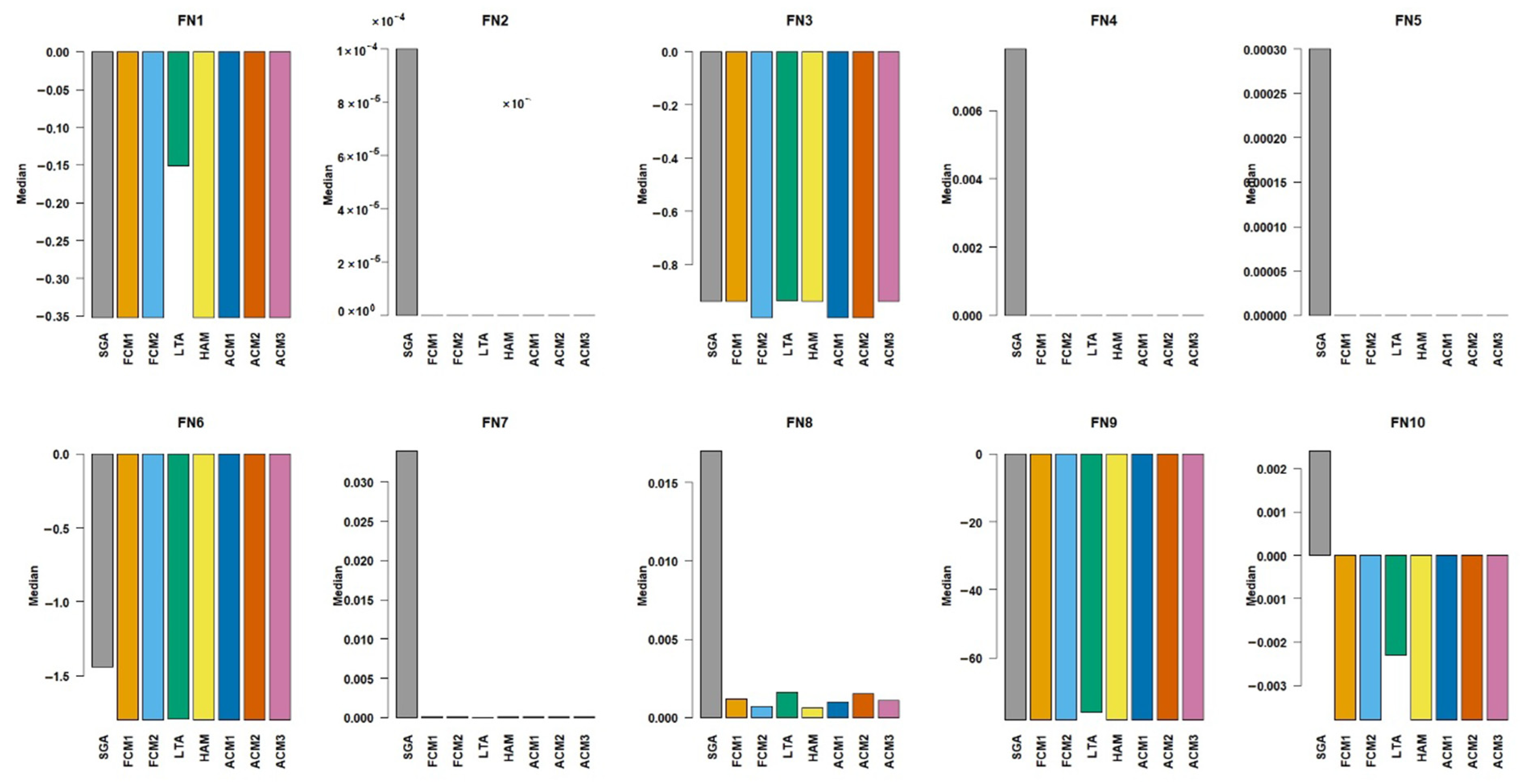
Different letters indicate statistically significant different groups of methods (p ≤ 0.05).

lists the descriptive statistics for the optimal solutions found for a larger population size of $n=100$. As shown in Table 9 and as the median values in Figure 5 display, the methods FCM1, FCM2, HAM, ACM1, ACM2, and ACM3 achieved excellent results across almost all of the functions. For FN1, FN2, FN4, FN5, FN6, FN9, and FN10, these methods either matched up or were only negligibly different from the global optimum, as indicated by their median values. Their standard deviations were often zero or close to it, showing a remarkable stability and reliability in finding the optimal solution in larger populations.

SGA method, in general, performed worse than the other methods. For example, in FN1, FN2, and FN5, SGA’s median was statistically different from the more successful methods, and its standard deviation was notably higher, suggesting less consistent convergence. However, when considered on its own, it showed a little improvement for the larger population size $n=100$ compared to that of the previous test, where $n=50$.

LTA showed a mixed performance. It struggled heavily with certain functions, such as FN1 and FN9, where its median values fell far from the global optimum. For FN9, the standard deviation was 4.4622, indicating a huge variability in its results. However, it performed well on functions like FN4 and FN7, achieving pristine medians of 0.0000 and 0.0000, respectively, statistically on par with the best methods. We may therefore conclude that the LTA’s effectiveness is highly dependent on the characteristics of the optimisation problem, such as population size.

According to the results in

Table 10. NCGO ranking of the methods for n = 100.

FN#		SGA	FCM1	FCM2	LTA	HAM	ACM1	ACM2	ACM3
FN1	NCGO	25	30	30	0	30	30	30	30
	Rank	7	3.5	3.5	8	3.5	3.5	3.5	3.5
FN2	NCGO	15	29	30	30	30	30	30	30
	Rank	8	7	3.5	3.5	3.5	3.5	3.5	3.5
FN3	NCGO	0	10	25	0	11	23	16	12
	Rank	7.5	6	1	7.5	5	2	3	4
FN4	NCGO	3	27	30	30	30	30	30	29
	Rank	8	7	3	3	3	3	3	6
FN5	NCGO	27	30	30	30	30	30	30	30
	Rank	8	4	4	4	4	4	4	4
FN6	NCGO	10	30	30	0	28	30	30	30
	Rank	7	3	3	8	6	3	3	3
FN7	NCGO	7	30	30	30	30	29	30	29
	Rank	8	3	3	3	3	6.5	3	6.5
FN8	NCGO	1	14	18	13	20	15	13	14
	Rank	8	4.5	2	6.5	1	3	6.5	4.5
FN9	NCGO	21	30	30	0	30	30	30	30
	Rank	7	3.5	3.5	8	3.5	3.5	3.5	3.5
FN10	NCGO	3	30	30	10	30	30	30	30
	Rank	8	3.5	3.5	7	3.5	3.5	3.5	3.5
	ΣRank	76.5	45.0	30.0	58.5	36.0	35.5	36.5	42.0

, FCM2 is the best-performing method with the lowest rank sum of 30.0. It achieved an impressive NCGO score of 30 on many functions, including FN2, FN4, FN5, FN6, FN7, FN9, and FN10, an indicator of its ability to converge to the global optimum across a variety of problem types. There was a slight dip in performance on FN3 and FN8, but it still managed to reserve the ranks of 1 and 2, respectively. The methods ACM1, HAM, and ACM2 also performed very well, with rank sum values of 35.5, 36.0, and 36.5, respectively. These scores indicate high performance, nearly matching that of the FCM2. The trio achieved NCGO scores of 30 with most functions, showing significant consistency. Compared to the FCM2’s performance, the most visible differences were observed for FN3 and FN8, where their NCGO values were a bit lower, which suggests a minor but not statistically significant difference in their fine-tuning capabilities. In the third group, the methods FCM1 and ACM3 showed a decent overall performance with rank sums of 45.0 and 42.0, respectively. FCM1 consistently located the global optimum on functions like FN1, FN2, FN5, FN7, FN9, and FN10. However, its performance fell dramatically on FN3 and FN8, where its NCGO values decreased to 10 and 14, respectively. This inconsistency suggests that although FCM1 is highly effective, it may struggle with certain complex function landscapes. ACM3 followed a similar pattern, with satisfactory performance on most functions while scoring a lower NCGO on FN3 and FN8. The LTA and SGA methods were the weakest performers. LTA has a quite large rank sum of 58.5, and its performance is highly inconsistent. It totally failed on functions like FN1, FN3, and FN9, demonstrating a clear weakness to specific types of optimisation problems. In contrast, though, the LTA’s performances on FN2, FN4, FN5, and FN7 were perfect, which suggests a significant dependency on the function’s characteristics. SGA showed the worst performance, with a very large rank sum of 76.5. Its NCGO values were consistently low across the methods, and it failed to find the optimum in any run for FN3, confirming its ineffectiveness for more challenging problems, even with an increased population size.

4.2. Results from Experiment 2

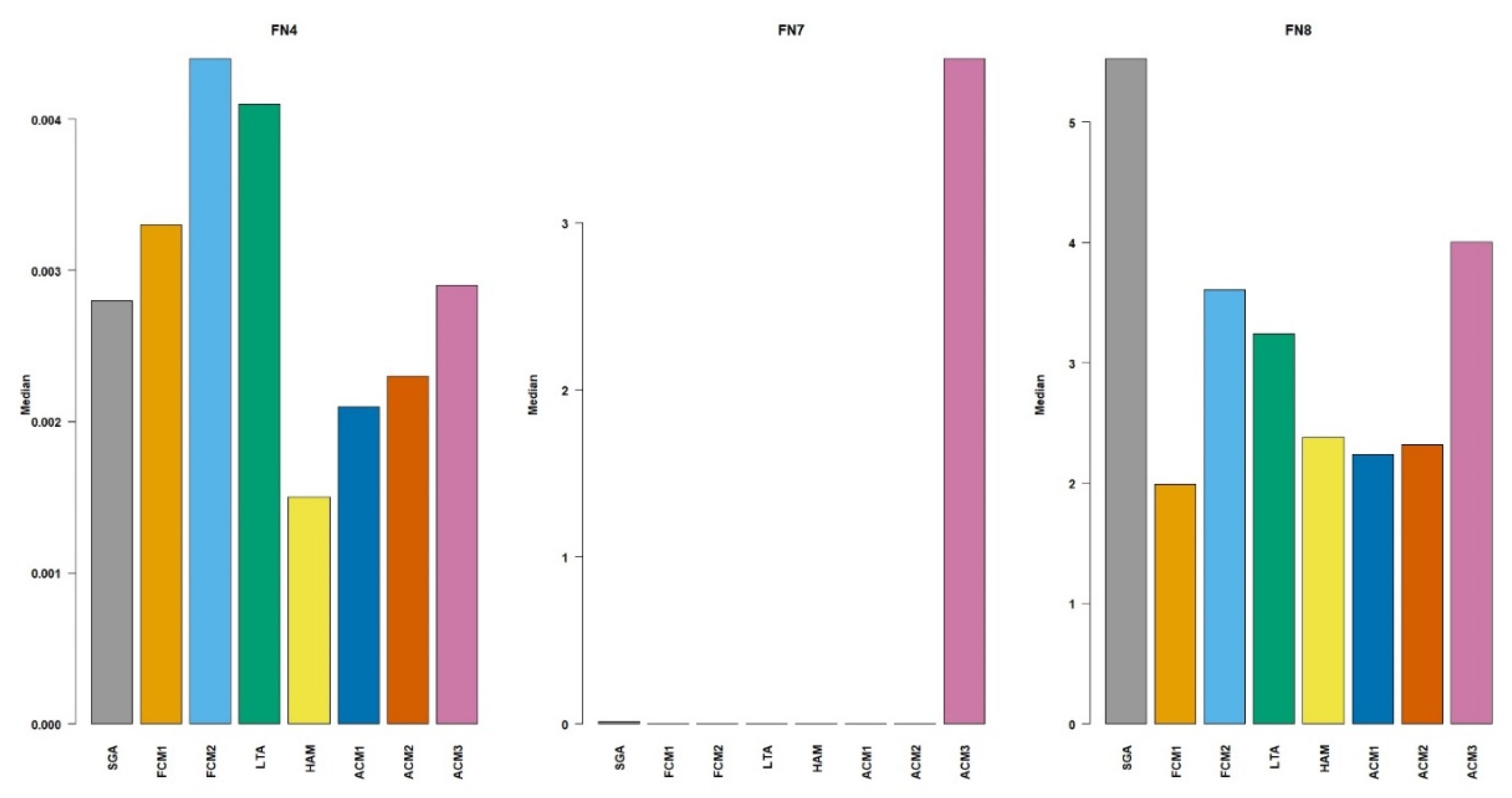
Experiment 2 begins with the settings, $d=5$, $n=250$, and, $g_{max}=100$. According to the results presented in

Table 11. Descriptive statistics of the optimal solutions for d = 5 and n = 250, g_max = 100.

FN#	Stats	SGA	FCM1	FCM2	LTA	HAM	ACM1	ACM2	ACM3
FN4	Best	0.0072	0.0001	0.0002	0.0001	0.0001	0.0001	0.0001	0.0003
	Worst	0.5422	0.0689	0.0059	0.0104	0.0443	0.0186	0.0089	0.0142
	Median	0.0491 c	0.0016 a	0.0013 a	0.0021 ab	0.0015 a	0.0021 ab	0.0013 a	0.0022 ab
	Mean	0.1067	0.0065	0.0019	0.0029	0.0034	0.0039	0.0021	0.0030
	Std.Dev.	0.1392	0.0138	0.0017	0.0027	0.0080	0.0043	0.0024	0.0030
FN7	Best	0.0114	0.0002	0.0004	0.0005	0.0003	0.0005	0.0003	0.0013
	Worst	2.0222	1.0041	1.0065	1.0234	1.0007	0.9989	0.9978	1.0031
	Median	1.0322 c	0.0056 ab	0.0063 ab	0.0071 ab	0.0033 a	0.0038 a	0.0062 ab	0.0068 ab
	Mean	0.8873	0.0735	0.2046	0.1419	0.0703	0.0709	0.1047	0.1069
	Std.Dev.	0.6327	0.2521	0.4045	0.3486	0.2524	0.2522	0.3024	0.3030
FN8	Best	0.0008	0.0008	0.0002	0.0011	0.0001	0.0002	0.0000	0.0033
	Worst	1.3381	0.7677	0.3783	0.4451	0.3570	0.3657	0.5100	0.3528
	Median	0.2485 c	0.1939 b	0.0726 a	0.0893 a	0.0873 a	0.0981 a	0.1076 ab	0.0899 a
	Mean	0.3714	0.2771	0.0957	0.1214	0.0907	0.1184	0.1208	0.1058
	Std.Dev.	0.3333	0.2362	0.0912	0.1105	0.0759	0.0912	0.1021	0.0841

Different letters indicate statistically significant different groups of methods (p ≤ 0.05).

and Figure 6, the SGA performed the worst in general. For the FN4 function, SGA with a median of 0.0491 performed significantly worse than all the other methods. The remaining methods showed no statistically significant difference in median performance, ranging from 0.0013 to 0.0022. On the FN7 function, the SGA again stands out with a significantly higher median value. The methods HAM and ACM1 were statistically similar and the best-performing group. The methods FCM1, FCM2, LTA, ACM2, and ACM3 performed similarly to each other. For the FN8 function, the analysis of median values again shows that SGA performed significantly worse than all other methods. The methods FCM2, LTA, HAM, ACM1, ACM2, and ACM3 gave statistically similar results.

According to the NCGOs and ranks given in

Table 12. NCGO ranking of the methods for d = 5 and n = 250, g_max = 100.

FN#		SGA	FCM1	FCM2	LTA	HAM	ACM1	ACM2	ACM3
FN4	NCGO	0	10	13	10	11	6	13	9
	Rank	8	4.5	1.5	4.5	3	7	1.5	6
FN7	NCGO	0	3	2	2	5	2	4	0
	Rank	7.5	3	5	5	1	5	2	7.5
FN8	NCGO	1	1	1	0	2	1	2	0
	Rank	5	5	5	8	1.5	5	1.5	5
	ΣRank	20.5	12.5	11.5	17.5	5.5	17	5	18.5

, the best method overall was the ACM2, followed by the HAM and FCM2.

The results for the configuration of $d=10$ and $n=500$ on the test functions are shown in

Table 13. Descriptive statistics of the optimal solutions for d = 10 and n = 500.

FN#	Stats	SGA	FCM1	FCM2	LTA	HAM	ACM1	ACM2	ACM3
FN4	Best	0.0026	0.0000	0.0001	0.0000	0.0001	0.0001	0.0001	0.0001
	Worst	2.0154	0.0014	0.9961	1.0119	0.0016	0.0028	0.9951	0.6672
	Median	0.0177 c	0.0009 ab	0.0006 b	0.0009 ab	0.0004 a	0.0007 b	0.0004 a	0.0008 b
	Mean	0.1174	0.0238	0.0080	0.0464	0.0231	0.0453	0.0005	0.0699
	Std.Dev.	0.2334	0.1214	0.0388	0.1695	0.1216	0.1690	0.0002	0.2028
FN7	Best	0.0005	0.0001	0.0001	0.0001	0.0002	0.0002	0.0002	0.0007
	Worst	2.0154	0.0014	0.3037	0.3812	0.0003	0.0005	0.9951	4.9755
	Median	0.0109 c	0.0000 a	0.0008 b	0.0005 ab	0.0005 ab	0.0007 b	0.0006 b	1.9905 d
	Mean	0.3099	0.0006	0.1003	0.1682	0.0006	0.0007	0.0338	1.9906
	Std.Dev.	0.5965	0.0004	0.3037	0.3812	0.0003	0.0005	0.1816	1.3064
FN8	Best	0.1489	0.0029	0.0521	0.0259	0.0495	0.0220	0.0234	0.0736
	Worst	8.0025	7.0099	6.7225	8.9203	7.4243	8.2999	6.5410	7.8109
	Median	3.2502 b	2.5290 a	2.7957 a	3.1751 b	2.5062 a	2.5017 a	2.4000 a	2.6263 a
	Mean	3.2390	2.5092	2.9587	3.2001	2.7228	2.9570	2.4289	2.8197
	Std.Dev.	2.0341	1.7679	1.9045	2.3752	1.8504	2.1432	1.7452	2.0807

Different letters indicate statistically significant different groups of methods (p ≤ 0.05).

and plotted in Figure 7. For the FN4 benchmark function, SGA performed statistically worse than all other methods, with a median value of 0.0177. The best performance was achieved by HAM and ACM2, with a median value of 0.0004 for both. These are followed by the methods FCM2, ACM1, and ACM3. On FN7, the performance results were more distinct. SGA and ACM3 performed significantly worse than the other methods. FCM1, with a median value of 0.0000, was the single best-performing method. The methods FCM2, ACM1, and ACM2 formed a statistically similar group, representing the second-best performers. LTA and HAM had an intermediate performance. For FN8, most of the methods exhibited a similar level of performance. Although ACM2 had the lowest median value, the methods FCM1, FCM2, HAM, ACM1, ACM2, and ACM3 belonged to a single, statistically similar group. This group collectively represents the best performance. In contrast, SGA and LTA performed worse than the methods.

According to the NCGO ranking results shown in

Table 14. NCGO ranking of the methods for d = 10 and n = 500.

FN#		SGA	FCM1	FCM2	LTA	HAM	ACM1	ACM2	ACM3
FN4	NCGO	0	16	25	15	24	21	28	20
	Rank	8	6	2	7	3	4	1	5
FN7	NCGO	2	25	18	20	27	24	27	3
	Rank	8	3	6	5	1.5	4	1.5	7
FN8	NCGO	0	0	0	0	0	0	0	0
	Rank	4.5	4.5	4.5	4.5	4.5	4.5	4.5	4.5
	ΣRank	20.5	13.5	8	16.5	9	12.5	7	11.5

, the best performance was scored by the ACM2, followed by the FCM2 and HAM, with the rank values of 7, 8, and 9, respectively.

The results for the configuration of $d=15$ and $n=750$ on the test functions are shown in

Table 15. Descriptive statistics of the optimal solutions for d = 15 and n = 750.

		Parameter Tuning and Control Methods
FN#	Stats	SGA	FCM1	FCM2	LTA	HAM	ACM1	ACM2	ACM3
FN4	Best	0.0080	0.0004	0.0004	0.0008	0.0006	0.0004	0.0004	0.0005
	Worst	1.4802	1.0032	1.1246	0.9955	0.0450	0.6742	0.8418	0.6671
	Median	0.0028 ab	0.0033 ab	0.0044 b	0.0041 b	0.0015 a	0.0021 ab	0.0023 ab	0.0029 ab
	Mean	0.1169	0.0380	0.1792	0.1764	0.0044	0.0500	0.0528	0.1805
	Std.Dev.	0.2875	0.1824	0.3216	0.3125	0.0086	0.1691	0.1921	0.2983
FN7	Best	0.0017	0.0004	0.0003	0.0005	0.0004	0.0006	0.0004	0.9958
	Worst	1.0030	0.9959	1.9914	1.0202	0.9963	0.0026	0.0026	7.9614
	Median	0.0151 b	0.0012 a	0.0017 b	0.0017 b	0.0012 a	0.0013 a	0.0013 a	3.9808 c
	Mean	0.2097	0.0675	0.2667	0.1700	0.0343	0.0013	0.0014	3.9481
	Std.Dev.	0.4019	0.2523	0.5181	0.3827	0.1817	0.0005	0.0005	1.6831
FN8	Best	0.2140	0.0284	0.0926	0.1144	0.0586	0.0709	0.0573	0.1159
	Worst	68.0557	64.6640	14.5262	65.9862	10.9691	59.4197	14.5699	14.0417
	Median	5.5254 d	1.9896 a	3.6097 bc	3.2395 bc	2.3837 b	2.2371 b	2.3195 b	4.0062 c
	Mean	11.8833	8.0345	4.9743	6.5973	3.6871	5.5778	4.2319	5.2443
	Std.Dev.	18.6821	17.0882	4.5405	11.9236	3.9196	10.9329	3.8005	4.3510

Different letters indicate statistically significant different groups of methods (p ≤ 0.05).

and

Table 16. NCGO ranking of the methods for d = 15 and n = 750.

FN#		SGA	FCM1	FCM2	LTA	HAM	ACM1	ACM2	ACM3
FN4	NCGO	0	5	4	2	6	6	9	3
	Rank	8	4	5	7	2.5	2.5	1	6
FN7	NCGO	0	9	8	5	12	7	7	0
	Rank	7.5	2	3	6	1	4.5	4.5	7.5
FN8	NCGO	0	0	0	0	0	0	0	0
	Rank	4.5	4.5	4.5	4.5	4.5	4.5	4.5	4.5
	ΣRank	20	10.5	12.5	17.5	8	11.5	10	18

, and they are plotted in Figure 8. For FN4, HAM demonstrated a statistically superior performance, outperforming the rest. A large group of methods, including SGA, FCM1, ACM1, ACM2, and ACM3, performed similarly to this top-tier method, with no significant differences among them. However, FCM2 and LTA showed a statistically worse performance compared to the best one. This indicates that while HAM was the standout performer, a large number of methods were also highly effective. The performance on FN7 was clearly divided into three distinct levels. The methods FCM1, HAM, ACM1, and ACM2 achieved the best results with the lowest median values, performing in a statistically similar manner. A second group, consisting of SGA, FCM2, and LTA, showed significantly worse results than the top performers. Finally, ACM3 had a median so high that it was statistically worse than all other methods. On the FN8 function, FCM1 was statistically the best, surpassing all others. The group of HAM, ACM1, and ACM2 performed worse than FCM1 but were still more effective than the rest. FCM2 and LTA showed an intermediate level of performance, while SGA had the worst performance of all, with a median value that was statistically higher than every other method.

According to the NCGOs in Table 16, the ACM2 was the best method, followed by the HAM and ACM1, on the test function FN4, while the HAM was the best, followed by FCM1 and FCM2, on the test function FN7. On the other hand, the ACM1 and ACM2 also performed well on this function, as seen in Figure 8. Finally, on the test function FN8 (Rosenbrock), all of the methods had the same rank score. Picheny et al. [52] reported that, even though the valley of the Rosenbrock function is easy to find, convergence to the global minimum is very difficult for the larger dimensions with it. The zero NCGO values observed for the Rosenbrock function in Table 16 also suggested a substantial difficulty for all of the compared algorithms in locating the global optimum. Although the Rosenbrock function has a narrow valley guiding toward the global minimum, its curvature becomes highly non-linear and poorly conditioned in higher dimensions. Consequently, standard crossover and mutation operators struggle to produce offspring that remain within the valley. The problem could be tackled with brute force by increasing the maximum number of generations to at least 2000 to locate the global minimum of this function when its dimension is higher than 15. However, GAs without a hybrid local search property tend to oscillate or converge prematurely; thus, increasing the number of generations would not be the most robust approach. The integration of gradient-based or adaptive search mechanisms that can handle the poorly conditioned curvatures may offer a better solution.

In summary, Experiment 2 underlined the strength of the ACM2 algorithm in higher-dimensional optimisation problems. For problem dimensions of $d=10$ and $d=15$, ACM2 had lower median values across the benchmark functions FN4 and FN8, indicating more accurate convergence toward optimality. ACM2 also displayed superior overall NCGO rankings than other methods, including HAM and FCM2. Although several methods demonstrated competitive performances on individual test functions, the ACM2′s lower median solutions and better NCGOs have verified its superiority for exploration and exploitation in high-dimensional search spaces. It was therefore sufficiently evident that ACM2 exhibits significant robustness and reliability, making it well-suited for challenging high-dimensional optimisation tasks.

4.3. Results from Experiment 3

The performance of the methods on the boost converter implementation is compared in

Table 17. Performance comparison of methods for Boost Converter Optimisation.

Stats	SGA	FCM1	FCM2	LTA	HAM	ACM1	ACM2	ACM3
Best	0.1044	0.0005	0.0031	0.1162	0.0005	0.0005	0.0002	0.0001
Worst	5.1515	5.0304	5.0224	5.0375	5.0352	5.0311	5.0308	5.1834
Median	5.0732 c	0.1635 ab	0.1660 ab	0.6205 b	4.8868 a	0.1683 ab	0.1507 ab	5.0350 a
Mean	3.0506	0.2924	0.4989	2.2487	2.7364	1.4307	1.0649	3.7867
Std.Dev.	2.3444	0.8993	1.2284	2.3243	2.4651	2.1493	1.9466	2.2077

Different letters indicate statistically significant different groups of methods (p ≤ 0.05).

where the best, the worst, median, mean, and standard deviations of best fitness values across the generations are presented.

The Kruskal–Wallis rank sum test for the best fitness values across generations indicated statistically significant differences between the algorithms (${\chi }^2=41.423$, $df=7$, $p=6.716\times {10}^{-7}$). According to the post hoc analysis, ACM1 and ACM2 performed comparably to FCM1 and FCM2, while LTA was slightly weaker. HAM and ACM3 were in the same group, with lower performances despite their occasional good results. SGA performed the worst overall.

Regarding the best solutions, ACM3 achieved the smallest value of 0.0001, and ACM2 became the second with 0.0002, while FCM1, HAM, and ACM1 followed them with 0.0005. According to the standard deviations, FCM1 (0.8993), FCM2 (1.2284), and ACM2 (1.9466) displayed the highest robustness. HAM (2.4651) and SGA (2.3444) showed more variability, meaning less stable outcomes. ACM1 (2.1493) and ACM3 (2.2077) displayed relatively high deviations, showing that although they offered excellent solutions on occasion, they are susceptible to producing less stable results.

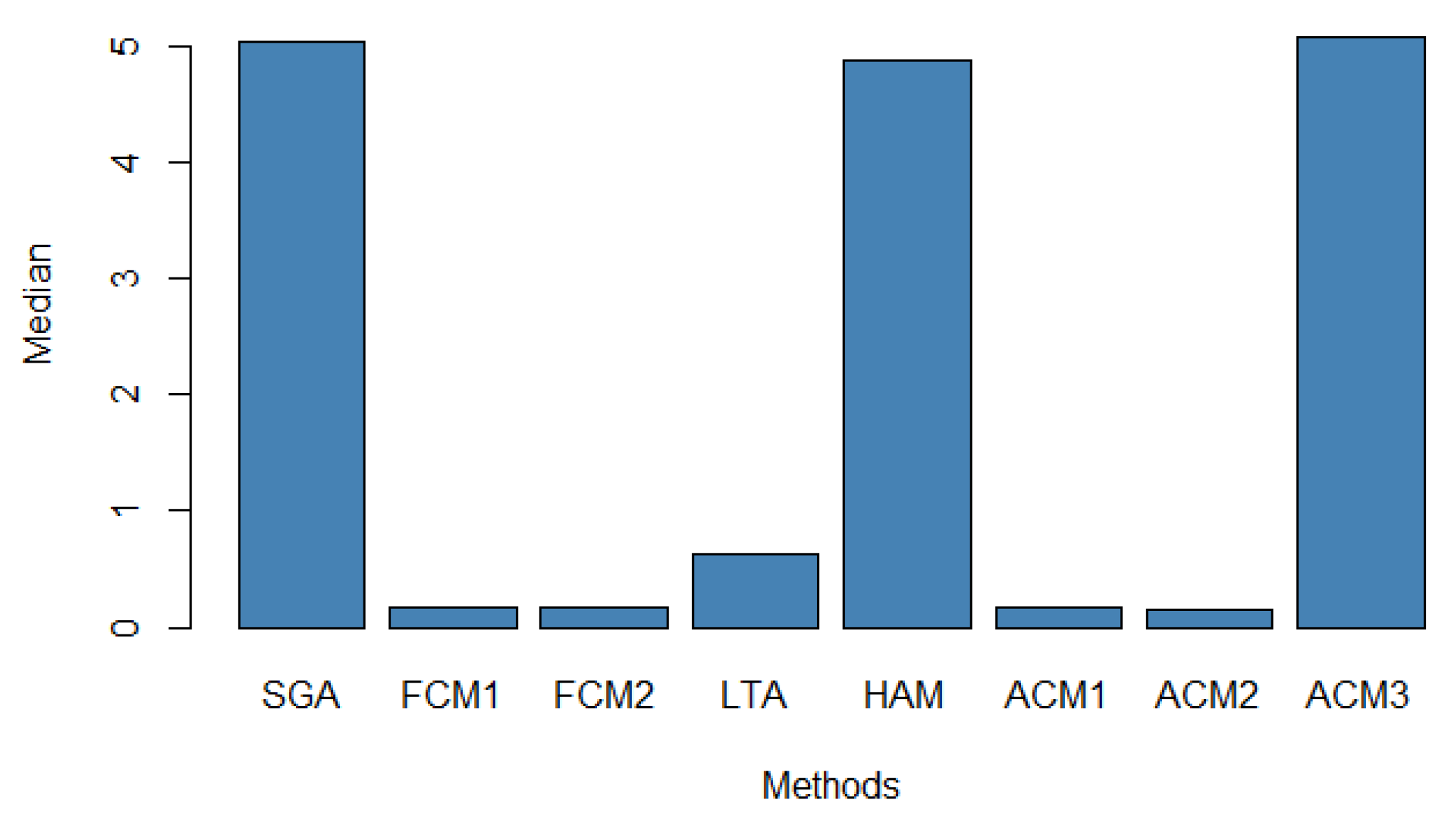
The median best fitness values are illustrated in Figure 9, where ACM2 achieved the lowest median. The ACM1, FCM1, and FCM2 were very close to ACM2. In contrast, SGA, HAM, and ACM3 showed much higher median values. The LTA was in between. In summary, the algorithms were ranked as ACM2 > FCM1 > FCM2 > ACM1 > LTA > HAM > ACM3 > SGA.

Overall, the ACM3 might offer the best possible outcome, but it severely lacks robustness and stability. Therefore, the ACM2 is the best candidate if the most rewarding but also balanced outcome is sought. The difference between their best is only 0.0001, and ACM2 is much more robust and stable, having the lowest median value among the methods. The FCM1 might have a better mean value than the ACM2, but given the stochastic nature of the runs, median values are more reliable.

5. Discussion

In this paper, the novel deterministic parameter methods, ACM1, ACM2, and ACM3, were proposed for the regulation of GA parameters. Their comparisons with an SGA, fixed-parameter GAs, and AGAs were made.

In the experiment for the smallest population size, the FCM2 achieved the lowest rank sum and stood out across both unimodal and multimodal functions, including non-separable ones. The methods ACM2, ACM1, and ACM3 followed the FCM2 closely, showing significant and stable results. When the population size increased to 50, the FCM2 remained where it was, achieving distinguished NCGO scores on most functions such as FN2, FN4, FN5, FN6, FN9, and FN10. The methods ACM1 and ACM3 followed the FCM2, with HAM and ACM2 also delivering good performances, especially in complex functions. The standard SGA and adaptive method, LTA, lagged behind with high variability and frequent failures on difficult problems. At the population size of 100, FCM2 ranked first again. The methods ACM1, HAM, and ACM2 performed very closely, with only slight reductions in NCGO for certain complex functions such as FN3 and FN8. The methods FCM1 and ACM3 also returned decent results, but with variability specific to the function in use. The LTA was inconsistent, achieving remarkable results in some cases but totally failing in others. The SGA performed the worst overall, unable to handle complex optimisation tasks consistently. The comparisons in this study confirmed that AGAs achieve a higher convergence rate than the standard GAs. According to the rank sum criterion and statistical tests, the SGA performs the worst.

For the next phases of the comparisons, larger and varying population sizes ($n=250,500,750$) and dimensions ($d=5,10,15$) were also utilised. The SGA was outperformed once again. For $d=5$, the methods ACM2, HAM, and FCM2 perform the best, taking the top of the ranks, with the lowest rank sum scores in the NCGO analysis. When the dimension was increased to $d=10$, ACM2 emerged as the best method, followed by FCM2 and HAM. This was a significant finding as it indicated that the ACM2 was a better choice for tackling higher-dimensional data. The question of how high the dimensions can reach brought out an important conclusion about the limits of the algorithms. For instance, consider the Rosenbrock function (FN8), despite the fact that the ACM1, ACM2, and HAM returned relatively better results, none of the methods were able to locate the global optimum, and all of them displayed the NCGO value of zero. Note that the FN8, by nature, is quite a challenging function, especially in high dimensions; thus, these results were merely a push of the limits of the algorithms. What is intriguing here is that, even in such a challenging scenario, the deterministic methods managed to converge closer to the optimum, with the ACM1, ACM2, HAM, and FCM2 achieving much better median values compared to SGA and LTA. For functions FN4 and FN7 at the dimension $d=15$, the ACM2 and HAM were the best, respectively. This shift in the performance leadership suggests the existence of problem-specific advantages among the top deterministic methods.

The comparative analysis of the GAs on the boost converter optimisation problem has validated the majority of the results obtained in the experiments with test functions. Once again, one of the FCMs and ACM2 have butted heads. However, ACM2 was the better choice with a lower median.

6. Conclusions

This study proposed three deterministic parameter control methods (ACM1–3) for Genetic Algorithms that offer a simple but computationally light alternative to adaptive schemes. The efficiency of the proposed methods was tested with rigorous benchmarking on multimodal and high-dimensional functions, along with a boost converter design optimisation. The tests included the comparisons of ACM1–3 with an SGA, two fixed-parameter GAs, an AGA, and another well-known deterministic method from the literature. Among the compared algorithms, ACM2 achieved the best balance in terms of convergence speed, stability, and scalability.

The most important implication of this study is that deterministic parameter control proves to be an effective and computationally efficient choice. As a result, despite the existence of an ever-increasing number of superior Evolutionary Algorithms, deterministic methods remain promising and relevant, especially for real-time applications or optimisation tasks where computational resources are limited.

For future work, we will investigate various new mechanisms to integrate into the AGAs. The proposed deterministic methods, ACM1, ACM2, and ACM3, will be tested to solve more complex engineering design problems and combinatorial optimisation problems. In this regard, real-world datasets are currently being sought for a subsequent engineering case study. In addition, the proposed methods can be extended to discrete or mixed-variable optimisation problems, which would be useful in real-world applications.

References

1. Holland, J.H. Adaptation in Natural and Artificial Systems; University of Michigan Press: Ann Arbor, MI, USA, 1975; pp. 5–97. [Google Scholar]
2. Katoch, S.; Chauhan, S.S.; Kumar, V. A Review on Genetic Algorithm: Past, Present, and Future. Multimed. Tools Appl. 2021, 80, 8091–8126. [Google Scholar] [CrossRef]
3. Kumar, M.; Hussain, M.; Upreti, N.; Gupta, D. Genetic Algorithm: Review and Application. Int. J. Inf. Technol. Knowl. Manag. 2010, 2, 451–454. [Google Scholar] [CrossRef]
4. Carr, J. An introduction to genetic algorithms. Sr. Proj. 2014, 1, 7. [Google Scholar]
5. Gen, M.; Lin, L. Genetic Algorithms and Their Applications. In Springer Handbook of Engineering Statistics; Springer: London, UK, 2023; pp. 635–674. [Google Scholar]
6. Goswami, R.D.; Chakraborty, S.; Misra, B. Variants of Genetic Algorithms and Their Applications. In Applied Genetic Algorithm and Its Variants: Case Studies and New Developments; Springer Nature: Singapore, 2023; pp. 1–20. [Google Scholar]
7. Waysi, D.; Ahmed, B.T.; Ibrahim, I.M. Optimization by Nature: A Review of Genetic Algorithm Techniques. Indones. J. Comput. Sci. 2025, 14, 268–284. [Google Scholar] [CrossRef]
8. Alhijawi, B.; Awajan, A. Genetic Algorithms: Theory, Genetic operators, Solutions, and Applications. Evol. Intell. 2024, 17, 1245–1256. [Google Scholar] [CrossRef]
9. Robles-Berumen, H.; Zafra, A.; Ventura, S. A Survey of Genetic Algorithms for Clustering: Taxonomy and Empirical Analysis. Swarm Evol. Comput. 2024, 91, 101720. [Google Scholar] [CrossRef]
10. Črepinšek, M.; Liu, S.H.; Mernik, M. Exploration and Exploitation in Evolutionary Algorithms: A Survey. ACM Comput. Surv. 2013, 45, 1–33. [Google Scholar] [CrossRef]
11. Patil, V.P.; Pawar, D.D. The Optimal Crossover or Mutation Rates in Genetic Algorithm: A review. Int. J. Appl. Eng. Technol. 2015, 5, 38–41. [Google Scholar]
12. Eiben, Á.E.; Hinterding, R.; Michalewicz, Z. Parameter control in evolutionary algorithms. IEEE Trans. Evol. Comput. 1999, 3, 124–141. [Google Scholar] [CrossRef]
13. McGinley, B.; Maher, J.; O’Riordan, C.; Morgan, F. Maintaining Healthy Population Diversity Using Adaptive Crossover, Mutation, and Selection. IEEE Trans. Evol. Comput. 2011, 15, 692–714. [Google Scholar] [CrossRef]
14. Basak, A. A Rank Based Adaptive Mutation in Genetic Algorithm. arXiv 2021, arXiv:2104.08842. [Google Scholar] [CrossRef]
15. Norat, R.; Wu, A.S.; Liu, X. Genetic Algorithms with Self-Adaptation for Predictive Classification of Medicare Standardized Payments for Physical Therapists. Expert Syst. Appl. 2023, 218, 119529. [Google Scholar] [CrossRef]
16. Liu, S.H.; Mernik, M.; Bryant, B.R. Entropy-Driven Parameter Control for Evolutionary Algorithms. Informatica 2007, 31, 41–50. [Google Scholar]
17. Smit, S.K.; Eiben, A.E. Using Entropy for Parameter Analysis of Evolutionary Algorithms. In Experimental Methods for the Analysis of Optimization Algorithms; Springer: Berlin/Heidelberg, Germany, 2010; pp. 287–310. [Google Scholar]
18. Fuertes, G.; Vargas, M.; Alfaro, M.; Soto-Garrido, R.; Sabattin, J.; Peralta, M.A. Chaotic Genetic Algorithm and the Effects of Entropy in Performance Optimization. Chaos 2019, 29, 013125. [Google Scholar] [CrossRef] [PubMed]
19. Lim, T.Y.; Tan, C.J.; Wong, W.P.; Lim, C.P. An Information Entropy-Based Evolutionary Computation for Multi-Factorial Optimization. Appl. Soft Comput. 2022, 114, 108071. [Google Scholar] [CrossRef]
20. Kaelo, P.; Ali, M.M. Some Variants of the Controlled Random Search Algorithm for Global Optimization. J. Optim. Theory Appl. 2006, 130, 253–264. [Google Scholar] [CrossRef]
21. Birattari, M.; Stützle, T.; Paquete, L.; Varrentrapp, K. A Racing Algorithm for Configuring Metaheuristics. In Proceedings of the Genetic and Evolutionary Computation Conference (GECCO 2002), New York, NY, USA, 9–13 July 2002; Volume 2. [Google Scholar]
22. Nannen, V.; Eiben, A.E. Efficient Relevance Estimation and Value Calibration of Evolutionary Algorithm Parameters. In Proceedings of the 2007 IEEE Congress on Evolutionary Computation (CEC 2007), Singapore, 25–28 September 2007; pp. 103–110. [Google Scholar]
23. Hutter, F.; Hoos, H.H.; Leyton-Brown, K.; Stützle, T. ParamILS: An Automatic Algorithm Configuration Framework. J. Artif. Intell. Res. 2009, 36, 267–306. [Google Scholar] [CrossRef]
24. Wang, L.; Shen, T. An Improved Adaptive Genetic Algorithm and its Application to Image Segmentation. In Proceedings of the SPIE 4550, Image Extraction, Segmentation, and Recognition, Wuhan, China, 21 September 2001. [Google Scholar]
25. Hassanat, A.; Almohammadi, K.; Alkafaween, E.; Abunawas, E.; Hammouri, A.; Prasath, V.B. Choosing mutation and crossover ratios for genetic algorithms: A review with a new dynamic approach. Information 2019, 10, 390. [Google Scholar] [CrossRef]
26. Srinivas, M.; Patnaik, L.M. Adaptive Probabilities of Crossover and Mutation in Genetic Algorithms. IEEE Trans. Syst. Man Cybern. 1994, 24, 656–667. [Google Scholar] [CrossRef]
27. Ren, Z.; San, Y. Improved Adaptive Genetic Algorithm and its Application Research in Parameter Identification. J. Syst. Simul. 2006, 18, 41–43. [Google Scholar]
28. Jiang, J.; Yin, S. A Self-adaptive Hybrid Genetic Algorithm for 3D Packing Problem. In Proceedings of the 2012 3rd Global Congress on Intelligent Systems, Wuhan, China, 6–8 November 2012; pp. 76–79. [Google Scholar]
29. Vandewater, L.; Brusic, V.; Wilson, W.; Macaulay, L.; Zhang, P. An Adaptive Genetic Algorithm for Selection of Blood-based Biomarkers for Prediction of Alzheimer’s Disease Progression. BMC Bioinform. 2015, 16, S1. [Google Scholar] [CrossRef]
30. Li, Y.B.; Sang, H.B.; Xiong, X.; Li, Y.R. An Improved Adaptive Genetic Algorithm for Two-dimensional Rectangular Packing Problem. Appl. Sci. 2021, 11, 413. [Google Scholar] [CrossRef]
31. Han, S.; Xiao, L. An Improved Adaptive Genetic Algorithm. SHS Web Conf. 2022, 140, 01044. [Google Scholar] [CrossRef]
32. Yu, W.J.; Shen, M.; Chen, W.N.; Zhan, Z.H.; Gong, Y.J.; Lin, Y.; Liu, O.; Zhang, J. Differential evolution with two-level parameter adaptation. IEEE Trans. Cybern. 2013, 44, 1080–1099. [Google Scholar] [CrossRef]
33. Wang, M.; Ma, Y.; Wang, P. Parameter and strategy adaptive differential evolution algorithm based on accompanying evolution. Inf. Sci. 2022, 607, 1136–1157. [Google Scholar] [CrossRef]
34. Cheng, L.; Zhou, J.X.; Hu, X.; Mohamed, A.W.; Liu, Y. Adaptive differential evolution with fitness-based crossover rate for global numerical optimization. Complex Intell. Syst. 2024, 10, 551–576. [Google Scholar] [CrossRef]
35. Takahama, T.; Sakai, S. Adaptive parameter control using search state estimation and extreme individuals for differential evolution. In Proceedings of the ISCIE International Symposium on Stochastic Systems Theory and its Applications (SSS), Tokyo, Japan, 17–18 November 2023; pp. 60–67. [Google Scholar]
36. Tanabe, R.; Fukunaga, A. Success-History Based Parameter Adaptation for Differential Evolution. In Proceedings of the 2013 IEEE Congress on Evolutionary Computation (CEC), Cancun, Mexico, 20–23 June 2013; pp. 71–78. [Google Scholar]
37. Tanabe, R.; Fukunaga, A.S. Improving the search performance of SHADE using linear population size reduction. In Proceedings of the 2014 IEEE Congress on Evolutionary Computation (CEC), Beijing, China, 6–11 July 2014; pp. 1658–1665. [Google Scholar]
38. Mohamed, A.W.; Hadi, A.A.; Fattouh, A.M.; Jambi, K.M. LSHADE with semi-parameter adaptation hybrid with CMA-ES for solving CEC 2017 benchmark problems. In Proceedings of the 2017 IEEE Congress on Evolutionary Computation (CEC), San Sebastian, Spain, 5–8 June 2017; pp. 145–152. [Google Scholar]
39. Fu, S.; Ma, C.; Li, K.; Xie, C.; Fan, Q.; Huang, H.; Xie, J.; Zhang, G.; Yu, M. Modified LSHADE-SPACMA with new mutation strategy and external archive mechanism for numerical optimization and point cloud registration. Artif. Intell. Rev. 2025, 58, 72. [Google Scholar] [CrossRef]
40. R Core Team. R: A Language and Environment for Statistical Computing; R Foundation for Statistical Computing: Vienna, Austria, 2025; Available online: https://www.R-project.org/ (accessed on 8 August 2025).
41. Cebeci, Z.; Tekeli, E.; Cebeci, C. adana: Adaptive Nature-Inspired Algorithms for Hybrid Genetic Optimization. R Package 2022, Ver 1.1.0. Available online: https://cran.r-project.org/web/packages/adana/index.html (accessed on 8 August 2025).
42. Surjanović, S.; Bingham, D. Virtual Library of Simulation Experiments: Test Functions and Datasets. Available online: http://www.sfu.ca/~ssurjano (accessed on 18 April 2025).
43. Bossek, J. smoof: Single- and Multi-Objective Optimization Test Functions. R J. 2017, 9, 103–113. [Google Scholar] [CrossRef]
44. Jamil, M.; Yang, X.S. A Literature Survey of Benchmark Functions for Global Optimisation Problems. Int. J. Math. Model. Numer. Optim. 2013, 4, 150–194. [Google Scholar] [CrossRef]
45. Michalewicz, Z. Genetic Algorithms, Numerical Optimization, and Constraints. In Proceedings of the 6th International Conference on Genetic Algorithms, Pittsburgh, PA, USA, 15–19 July 1995; Morgan Kaufmann: San Mateo, CA, USA, 1995; pp. 151–158. [Google Scholar]
46. Michalewicz, Z.; Logan, T.; Swaminathan, S. Evolutionary Operators for Continuous Convex Parameter Spaces. In Proceedings of the 3rd Annual Conference on Evolutionary Programming, San Diego, CA, USA, 24–26 February 1994; World Scientific Publishing: Hackensack, NJ, USA, 1994; pp. 84–97. [Google Scholar]
47. Hogg, R.V.; Tanis, E.A.; Zimmerman, D.L. Probability and Statistical Inference, 7th ed.; Macmillan: New York, NY, USA, 1977. [Google Scholar]
48. Kar, S.S.; Ramalingam, A. Is 30 the Magic Number? Issues in Sample Size Estimation. Natl. J. Community Med. 2013, 4, 175–179. [Google Scholar]
49. Hays, W.L. Statistics, 5th ed.; Holt, Rinehart and Winston: New York, NY, USA, 1994. [Google Scholar]
50. Erickson, R.W.; Maksimović, D. Fundamentals of Power Electronics, 3rd ed.; Springer: Cham, Switzerland, 2020. [Google Scholar]
51. Shilane, D.; Martikainen, J.; Dudoit, S.; Ovaska, S.J. A General Framework for Statistical Performance Comparison of Evolutionary Computation Algorithms. Inf. Sci. 2008, 178, 2870–2879. [Google Scholar] [CrossRef]
52. Picheny, V.; Wagner, T.; Ginsbourger, D. A Benchmark of Kriging-based Infill Criteria for Noisy Optimization. Struct. Multidiscip. Optim. 2013, 48, 607–626. [Google Scholar] [CrossRef]
Figure 1. Boost converter circuit diagram.
Applsci 15 11093 g001
Figure 2. Changes in crossover and mutation rates across the generations in deterministic methods (a) HAM; (b) ACM1; (c) ACM2; and (d) ACM3.
Applsci 15 11093 g002
Figure 3. Median comparison of GAs across benchmark functions (n = 20).
Applsci 15 11093 g003
Figure 4. Comparison of GAs across benchmark functions (n = 50).
Applsci 15 11093 g004
Figure 5. Comparison of GAs across benchmark functions (n = 100).
Applsci 15 11093 g005
Figure 6. Comparison of GAs across benchmark functions (d = 5 and n = 250, gmax = 100).
Applsci 15 11093 g006
Figure 7. Comparison of GAs across benchmark functions (d = 10 and n = 500).
Applsci 15 11093 g007
Figure 8. Comparison of GAs across benchmark functions (d = 15 and n = 750).
Applsci 15 11093 g008
Figure 9. Median values of the best fitness values across generations.
Applsci 15 11093 g009