Article

Deterministic Modeling of Muller’s Ratchet Effect in Populations Evolving in an Environment of Finite Capacity

1
Department of Computer Graphics, Vision and Digital Systems, Silesian University of Technology, Akademicka 16, 44-100 Gliwice, Poland
2
Department of Applied Informatics, Silesian University of Technology, Akademicka 16, 44-100 Gliwice, Poland
*
Author to whom correspondence should be addressed.
Appl. Sci. 2025, 15(20), 11090; https://doi.org/10.3390/app152011090
Submission received: 27 August 2025 / Revised: 10 October 2025 / Accepted: 14 October 2025 / Published: 16 October 2025
(This article belongs to the Special Issue Research on Computational Biology and Bioinformatics)

Abstract

We study how small harmful mutations spread in populations that reproduce asexually. This process is known as Muller’s ratchet—it means that even though these mutations are damaging, they can still build up over generations. To explore this, we use a mathematical model that describes how such mutations move through a population living in an environment with limited resources. We model Muller’s ratchet deterministically using differential equations, incorporating modifications that account for extinction risk of small mutation classes. We analyze two modifications: a published cutoff modification and a more flexible exponential modification. We show that the exponential modification better matches stochastic simulations over specific parameter ranges.

1. Introduction

In asexual populations with mildly deleterious mutations, these mutations accumulate despite their genetic disadvantage. Because recombination is absent, accumulated deleterious mutations are irreversible and can ultimately cause population extinction. The scenario of the advancement of a deleterious mutation wave/front in a population, dependent on the population size, is called Muller’s ratchet [1,2], or the mutational meltdown effect [3,4]. The accumulation of mildly deleterious mutations and their effects was experimentally studied/observed in several models/scenarios of the asexual evolution of populations of species, organisms, and cells. Some examples include the Y chromosome [5], mitochondria [6], aging [7,8], viral infections [9,10], and cancers [11,12,13].
Numerous studies reproduce Muller’s ratchet in stochastic simulations and use mathematical models to examine the propagation and effects of weakly deleterious mutations.
In classical deterministic models of the evolution of an asexually reproducing population of constant size (in Wright–Fisher or Moran models) affected by mildly deleterious mutations, individuals (species, organisms, cells) with a higher mutational load are under stronger negative selection, leading to a Poisson-like stationary mutation front/wave [2]. In stochastic simulations corresponding to these models, the mutation front is not stationary but undergoes a slow advancement/propagation. The advancement of the mutation wave results from random genetic drift, which threatens the survival of the least-loaded class (individuals carrying the fewest mutations). Several studies have developed quantitative, analytical, or semi-analytic methods for estimating the propagation speed of a mutation wave [14,15,16,17,18]. Some approaches involve modeling propagation of deleterious mutations that lead to shrinking of the population. Research initiated by [3,4] aimed to estimate both the speed of propagation of the mutation wave and the dynamics of the shrinkage of the population size in asexual evolutionary models with mildly deleterious mutations. These investigations were further developed to estimate the time to extinction in populations with deleterious mutations with high mutation rates [19]. Some recent publications have analyzed Muller’s ratchet effect in near-critical regimes [20], the strength of genetic drift in large populations and implications of the ratchet effect [21], and Muller’s ratchet in a structured coalescent framework [22]. An interesting approach is to introduce modification/modifications to deterministic model equations, resulting in better consistency between deterministic and stochastic model solutions. It was observed/discovered that introducing the cutoff function/condition to the component representing the rate of the birth process allows for better consistency between deterministic modeling of evolution and stochastic simulations. The cutoff condition proposed in [23] and further mentioned in [24,25,26] stops events of cell (individual) births in cases where the number of cells is less than one and (since only deaths become possible) mimics the effects of the occurrence of extinction of the least-loaded class. Introducing the cutoff condition allows one to reflect Muller’s ratchet mechanism in deterministic modeling.
In this paper, we study a model of population evolution that undergoes changes in size in response to weakly deleterious mutations within an environment characterized by finite capacity. The scenario analyzed, with random events of deaths, births, and weakly deleterious mutations, and is related to that originally published in [12]. The model in [12], more complicated compared to ours, included two types of mutation, deleterious and advantageous. Depending on the values of the parameters, the cellular population modeled in [12] can experience growth or decline. Here, the scenario under study is restricted to the case of population decline caused by deleterious mutations. We elaborate both stochastic and deterministic models, and our analyses aim at achieving agreement between deterministic and stochastic modeling. In our deterministic model we implement the cutoff condition, and we also propose an improvement/modification of the cutoff approach by introducing an exponential function for determining the reduction in the rate of the birth process caused by genetic drift. We compare all models of evolution studied.
Consistent with prior studies, concerning scenarios of constant population size evolution, the deterministic model of evolution with mildly deleterious mutations, in an environment of finite capacity, again leads to a stationary mutation front, while in stochastic simulations, the mutation wave moves forward with a speed dependent on the population size. Modifications to the cutoff and exponential in deterministic balance equations, reflecting the risk of extinction of mutation classes, allow one to see better consistency between deterministic and stochastic modeling. A comparison of the ability of the cutoff and exponential functions to reflect the Muller ratchet effect indicates better performance in the latter.

2. Methods

Key assumptions of our model are as follows:
  • Evolution is asexual, with events of births (replications), deaths and mutations.
  • The population comprises individuals, species, organisms or cells of different reproductive fitness.
  • The population is under pressure from an environment of finite capacity, where the size of the population modifies the rate of the death process.
  • Random, weakly deleterious mutations take place during birth processes. They modify reproductive fitness of individuals.
Events in the analyzed scenario of evolution are shown graphically in Figure 1. Deaths and births of individuals in the population are inhomogeneous. Poisson processes have rates depending on the population size and the numbers of mutations carried by individuals. The occurrence of random mutations can accompany events of births.

2.1. Evolution of Population with Mutation and Selection in an Environment of Finite Capacity

In the following, we describe, in quantitative terms, processes of death, birth, and mutation. The rate of the death process, denoted by μ D ( N ) , depends on the population size N and the parameter of environmental capacity N C , and is calculated using the relation
μ D ( N ) = N N C .
The group of individuals, each carrying the same number k of mutations, is named class k or type k. Births in class k follow a Poisson process with a rate of μ B ( k , s ) defined by
μ B ( k , s ) = 1 ( 1 + s ) k e k s .
Here s is the weak negative selection coefficient; the approximation holds for small s. The rate of the birth process (2) can be used to scale the time lapse. We assume that the unit of time is the waiting time for the birth of the individual in a case where k = 0 . In other words, the unit of time is the expectation, in the exponential distribution, of the waiting time for the first event of birth resulting from the rate (2) with k = 0 , μ B ( 0 , s ) = 1 .
Mutations occur during divisions, with probability p s , which leads to the rate given by
p s μ B
where μ B is the rate of the birth process given by (2).
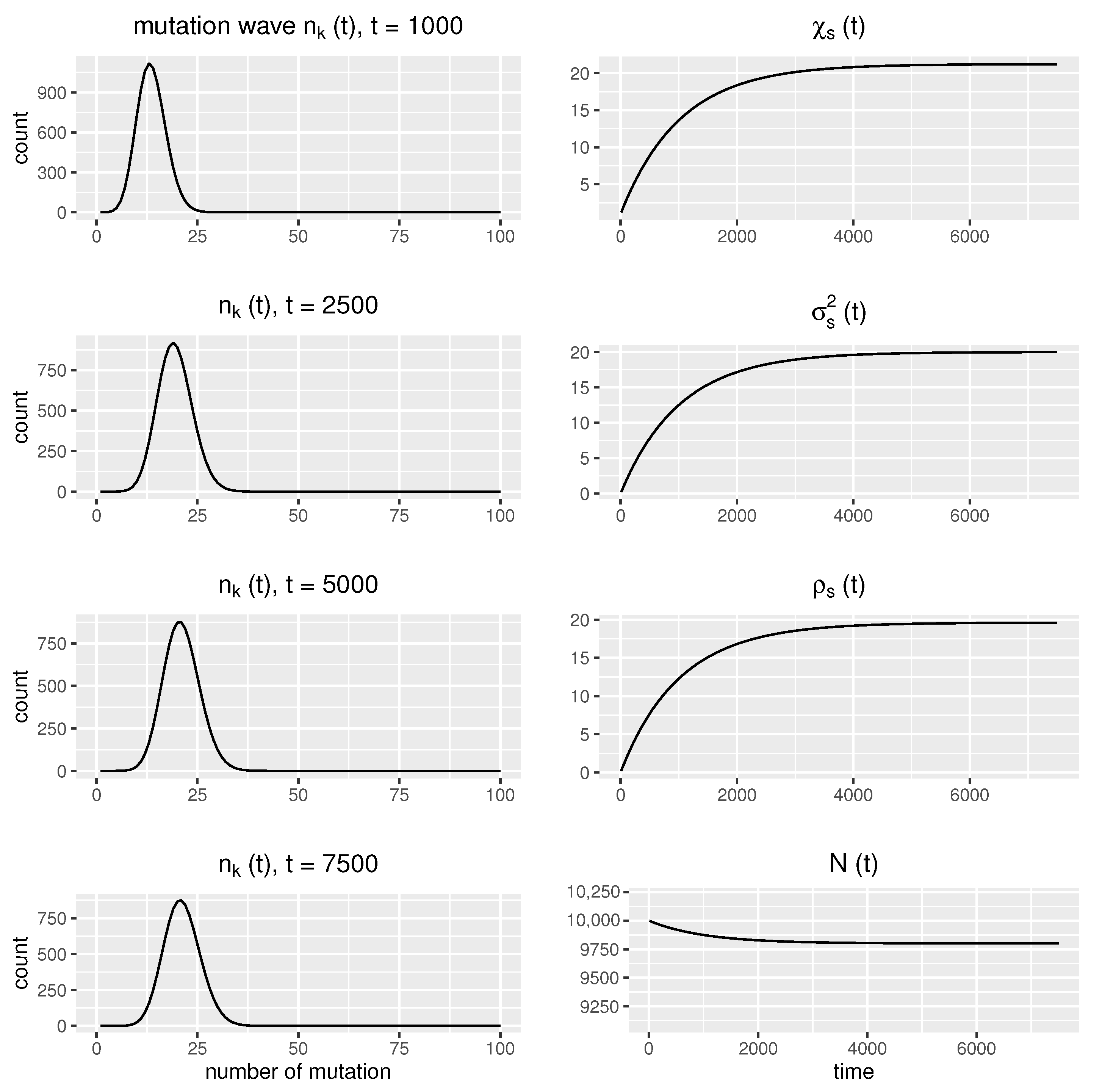
Following the above assumptions, in this paper, as shown in Figure 2, Figure 3 and Figure 6, we introduce a system for representing results of deterministic modeling and stochastic simulations with two columns of plots. In this system the positions of mutation waves are drawn in the left column (at four time points chosen from the computation/simulation horizon), while the right column presents time plots of parameters of mutation propagation in the population, mean number of deleterious mutations (upper plot), variance in the number of deleterious mutations (second plot from the top), third central moment of the number of mutations (third plot from the top), and population size (lower plot).

2.2. Deterministic Model of Propagation of Weakly Deleterious Mutations in Population Evolution

The construction of the deterministic model of the propagation of weakly deleterious mutations for the evolution of the population in an environment with a capacity of N C is based on formulating differential equations for the expected rates of changes in the number of individuals in the population and the expected rates of changes in the number of mutations harbored by individuals.

2.3. Deterministic Balance Equations

Based on relations (1)–(3) we can formulate the system of differential equations of the balance of numbers of individuals and mutations following from divisions/births, deaths and mutations. They assume the following form:
d d t n k = p s μ B ( k 1 , s ) n k 1 + ( 1 p s ) μ B ( k , s ) n k μ D ( N ) n k ,
The right-hand side has three components. The first component is the rate of increase in the number of individuals of type k due to individuals of type k 1 acquiring mutations during their births/replications; the second component gives the rate of increase due to replications of individuals of type k; and finally, the third is the rate of decrease due to deaths. The range of indices k is k = 1 , 2 .

2.4. Evolution of the Population Size

Denote as N the total number of individuals in the population, equal to the sum of the numbers of individuals in all classes N = k n k . Denote the mean and variance in the number of weakly deleterious mutations at time t as χ s ( t ) and σ s ( t ) , respectively.
χ s ( t ) = χ s = k k ν k ,
σ s 2 ( t ) = σ s 2 = k ( k χ s ) 2 ν k .
In (5) and (6), ν k ( t ) = ν k are frequencies of individuals of type k.
ν k ( t ) = ν k = n k ( t ) N ( t ) .
Based on the assumption of a mild/weak effect of mutations, we linearize the birth rate function μ B ( k , s ) in Equation (2) around the mean value (5). The linearized relation (2), μ B ( k , s ) e χ s s s e χ s s ( k χ s ) , formulated for the values k and k 1 gives rise to the formulas
μ B ( k , s ) μ B ( χ s , s ) 1 s ( k χ s ) ,
μ B ( k 1 , s ) μ B ( χ s , s ) 1 s ( k 1 χ s ) ,
which are used in the subsequent derivations.
Summing both sides of Equation (4) over the range of values of k and using the linear approximations (8) and (1), we get
d d t N = μ B ( χ s , s ) N N C N .
The above differential equation describes the dynamics of the size of the population N ( t ) . Its solution exhibits fast and slow timescales [27]. In the fast timescale, we have μ B ( χ s , s ) c o n s t , so, starting from any initial condition, the population size N ( t ) tends to the fast time limit N = N C μ B ( χ s , s ) . In the slow timescale, we use the approximation d d t N N 0 , which gives the slow-timescale dynamics of the population size.
N ( t ) = N C μ B ( χ s ( t ) , s ) .
The evolution of population size in the slow timescale (11) is determined by the time changes for the mean numbers of mutations in cells χ s ( t ) . Weakly deleterious mutations that occur in evolution are slowly changing/increasing the value of χ s ( t ) . The accumulation of weakly deleterious mutations results in a slow decrease in population size. The mathematical model of the change in χ s ( t ) is derived in Section 2.5 and Section 2.6.

2.5. Equations for Evolution of Frequencies of Classes

In this subsection, we derive equations that describe the dynamics of frequencies of individuals’ types/classes. These equations are necessary to derive relations for the dynamics of traveling mutation waves in Section 2.6.
In order to derive equations for frequencies ν k ( t ) given by (7) we first differentiate both sides of (7) to obtain
d d t ν k = 1 N 2 d N d t n k + 1 N d n k d t .
Now, substituting (10) and (4) in the above equation and again using (9), we have
d d t ν k = μ B ( χ s , s ) p s ( 1 s ( k 1 χ s ) ) ν k 1 p s ( 1 s ( k χ s ) ) ν k s ( k χ s ) ν k .

2.6. Traveling Waves of Mutations

The result of the previous subsection allows us to derive equations for the dynamics of changes in the mean number of mutations in cells/individuals χ s ( t ) , which describe the positions of mutation waves. Multiply both sides of Equation (13) by k and add up the range of indices k. This leads to
k k ( d d t ν k ) = d d t ( χ s ) = μ B ( χ s , s ) ( p s s σ s 2 ) .
Equation (14) relates the speed of the advancement in the weakly deleterious mutation wave to the values of the model parameters, the mutation probability p s and the selection coefficient s, and to the variance σ s 2 (width of the mutation wave). The mean number of mutations χ s is the position of the mutation wave in the population, while the variance σ s 2 defines the width of the wave. Equation (14) is analogous to many similar relations derived in the literature [3,4,26,28]. This relation is very useful for modeling propagation of the mutation wave. Using (14) to predict the motion of the mutation wave requires computing/estimating σ s 2 ( t ) .

2.7. Stationary Mutation Front

In this subsection, we show a methodology for solving the dynamics of the mutation wave motion. We show that the deterministic model (4) leads to a stationary mutation front analogous to the stationary Poisson-like distribution in the Haigh model [2]. By multiplying both sides of Equation (13) by ( k χ s ) 2 and again summing up over the range of indices k, we obtain the following differential equation for the time evolution of variance σ s 2 ( t ) .
d d t ( σ s 2 ) = μ B ( χ s , s ) [ p s ( 1 2 s σ s 2 ) s ρ s ]
where ρ s is the third central moment.
ρ s ( t ) = ρ s = k ( k χ s ) 3 ν k .
Analogously to Equation (14), in the above equation, the higher moment ( ρ s ) appears in the differential equations for a lower moment ( σ s 2 ). This problem can be solved by assuming that the shape of the mutation wave remains stationary over time. Equivalently, assume that the following approximation holds:
d d t n k ( n k n k 1 ) d d t ( χ s ) = ( n k n k 1 ) μ B ( χ s , s ) ( p s s σ s 2 ) .
The second equation above follows from using (14). Substituting d d t n k from (17) in the differential Equation (4) leads (after simple transformations) to a recurrent equation for the shape of the mutation wave:
[ σ s 2 + ( 1 p s ) ( k χ s ) ] n k = [ σ s 2 p s ( k 1 χ s ) ] n k 1 .
This recurrence yields a relationship between σ s 2 and ρ s . By multiplying both sides of (18) by ( k χ s ) 2 and adding up the range of values of k, we obtain
ρ s = σ s 2 ( 1 2 p s ) ,
which transforms Equation (15) into
d d t ( σ s 2 ) = μ B ( χ s , s ) ( p s s σ s 2 ) .
The above differential equation has a stable equilibrium.
σ s 2 = p s s .
Substituting σ s 2 from (21) into Equation (14) for the evolution of χ s leads to a stationary front of mutations:
d d t ( χ s ) = 0 .
From (21), (22) one can see that, in the deterministic model (4), for an arbitrary small positive value of the selection coefficient s, the process of the advancement of the mutation front is counterbalanced by the deleterious effect of mutations, leading to the stationary distribution of mutations. The stationary mutation front for the deterministic model (4) is analogous to the stationary Poisson-like distribution for the Wright–Fisher model with a constant-size population [2].
In order to illustrate the derived relations, in Figure 2 we show the scenario of mutation propagation, with the results obtained by the numerical solution to differential Equation (4) assuming the following parameters: s = 0.001 , p s = 0.02 , N C = 10,000. The initial conditions for the computations were n 0 ( 0 ) = N C , n k ( 0 ) = 0 , k = 1 , 2 , . The left part of Figure 2 shows propagation of the computed mutation wave represented by the positions of the wave at time points t = 1000 , t = 2500 , t = 5000 and t = 7500 . The propagation of the mutation wave is also illustrated in the right panel of Figure 2 by time plots of χ s ( t ) (mean numbers of mutations, upper plot), σ s 2 ( t ) (variance in mutation numbers), ρ s ( t ) (third central moment of mutation numbers) and N ( t ) (population size, lower plot). The propagation scenario in Figure 2 is consistent with the analytical results (19)–(22) derived above.
The mutation wave eventually reaches a stationary state, with values of variance and third central moment ( σ s 2 = 20 = p s s and ρ s = 19.6 σ s 2 ( 1 2 p s ) ) close to those predicted by Equations (19) and (21).
The conclusion arising from (14) and (20), confirmed by the numerical solution to (4), is that when the initial values of χ s and σ s 2 are zero ( χ s ( 0 ) = 0 , σ s 2 ( 0 ) = 0 ), the mean number of mutations in the individual, χ s ( t ) , saturates at approximately
lim t χ s ( t ) p s s .
Figure 2. The left panels present mutation wave profiles at four time points (from top to bottom: t = 1000 , t = 2500 , t = 5000 and t = 7500 ). The right panels display temporal dynamics of the mean number of mutations, χ s ( t ) (upper plot); the variance of mutation numbers, σ s 2 ( t ) ; the third central moment of mutation numbers, ρ s ( t ) ; and the population size N ( t ) , defined as the total number of individuals in the population (lower plot).
Applsci 15 11090 g002

2.8. Deterministic Modeling Versus Stochastic Simulations

The evolution of the population with the events shown in Figure 1, further quantitatively characterized in expressions (1)–(3), can be simulated stochastically by using the Gillespie algorithm [29,30,31]. In the Gillespie simulation algorithm, random times of events of deaths, divisions, and mutations are generated on the basis of intensities in expressions (1)–(3). In our implementation, the state of the process is N—a dimensional vector where N is the population size. Each element of the state vector corresponds to an individual, and its value specifies the number k of mutations acquired by the individual. Initially, all values of k are equal to 0, since the initial mutation number is zero in relation to the environmental capacity, N = N C . We use tau-leap version of the Gillespie algorithm [31]. In one simulation cycle, we record events of deaths, births, and mutations, whose time points, randomly drawn from appropriately defined distributions, are less than tau. In the calculations used, the tau values were in the range of 0.005 τ 0.05 .
Using the elaborated algorithm, we have stochastically simulated the evolution of the population with the same parameters as shown in Figure 2, starting from the same initial conditions. A comparison of the results of the stochastic simulations and deterministic computations is shown in Figure 3. The black lines represent the deterministic solutions computed using the numerical integration of (4), already drawn in Figure 2, while the red plots show the results of the stochastic simulations using the Gillespie algorithm. The comparison shows significant differences. At first, both waves are in similar positions. However, later the deterministic wave freezes at a certain point, while the wave obtained in stochastic simulations constantly moves towards the right. As a result, in the deterministic case, the population size stabilizes at a certain level, while in the stochastic simulations, it decreases. The progression of the mutation wave in the stochastic simulations and the related decrease in population size in Figure 3 are effects of Muller’s ratchet.
Figure 3. Comparison of stochastic simulations and deterministic modeling for the evolution of a population with weakly deleterious mutations. The parameters and layout are the same as in Figure 2. Black solid lines correspond to deterministic results obtained by numerical integration of >Equation (4), while red lines represent stochastic simulations using Gillespie algorithm.
Applsci 15 11090 g003

3. Results

As derived in Section 2.7 and illustrated in Figure 2 and Figure 3, the deterministic model (4) predicts the occurrence of the stationary mutation front, whereas in stochastic simulations, advancement of the mutation wave is observed. The mutation wave obtained in the stochastic simulations, seen in Figure 3 (in red), showing random variations, is narrower than the corresponding deterministic one (in black). This is seen when comparing the red (stochastic) and black (deterministic) time plots of the variances in the mutation wave in the right panel of Figure 3. The red plot corresponding to the stochastic simulation has significantly lower values than the black plot that represents the deterministic solution. This is consistent with Equation (14), which describes the advancement of the mutation wave, where lower values of the variance in mutation numbers σ s 2 ( t ) result in a faster mutation wave speed.

3.1. Modified Deterministic Models

Here we address the problem stated in Section 1 of introducing modification/ modifications to the balance Equation (14), aiming at obtaining better consistency between the solutions to systems of deterministic balance equations and the results of stochastic simulations. In the following, we describe two such modifications of the deterministic balance equations, which we name cutoff and exponential modifications.

3.2. Cutoff Modification

The first approach to modification, named the cutoff modification/condition, uses the factor function F c u t o f f ( n k ) given below.
F c u t o f f ( n k ) = 0 if n k < 1 1 if n k 1
The function of the above factor is related to the hypothesis that cell division in the class of individuals that harbor k mutations can only occur if there is at least one cell in the class; otherwise, the value of the rate of birth for that class is set to zero. The issue of the influence of fractional values of n k on the dynamics of the mutation front does not arise in the stochastic model, which deals only with integer values of n k , but it does arise in the deterministic model, where fractional values occur. Applying the above factor F c u t o f f ( n k ) to the balances of cells and mutations results in the following modified form of deterministic balance equations.
d d t n k = p s μ B ( k 1 , s ) F cutoff ( n k 1 ) n k 1 + ( 1 p s ) μ B ( k , s ) F cutoff ( n k ) n k μ D ( N ) n k .
The right-hand sides of Equation (25), due to the factor function F c u t o f f ( n k ) , become discontinuous, so their solutions should be interpreted in a suitable way [32].

3.3. Exponential Modification

The second modification, called exponential modification, is described by a factor function F e x p ( n k ) :
F e x p ( n k ) = ( 1 e α n k )
where α is a function parameter. The factor given by the above equation is a function that gradually reduces the probability of birth in classes with a low number of individuals and does not affect classes with a larger number of individuals. The exponential factor for reducing birth rate may be closer to reality due to the fact that the least-loaded class, as well as other classes with a low number of individuals, are at risk of extinction.
Applying the above factor (26) to birth rates results in the following form of balance equations:
d d t n k = p s μ B ( k 1 , s ) F exp ( n k 1 ) n k 1 + ( 1 p s ) μ B ( k , s ) F exp ( n k ) n k μ D ( N ) n k .

3.4. Characterization and Comparison of Two Modifications

Introducing a modification to the deterministic balance equations, cutoff (25) or exponential (27), changes the dynamics of the propagation of weakly deleterious mutations in the population. In this subsection, we analyze the effects of these modifications in more detail.

3.4.1. Stationary Mutation Fronts Versus Advancing Mutation Waves

Compared to the deterministic balance model (4), models with cutoff modification (25) and with exponential modification (27) show more complex dynamics. In particular, both modified models can show either a stationary mutation front or an advancing mutation wave, depending on the values of the parameters. For a given set of parameters, N C , s, p s and α , the existence of a stationary mutation front can be interpreted as the existence of stable equilibrium of the system of differential equations either (25) for the model with cutoff modification or (27) for the model with exponential modification. A standard method for the analysis of (local) stability is linearization of the system of differential equations in the vicinity of equilibrium and application of stability conditions for linear multivariable systems, e.g., [33].
For the model with cutoff modification (25), the linearization approach is impossible due to the discontinuity of the right-hand sides. However, the simplicity of the cutoff modification allows one to formulate the following approximate condition for stationarity of the mutation front. Accept the following assumptions:
  • The least-loaded class is n 0 .
  • The stationarity condition is
    n 0 > 1 .
  • The shape of the stationary mutation wave can be approximated by Poisson distribution with χ s = σ s 2 = p s s (see Equations (21) and (23)).
Then using n 0 N e p s s N C e p s s , one can write inequality (28) as
N C e p s s > 1 .
The simplifications used to derive (29) are twofold. First, the shape of the stationary mutation wave is not exactly Poisson. Second, the condition (28) ensures that the cutoff factor function does not influence the dynamics of the size of the least-loaded class, but the possible influence of the cutoff factor function on the change in the size of the most-loaded class is ignored. Despite simplifications, the condition (29) works reasonably well when verified by numerical solutions to the system of differential Equation (25).
The condition of the form (29) is well known in the literature about deleterious mutations that propagate in a population of constant size [34], where it is used for distinguishing between shapes of the traveling mutation wave (Poisson versus negative binomial).
The model with exponential modification (27) allows for the linearization approach. The local stability condition is obtained by computing the eigenvalues of the state matrix of the linearized model, and the stationarity of the mutation front can be predicted with better accuracy. However, in contrast to the cutoff model, here there is no simple analytical formula. The existence of a stationary front versus an advancing mutation wave is determined by a numerical (computational) procedure.
As examples of using the approaches described above, assume the following values for the coefficient of selection and probability of mutation: s = 0.006 and p s = 0.05 . In the model with cut-off modification, the application of condition (29) with N C = 1000 , N C = 5000 and N C = 10,000 leads, respectively, to the following values of the left-hand side of (29): N C e p s s = 0.2404 , N C e p s s = 1.2018 and N C e p s s = 2.4037 . Verification by numerical integration of (25) reveals that the values of N C = 1000 and N C = 10,000 imply an advancing wave and a stationary front, respectively. However, for N C = 5000 one observes an advancing wave as a numerical solution to (25), contrary to the prediction of (29).
In the model with exponential modification, assume the same values of the coefficient of selection and probability of mutation as before ( s = 0.006 and p s = 0.05 ). Take α = 0.12 . One can verify that the stationary mutation front will be seen in the case of N C > 490,000, while the advancing mutation wave will correspond to N C < 490,000.
Summing up the above example, in the model with exponential modification, we can predict the stationarity of the mutation front versus the advancing mutation wave by using a numerical procedure involving linearization of model equations, without the need for numerical integration of model Equation (27). For the case of cutoff modification, we can predict the stationarity of the mutation front versus the advancing mutation approximately, using condition (28), without the need for numerical integration of differential Equation (25). Exact prediction is possible, but requires numerical integration of differential Equation (25).

3.4.2. Numerical Computations for Comparative Analysis of the Positions of Mutation Waves at Various Time Points

In order to more thoroughly assess the impact of the two modifications of the deterministic balance equations on improving the fit between deterministic and stochastic modeling, the results of a series of stochastic Gillespie simulations were compared with numerical solutions to models (25) and (27). These computational experiments were performed for the parameter s in the range of < 0.0001 ; 0.005 > and the parameter p s in the range of < 0.001 ; 0.05 > . For all calculations, the values N C = 10,000 and α = 0.12 (in model (27)) were used. In total, 121 stochastic simulations were performed for various combinations of parameters s and p s . The simulations spanned 7500 generations, with data collected every 50 generations.
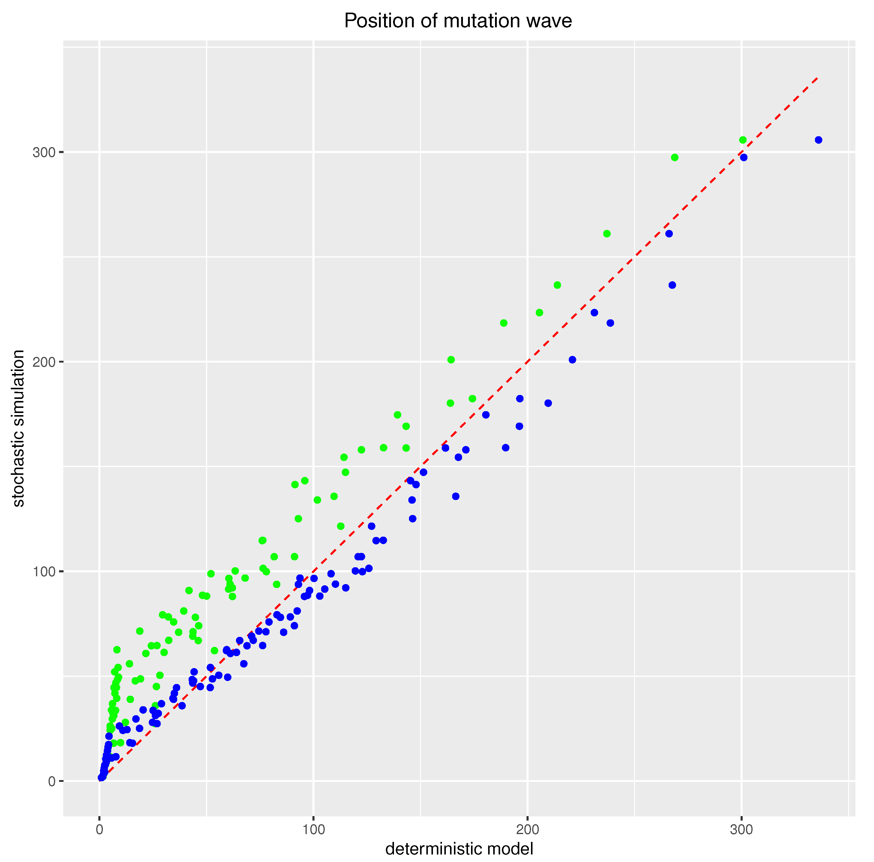
The results of the computational experiments described above are presented in Figure 4 as two color scatter plots, where green corresponds to the comparison between the dynamics of model (25) (cutoff modification) and the stochastic simulations, and blue is used for comparisons between the dynamics of model (27) (exponential modification) and the stochastic simulations. Each circle, green and blue, represents one comparison of the position of the mutation wave obtained in the deterministic computations (with either cutoff or exponential modification) to the corresponding position of the mutation wave (with the same parameters) obtained in the stochastic simulations.
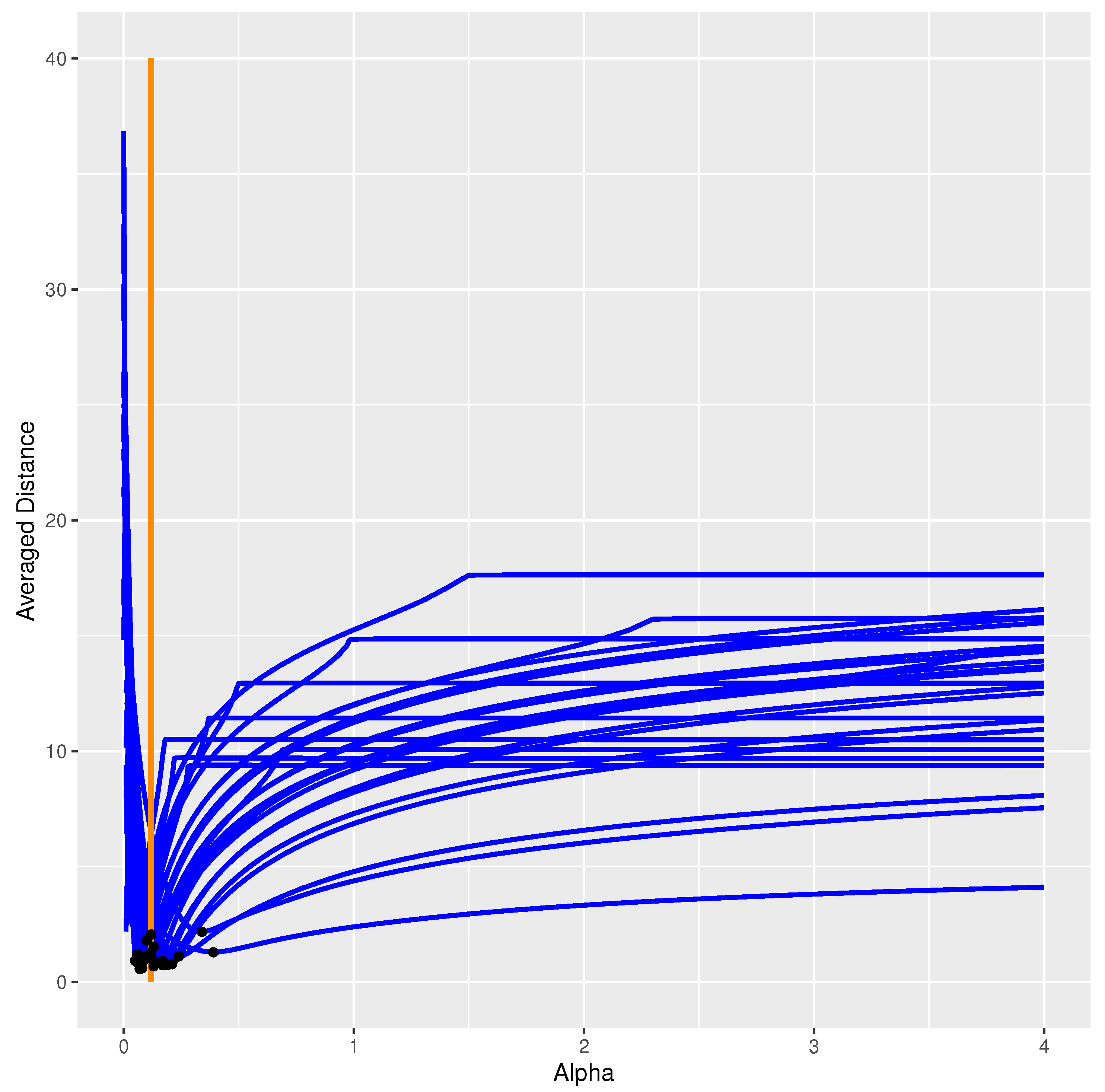
The choice of the parameter α was based on minimizing the average absolute distance, denoted by D, between the positions of the mutation waves obtained in the deterministic model (with exponential modification with parameter α ) and stochastic simulations. The value of D is therefore given by the following formula:
D = 1 N U M e x p e r i m e n t s | χ s d e t e r m i n i s t i c ( t k ) χ s s t o c h a s t i c ( t k ) | .
In the above equation, by “experiments”, we mean the grid of values of selection coefficients s < 0.0001 ; 0.005 > (25 values) and time points t k < 50 ; 7500 > (150 values), which results in N U M = 150 × 25 = 3750 . The positions of the mutation wave in the deterministic model and stochastic simulations (for selection coefficient s, at time point t k ) are denoted, respectively, by χ s d e t e r m i n i s t i c ( t k ) and χ s s t o c h a s t i c ( t k ) .
Based on the above definition of average distance D, the minimal distance value was identified and the corresponding value of α was recorded as α = 0.12 . We also performed a sensitivity analysis to investigate how variations in the parameter α affect the behavior of the model. Specifically, an experiment was designed to test s in the range of < 0.0001 ; 0.005 > , and α in the range of 0 to 4. For each parameter value s, an average distance measure was calculated across time points t k < 50 ; 7500 > . The results are shown graphically in Figure 5.
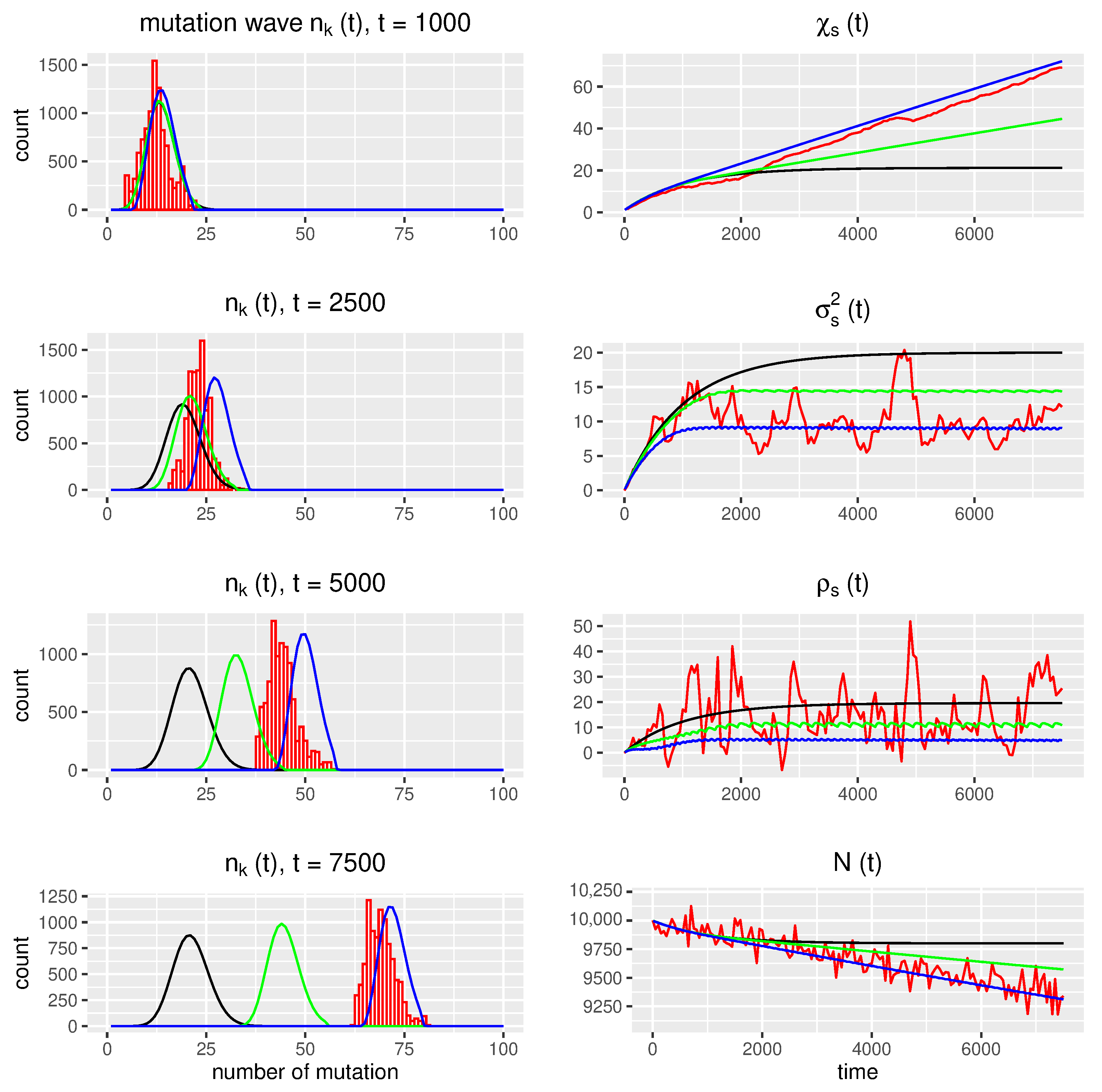
In Figure 6, we additionally present one comparison of the numerical solutions to the deterministic model without modification (black) and the deterministic model with cutoff modification (green) or exponential modification (blue), and the results of the stochastic simulations (red), for the same evolutionary scenario, with the parameters s = 0.001 , p s = 0.02 , and N C = 10,000 and initial conditions of n 0 ( 0 ) = N C , n k ( 0 ) = 0 , and k = 1 , 2 , . The plots of the positions of the mutation wave and time functions ( χ s ( t ) , σ s 2 ( t ) , ρ s ( t ) , and N ( t ) ) are presented analogously to those in Figure 2 and Figure 3.

4. Discussion

The contributions of our research are twofold. The first one concerns applications of our models to data and drawing biological conclusions regarding strengths of mechanisms and values of parameters. The second one is a systematic evaluation of three types of deterministic models of asexual evolution with mildly deleterious mutations leading to several possible scenarios (stationary front versus advancing wave), and deriving parametric conditions for their identification. These findings are novel from a modeling perspective.
Muller’s ratchet effect, which plays a significant role in genomic evolution, is still challenging in terms of mathematical modeling. Developing mathematical and computational approaches for Muller’s ratchet effect is therefore of considerable importance for addressing questions encountered in modeling, for improving techniques for fitting models to data, and eventually for better understanding experimental/observational data. In this paper, we study an evolution model of a population of individuals with weakly deleterious mutations and the possible events that could occur, as depicted in Figure 1. The rate of the death process (1) depends on the size of the population N and the population capacity parameter N C . This creates a feedback mechanism, which, in the absence of mutations, would stabilize the population size at the level of the population capacity parameter N C . The rate of the birth process (2) is modified by the mutations that occur.
We formulate a deterministic differential Equation (4) of the balances between the number of individuals and the mutations in the evolution of the population. We derive analytical relations for the dynamics of the change in population size (10) and the mutation wave (14), (20). The analytical relations derived, consistent with the numerical solution to the system of differential Equation (4), predict the stationary mutation front shown in Figure 2. This result is analogous to the stationary mutation front in evolution for the model with a constant population size [2].
Due to Muller’s ratchet effect, the solution shown in Figure 2 is inconsistent with the stochastic simulations, as shown in Figure 3. We analyze two modifications to deterministic balance equations, which reflect the fact that classes of smaller sizes have a larger probability of extinction. This is achieved by multiplying the birth rates by a factor of function (24) or (26). The value of the parameter α in (26) is chosen by comparing the results of the deterministic modeling with the stochastic simulations. For α = 0.12 we observe good agreement between the positions of the mutation waves predicted by the solution to model (27) and the Gillespie stochastic simulations, for the parameter s in the range of < 0.0001 ; 0.005 > and the parameter p s in the range of < 0.001 ; 0.05 > , and for N C = 10,000.
Modified deterministic models (25) (with cutoff modification) and (27) (with exponential modification) exhibit better consistency with the stochastic simulations than (4) (see Figure 4 and Figure 6). Both modified models can predict either the stationary mutation front or the advancing mutation wave, depending on the values of the parameters. The cutoff modification is simpler, and for this modification, it is possible to derive a simple analytical, approximate condition to distinguish between the stationary mutation front and the advancing wave (29). This condition provides a rudimentary understanding of the impact of parameters on the rate of the mutation wave. The bigger the value of N C e p s s , the slower the mutation wave. The advantage of the exponential modification is that the model equations can be linearized and an accurate condition for stationarity of the mutation front can be obtained. Also, by adjusting the value of the parameter α , one can see better agreement between deterministic and stochastic modeling than for the case of the cutoff modification (see Figure 4 and Figure 6).
The scenario represented by the events shown in Figure 1 is analogous to the evolution model of a cancer clone with mildly deleterious passenger mutations presented in [12]. Compared to [12], our analysis is more detailed and allows for direct verification of deterministic computations by Gillespie simulations. In our previous study [35], a scenario related to that presented here and in [12] was described. The modeling approach was based on deterministic balances with cutoff modification, and the aim was to estimate the rate of growth of the size of a cancer population in a scenario where mutations were introducing mildly advantageous effects on tumor cells.
The ratchet effect has a wide range of occurrence in the evolution of various populations and microbial, bacterial, viral, and cellular organisms. However, despite universality of the ratchet effect, models in different areas have specific characteristics. The scenarios of the evolution of the ratchet effect under slow degeneration processes in cellular replications during the life of an organism, like in aging or dementia, can be most explicitly represented by the (rather simple) models developed in this study. The scenario of the evolution of viral populations is more complex; it often includes two phases, intrahost development and interhost transmission. The ratchet effect is often related to the bottleneck occurring during transmission of viruses between organisms. However, the whole picture is more complicated, and our methods can explain only a part of this. An important aspect of modeling the ratchet effect in the propagation of mildly deleterious mutations is comparing model predictions versus experimental observations. In several of the references cited in Section 1, the consistency between modeling and observations was substantiated by arguments with rather descriptive characteristics. In [8] the argument was based on the correlation between number of cumulated mutations in B cells with human age. In scenarios of viral evolution [10], a genetic bottleneck induced by a small number of viral particles transferred from one host to another leads to a reduction in virulence. The complexity of viral evolution scenarios is underlined in a recent study, which develops a simulator for viral evolution and infection dynamics across populations, tissues and cells [36].
It is of high importance to choose reasonable values of the parameters p S , s and μ B used in the elaborated models and simulations. In our study we used values taken from ranges published in [12] related to mitosis processes in cancer cells. These values also allow for reasonable consistency in predictions of mutation wave dynamics observed in human B cells [8]. Following these references we explored mutation probabilities p s in the range of 10 3 5 × 10 2 and with very small selection coefficients s = 10 4 5 × 10 3 , corresponding to mildly deleterious effects in relatively small populations ( N C = 10 4 ). For other models of evolution, appropriate values of parameters may differ from our ranges. As an example, a comparison with empirical viral systems highlights how our parameter choices relate to other biological scenarios. Direct measurements in HIV-1 indicate per-site mutation rates of approximately 1.2 × 10 5 per day, corresponding to per-genome rates U in the order of 0.1 –1 [37], with many deleterious mutations showing fitness costs s 0.1 . Experimental studies of Muller’s ratchet effect in RNA viruses, including bacteriophage ϕ 6 [38] and HIV-1 under repeated plaque-to-plaque transfers (PMC study), demonstrate a pronounced fitness decline caused by the accumulation of deleterious mutations during serial bottlenecks. In contrast, DNA viruses such as alphabaculoviruses have mutation rates orders of magnitude lower ( 10 7 10 8 per site) [39], and are therefore much less affected by Muller’s ratchet effect. Taken together, these findings suggest that our parameter ranges appropriately capture the dynamics of weakly deleterious mutations in constrained populations, while extensions to higher per-genome mutation rates and broader distributions of fitness effects would be necessary to represent typical RNA virus evolution. Recent theoretical work [19] supports this view by showing that high mutation rates can accelerate extinction through mutational meltdown.
There are many issues/questions that may call for further research. Some questions are directly and technically related to our contributions. The first one concerns the functional form of the factor function. It may be interesting to search for other possible modifications to the balance equations for comparison with the applied solution. The second question is related to the parameter α . It was demonstrated that it can be adjusted to a certain range of model parameters. However, it may be reasonable to search for a functional dependence between α and the parameters of the model (4). The third question concerns performing analytical computations for the prediction of population size, velocity, and variance of the mutation wave, valid for the perturbed model, leading to results analogous to (10), (14), and (20).
The natural continuation of our research would be to clearly implement the developed models using experimental data. This will create a basis for drawing biological conclusions from our study. For the studied scenarios, we fit the results obtained by our models to data obtained using both modified equations of the deterministic model (27) and the equation of mutation wave speed (14). One can see that the simplicity of Equation (14) makes it easy to fit the parameters to the observational data. However, this equation can be solved only when parameter σ s 2 is known. This parameter can be obtained by obtaining a direct numerical solution to Equation (27).
The model of the advancement of the mutation wave in Equation (14) is analogous to relations derived in many papers in the literature, e.g., [26,28]. However, in contrast to these previous papers, where the time scale was measured in generations, the differential Equation (14) describes the process evolving in a real time scale, related to the rate of the birth process. The form of Equation (14) also reflects the fact that the rate of the birth process changes over time with accumulation of mildly deleterious mutations in cells. These properties make our model better suited for deriving biological interpretations.
Other possible topics of future research are modifications and generalizations of model hypotheses. The assumption of only one type of weakly deleterious mutation is a strong simplification. Several references in the literature already address modeling problems with the spectrum of possible effects of mutations, e.g., [12,26]. It would be valuable and interesting to repeat and extend the scenario of our analysis under more general hypotheses.

5. Conclusions

The direct conclusions of our research are as follows:
  • In asexual evolution, where the population is under pressure from an environment of finite capacity, and random, weakly deleterious mutations take place, the deterministic balance equation model predicts the occurrence of a stationary mutation front, analogous to classical results [2].
  • In the stochastic simulations corresponding to the above scenario, with a population of finite size, Muller’s ratchet effect of a slowly advancing mutation wave is seen.
  • It is possible to introduce (heuristic) modifications to the deterministic model, allowing for better consistency between the deterministic model and stochastic simulations.
  • The comparison of the two analyzed modifications, cutoff (24) and exponential (26), indicates that the latter exhibits better performance.

Author Contributions

Conceptualization, A.P. and A.S.; methodology, A.P. and A.S.; software, J.G. and W.Ł.; validation, W.Ł., J.G. and E.L.; formal analysis, A.P. and W.Ł.; investigation, W.Ł. and J.G.; resources, A.S.; writing—original draft preparation, A.P.; writing—review and editing, W.Ł., J.G., M.K., E.L., A.S. and A.P.; visualization, W.Ł.; supervision, M.K. and A.P.; project administration, A.P.; funding acquisition, A.S. All authors have read and agreed to the published version of the manuscript.

Funding

This research received no external funding.

Institutional Review Board Statement

Not applicable.

Informed Consent Statement

Not applicable.

Data Availability Statement

The dataset is available upon request from the authors.

Acknowledgments

This publication was supported by the Department of Computer Graphics, Vision, and Digital Systems and Department of Applied Informatics, under the statute research projects (Rau6, Rau7, 2025) and project for young scientists (BKM, 2025), Silesian University of Technology (Gliwice, Poland).

Conflicts of Interest

The authors declare no conflict of interest.

References

  1. Muller, H.J. Some genetic aspects of sex. Am. Nat. 1932, 66, 118–138. [Google Scholar] [CrossRef]
  2. Haigh, J. The accumulation of deleterious genes in a population—Muller’s ratchet. Theor. Popul. Biol. 1978, 14, 251–267. [Google Scholar] [CrossRef] [PubMed]
  3. Lynch, M.; Bürger, R.; Butcher, D.; Gabriel, W. The mutational meltdown in asexual populations. J. Hered. 1993, 84, 339–344. [Google Scholar] [CrossRef]
  4. Gabriel, W.; Lynch, M.; Bürger, R. Muller’s ratchet and mutational meltdowns. Evolution 1993, 47, 1744–1757. [Google Scholar] [CrossRef]
  5. Sakamoto, T.; Innan, H. Muller’s ratchet of the Y chromosome with gene conversion. Genetics 2022, 220, iyab204. [Google Scholar] [CrossRef]
  6. Hill, G.E. Mitonuclear compensatory coevolution. Trends Genet. 2020, 36, 403–414. [Google Scholar] [CrossRef]
  7. Lodato, M.A.; Rodin, R.E.; Bohrson, C.L.; Coulter, M.E.; Barton, A.R.; Kwon, M.; Sherman, M.A.; Vitzthum, C.M.; Luquette, L.J.; Yandava, C.N.; et al. Aging and neurodegeneration are associated with increased mutations in single human neurons. Science 2018, 359, 555–559. [Google Scholar] [CrossRef]
  8. Zhang, L.; Dong, X.; Lee, M.; Maslov, A.Y.; Wang, T.; Vijg, J. Single-cell whole-genome sequencing reveals the functional landscape of somatic mutations in B lymphocytes across the human lifespan. Proc. Natl. Acad. Sci. USA 2019, 116, 9014–9019. [Google Scholar] [CrossRef] [PubMed]
  9. Merleau, N.S.; Pénisson, S.; Gerrish, P.J.; Elena, S.F.; Smerlak, M. Why are viral genomes so fragile? The bottleneck hypothesis. PLoS Comput. Biol. 2021, 17, e1009128. [Google Scholar] [CrossRef] [PubMed]
  10. Brufsky, A.; Lotze, M.T. Ratcheting down the virulence of SARS-CoV-2 in the COVID-19 pandemic. J. Med. Virol. 2020, 92, 2379. [Google Scholar] [CrossRef]
  11. Dujon, A.M.; Gatenby, R.A.; Bramwell, G.; MacDonald, N.; Dohrmann, E.; Raven, N.; Schultz, A.; Hamede, R.; Gerard, A.L.; Giraudeau, M.; et al. Transmissible cancers in an evolutionary perspective. iScience 2020, 23, 101269. [Google Scholar] [CrossRef]
  12. McFarland, C.D.; Korolev, K.S.; Kryukov, G.V.; Sunyaev, S.R.; Mirny, L.A. Impact of deleterious passenger mutations on cancer progression. Proc. Natl. Acad. Sci. USA 2013, 110, 2910–2915. [Google Scholar] [CrossRef] [PubMed]
  13. McFarland, C.D.; Mirny, L.A.; Korolev, K.S. Tug-of-war between driver and passenger mutations in cancer and other adaptive processes. Proc. Natl. Acad. Sci. USA 2014, 111, 15138–15143. [Google Scholar] [CrossRef]
  14. Gordo, I.; Charlesworth, B. The degeneration of asexual haploid populations and the speed of Muller’s ratchet. Genetics 2000, 154, 1379–1387. [Google Scholar] [CrossRef] [PubMed]
  15. Stephan, W.; Chao, L.; Smale, J.G. The advance of Muller’s ratchet in a haploid asexual population: Approximate solutions based on diffusion theory. Genet. Res. 1993, 61, 225–231. [Google Scholar] [CrossRef] [PubMed]
  16. Rouzine, I.M. Mathematical Modeling of Evolution. In Mathematical Modeling of Evolution; De Gruyter: Berlin, Germany, 2020. [Google Scholar]
  17. Bräutigam, C.; Smerlak, M. Diffusion approximations in population genetics and the rate of Muller’s ratchet. J. Theor. Biol. 2022, 550, 111236. [Google Scholar] [CrossRef]
  18. Waxman, D.; Loewe, L. A stochastic model for a single click of Muller’s ratchet. J. Theor. Biol. 2010, 264, 1120–1132. [Google Scholar] [CrossRef]
  19. Lansch-Justen, L.; Cusseddu, D.; Schmitz, M.A.; Bank, C. The extinction time under mutational meltdown driven by high mutation rates. Ecol. Evol. 2022, 12, e9046. [Google Scholar] [CrossRef]
  20. Igelbrink, J.L.; Casanova, A.G.; Smadi, C.; Wakolbinger, A. Muller’s ratchet in a near-critical regime: Tournament versus fitness proportional selection. Theor. Popul. Biol. 2024, 158, 121–138. [Google Scholar] [CrossRef]
  21. Abrams, M. Infinite population models and random drift. Philos. Theory Pract. Biol. 2024, 16. [Google Scholar] [CrossRef]
  22. Strütt, S.; Excoffier, L.; Peischl, S. A generalized structured coalescent for purifying selection without recombination. Genetics 2025, 229, iyaf013. [Google Scholar] [CrossRef]
  23. Tsimring, L.; Levine, H.; Kessler, D. RNA virus evolution via a fitness-space model. Phys. Rev. Lett. 1996, 76, 4440. [Google Scholar] [CrossRef]
  24. Hallatschek, O. The noisy edge of traveling waves. Proc. Natl. Acad. Sci. USA 2010, 108, 1783–1787. [Google Scholar] [CrossRef]
  25. Brunet, E.; Derrida, B. Genealogies in simple models of evolution. J. Stat. Mech. Theory Exp. 2013, P01006. [Google Scholar] [CrossRef]
  26. Rouzine, I.M.; Wakeley, J.; Coffin, J.M. The solitary wave of asexual evolution. Proc. Natl. Acad. Sci. USA 2003, 100, 587–592. [Google Scholar] [CrossRef] [PubMed]
  27. Kuehn, C. Multiple Time Scale Dynamics; Springer: Cham, Switzerland, 2015; Volume 191. [Google Scholar]
  28. Neher, R.A. Genetic draft, selective interference, and population genetics of rapid adaptation. Annu. Rev. Ecol. Evol. Syst. 2013, 44, 195–215. [Google Scholar] [CrossRef]
  29. Gillespie, D.T. A general method for numerically simulating the stochastic time evolution of coupled chemical reactions. J. Comput. Phys. 1976, 22, 403–434. [Google Scholar] [CrossRef]
  30. Gillespie, D.T. Stochastic simulation of chemical kinetics. Annu. Rev. Phys. Chem. 2007, 58, 35–55. [Google Scholar] [CrossRef]
  31. Marchetti, L.; Priami, C.; Thanh, V.H. Simulation Algorithms for Computational Systems Biology; Springer: Cham, Switzerland, 2017; Volume 1. [Google Scholar]
  32. Filippov, A. Differential Equations with Discontinuous Righthand Sides; Springer: Berlin/Heidelberg, Germany, 2013. [Google Scholar]
  33. Callier, F.M.; Desoer, C.A. Linear System Theory; Springer: Berlin/Heidelberg, Germany, 2012. [Google Scholar]
  34. Gessler, D.D. The constraints of finite size in asexual populations and the rate of the ratchet. Genet. Res. 1995, 66, 241–253. [Google Scholar] [CrossRef]
  35. Polański, A.; Kania, M.; Gil, J.; Łabaj, W.; Lach, E.; Szcęsna, A. Modeling Propagation of Weakly Advantageous Mutations in Cancer Cells. Int. J. Appl. Math. Comput. Sci. 2025, 35, 479–492. [Google Scholar] [CrossRef]
  36. Perera, D.; Li, E.; Gordon, P.M.; van der Meer, F.; Lynch, T.; Gill, J.; Church, D.L.; de Koning, A.J.; Huber, C.D.; van Marle, G.; et al. Apollo: A comprehensive GPU-powered within-host simulator for viral evolution and infection dynamics across population, tissue, and cell. Nat. Commun. 2025, 16, 5783. [Google Scholar] [CrossRef] [PubMed]
  37. Zanini, F.; Puller, V.; Brodin, J.; Albert, J.; Neher, R.A. In vivo mutation rates and the landscape of fitness costs of HIV-1. Virus Evol. 2017, 3, vex003. [Google Scholar] [CrossRef] [PubMed]
  38. Chao, L. Fitness of RNA virus decreased by Muller’s ratchet. Nature 1990, 348, 454–455. [Google Scholar] [CrossRef] [PubMed]
  39. Boezen, D.; Ali, G.; Wang, M.; Wang, X.; van der Werf, W.; Vlak, J.M.; Zwart, M.P. Empirical estimates of the mutation rate for an alphabaculovirus. PLoS Genet. 2022, 18, e1009806. [Google Scholar] [CrossRef] [PubMed]
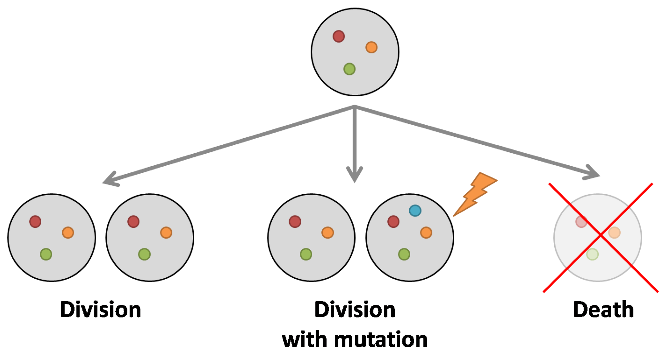
Figure 1. Schematic representation of possible events in the evolution of a population with weakly deleterious mutations. Each large circle represents a single cell, while the smaller colored circles inside them indicate mutations present in that cell. Three types of events are illustrated—left: cell division without additional mutations (number of mutations in parental cell (three) is the same as in progeny cells); middle: cell division with the occurrence of a new mutation (number of mutations in one of the progeny cells increases from 3 to 4); right: cell death event.
Applsci 15 11090 g001
Figure 4. Scatter plots comparing predicted and simulated positions of mutation waves. Predicted values were obtained from numerical solutions to the modified balance equations (Equation (25), cutoff modification, green; Equation (27), exponential modification, blue), while simulated values were generated using the Gillespie algorithm. Each point represents the position of the mutation wave for the deterministic versus stochastic model. It corresponds to a single value of the parameter s, in the range of < 0.0001 ; 0.005 > , and to a time point in the range of < 50 ; 7500 > . The red line in the plot is a reference line that represents the ideal situation in which the results of the deterministic model and the stochastic simulation are identical.
Applsci 15 11090 g004
Figure 5. The plot shows the influence of the value of the parameter α on the average of absolute differences between the predicted and simulated positions of mutation waves (average over 150 time points t k < 50 ; 7500 > ). Values of α were varied in the range of α < 0 ; 4 > . Each of the blue curves corresponds to one value of the weak negative selection coefficient s (in total, 25 values of s < 0.0001 ; 0.005 > ). Black dots indicate the position of the minimum for each curve. The solid orange line represents the median value of the parameter α for the obtained minima, close to 0.12 .
Applsci 15 11090 g005
Figure 6. Comparison of stochastic simulations with deterministic modeling, both without and with modifications of the balance equations. The parameters and layout are the same as in Figure 2. Black solid lines represent the results from the unmodified deterministic system, green lines correspond to the cutoff modification, and blue lines correspond to the exponential modification. Red lines show the stochastic simulations obtained using the Gillespie algorithm.
Applsci 15 11090 g006
Disclaimer/Publisher’s Note: The statements, opinions and data contained in all publications are solely those of the individual author(s) and contributor(s) and not of MDPI and/or the editor(s). MDPI and/or the editor(s) disclaim responsibility for any injury to people or property resulting from any ideas, methods, instructions or products referred to in the content.