Article

On Stability Analysis of Car-Following Models with Various Discrete Operators

Faculty of Computer Science, Bialystok University of Technology, 15-351 Bialystok, Poland
*
Author to whom correspondence should be addressed.
Appl. Sci. 2025, 15(20), 11071; https://doi.org/10.3390/app152011071 (registering DOI)
Submission received: 14 September 2025 / Revised: 10 October 2025 / Accepted: 13 October 2025 / Published: 15 October 2025

Abstract

This paper investigates a car-following model that incorporates both classical and fractional discrete operators. While classical models have been extensively studied, the influence of discrete fractional operators on the stability of such systems has not yet been systematically analyzed. Stability conditions are derived and rigorously proven for systems employing three widely used fractional h-difference operators—Grünwald–Letnikov, Riemann–Liouville, and Caputo—as well as the classical h-difference operator. The analysis reveals that the established conditions are independent of the specific operator used. Furthermore, a comprehensive numerical study validates the theoretical findings and demonstrates that the fractional models can significantly extend the stability bound for the step size from h < 6.67 (classical case) to h < 22.3 (fractional case).

1. Introduction

The car-following model (CFM) describes how a driver adjusts position and speed to follow the vehicle ahead in the same lane [1,2,3]. The concept of CFM originated in 1933 with the work of Greenshields [4,5], who was the first to experimentally investigate traffic flow, density, and speed using photographic measurement techniques. At that time, the term “flow” was not yet established; Greenshields instead referred to “density-vehicles per hour” or “second-kind density.” He proposed a linear relationship between vehicle speed and traffic density. Early research on highway capacity followed two primary approaches: analyzing the speed–density relationship and examining vehicle spacing at high traffic densities. Greenshields’ findings laid the foundation for the development of multi-regime models [6]. Since then, various strategies have emerged to address traffic flow challenges. One prominent approach is the platoon model [7,8,9], where the behavior of vehicles resembles that of a train, with a leading vehicle controlling the motion of the following ones [10]. Another approach is Adaptive Cruise Control (ACC), which enables individual vehicles to autonomously address traffic flow issues. Among these, bilateral control models (BCMs) [11,12,13,14,15,16] stand out, aiming to maintain a vehicle equidistant from both the vehicle ahead and the one behind. Another line of recent research focuses not on individual vehicle behavior, but on optimizing shared mobility systems as a whole. For example, studies on electric vehicle car-sharing platforms explore how scalable infrastructure and dynamic pricing policies can significantly improve system performance, highlighting the role of global design strategies—such as fleet sizing, charger placement, and pricing rules—in enhancing both user satisfaction and economic viability [17,18].
These developments have motivated us to propose a generalized CFM by incorporating fractional operators, offering a novel perspective grounded in fractional calculus, an area of applied mathematics. The integration of fractional operators into CFMs introduces deeper insights into vehicle dynamics. There are several key motivations for this approach. First, memory effects. Classical CFMs often assume instantaneous reactions to changes in the leading vehicle’s behavior. In reality, drivers respond based on past experiences. Fractional calculus captures these memory effects by accounting for the history of vehicle interactions. The next one is that fractional derivatives inherently model non-local behavior, acknowledging that a driver’s reaction depends not only on the current state of the leading vehicle but also on its past behavior. This enhances the model’s realism and improves its ability to capture complex traffic dynamics. Driver behavior also depends on psychology, experience, and anticipation. Fractional calculus provides tools to model these variations, improving the robustness and applicability of CFMs. In summary, applying fractional operators to car-following models offers a more realistic and nuanced representation of traffic dynamics by incorporating memory effects, non-local interactions, and human behavioral complexity. For a comprehensive overview of this field, the reader is referred to [19,20,21,22,23,24,25,26,27].
Previous studies on fractional-order car-following models have primarily considered continuous-time formulations. For instance, Ref. [28] introduced a fractional variant of the classical Pipe’s model, and Ref. [29] proposed a fractional Optimal Velocity Model (FOOV) to incorporate driver memory effects. Later, Ref. [30] extended fractional calculus to macroscopic traffic flow models through local fractional PDEs. More recently, Ref. [31] introduced a fractional-order car-following model with random delay, optimized via an enhanced whale optimization algorithm, further demonstrating the potential of Caputo-based fractional models to enhance stability and robustness under uncertain driving conditions. These works, however, were limited to continuous fractional derivatives, focused on specific operator definitions, and offered only numerical demonstrations of stability rather than general proofs.
In contrast, the present paper is, to the best of our knowledge, the first to conduct a rigorous stability analysis of discrete-time car-following systems involving multiple fractional h-difference operators—namely the Grünwald–Letnikov, Riemann–Liouville, and Caputo operators—alongside the classical discrete operator. The study provides analytically proven sufficient conditions for asymptotic stability that are shown to be independent of the chosen operator, thereby unifying previously fragmented approaches to discrete fractional dynamics. Moreover, by introducing an arbitrary discrete step size h, the authors generalize existing results to encompass digital or sampled implementations, a feature absent in earlier continuous formulations.
Moreover, it is worth noting that fractional-order controllers have been successfully applied to Adaptive Cruise Control (ACC) and cooperative ACC (CACC) systems, demonstrating improved string stability and robustness in vehicle platoons [32,33]. In particular, the Grünwald–Letnikov fractional PID (GL-PID) has been shown to outperform classical PID controllers by delivering smoother acceleration/deceleration profiles and better disturbance rejection in realistic driving scenarios [34]. These results reinforce the potential of discrete fractional models like ours to be deployed in automated vehicle control frameworks and intelligent transportation systems.
Our numerical experiments demonstrate that the proposed fractional-order discrete models significantly extend the stability region compared with the classical model (e.g., from h < 6.7 in the integer case to h < 22.3 for α = 0.5), and that among the fractional formulations, the Caputo operator yields the most physically realistic vehicle responses. Such a comparative evaluation of multiple discrete fractional operators within a car-following context has not been reported previously. We explore the application of Grünwald–Letnikov, Riemann–Liouville, and Caputo fractional h-difference operators to classical CFMs. Our goal is to determine whether these modifications enhance model stability. Specifically, we assess whether stability can be achieved in cases where the classical model is unstable, and whether fractional operators accelerate convergence in cases where the classical model is already stable.
The key contributions of this paper that advances the literature are summarized as follows:
  • use of fractional operators to capture memory effects and non-local interactions;
  • derivation of system stability conditions involving the three principal fractional-order operators: Grünwald–Letnikov, Riemann–Liouville, and Caputo, together with the classical case;
  • incorporation of models with an arbitrary step size h, aligning more closely with real-world applications;
  • establishing rigorous, operator-independent stability criteria for fractional discrete CFMs;
  • integrating three fractional operator definitions in a unified discrete framework;
  • demonstrating, both analytically and numerically, the superior stability and implementation potential of fractional-order discrete models—particularly those based on the Caputo operator—over classical integer-order formulations.
The paper is structured as follows. The symbols used are listed in Table 1. In the Section 2, we introduce the necessary definitions and foundational results. Section 3 presents the proposed model and our main theoretical findings. In particular, we provide theorems establishing sufficient conditions for the asymptotic stability of CFMs with fractional operators Grünwald–Letnikov, Riemann–Liouville, and Caputo, together with the classical operator—equivalent to the stability of the original systems. Additionally, in the last section, we provide extensive simulations that demonstrate the impact of fractional operators on system behavior, covering both stable and unstable classical model scenarios. These examples not only validate our theoretical findings but also enable a comparative analysis of the operators’ effects.
To highlight the contribution of this work in the context of existing research, Table 2 summarizes several representative studies on car-following and fractional-order models, indicating their main focus and the research gaps addressed by the present paper.
For the convenience of the reader we present a diagram summarizing the methodological workflow used in the article (see Figure 1).

2. Preliminaries

Let α > 0 . We define the following sequence:
a ( α ) ( k ) : = 1 f o r k = 0 ( 1 ) k α ( α 1 ) ( α k + 1 ) k ! f o r k N .
Note that a ( α ) ( k ) can also be defined in the recurrence way by the following:
a ( α ) ( 0 ) : = 1 , a ( α ) ( k + 1 ) : = 1 α + 1 k + 1 a ( α ) ( k ) , k N 0 .
Definition 1
([35]). Let h > 0 . For a function x : ( h N ) 0 R the forward h-difference operator is defined as
Δ h x ( k h ) : = x ( ( k + 1 ) h ) x ( k h ) h .
Let q N and Δ h q : = Δ h Δ h q t i m e s be q-fold application of operator Δ h , i.e.,
Δ h q x = Δ h Δ h Δ h x q t i m e s
and we write Δ h 0 x ( k h ) : = x ( k h ) .
Using the sequence (2) one can define the following difference operator.
Definition 2
([35]). For a function x : ( h N ) 0 R the fractional h-sum of order α > 0 is given by
Δ h α x k h : = h α i = 0 k a ( α ) ( k i ) x ( i h ) ,
where k N 0 .
Henceforth, we confine our analysis to the case α ( 0 , 1 ] .
Definition 3
([35]). Let α ( 0 , 1 ] . The Grünwald–Letnikov fractional h-difference operator Δ h α G L of order α for a function x : ( h N ) 0 R is defined by
Δ h α G L x ( k h ) : = h α i = 0 k a ( α ) ( i ) x ( ( k i ) h ) ,
where a ( α ) ( i ) i N 0 is the sequence given by (2) or equivalently, by (1).
Observe that, for α = 0 and h = 1 we have Δ h α G L x ( k ) = x ( k ) and for α = 1 we get Δ h α G L x ( k ) : = x ( k ) x ( k 1 ) .
Definition 4
([35]). Let α ( 0 , 1 ] . The Riemann–Liouville fractional h-difference operator Δ h α R L of order α for a function x : ( h N ) 0 R is defined by
Δ h α R L x ( k h ) : = Δ h Δ h α 1 x ( k h ) .
Remark 1
(cf. [35]). The Riemann–Liouville and Grünwald–Letnikov fractional h-difference operators are equivalent.
Definition 5
([35]). Let α ( 0 , 1 ] . The Caputo fractional h-difference operator Δ h α C of order α for a function x : ( h N ) 0 R is defined by
Δ h α C x ( k h ) : = Δ h α 1 Δ h x ( k h ) .
Let us consider linear system with Riemann–Liouville fractional h-difference operator
Δ h α R L x ( k h ) = A x ( k h ) ,
where A R n × n .
Remark 2
(cf. [37]). For the scalar system A = λ < 0 and α ( 0 , 1 ] we have, it is asymptotically stable if and only if | λ | < 2 h α .
Remark 3
([37]). There is a possibility to have asymptotic stability if λ = 0 S p e c ( A ) , when zero eigenvalue is singular.
Now let us consider a linear system with the Caputo fractional h-difference operator.
Δ h α C x ( k h ) = A x ( k h ) ,
where A R n × n .
Proposition 1
(cf. [35]). Systems (8) or (9), with α ( 0 , 1 ] are asymptotically stable if and only if both conditions are satisfied
1. 
There is k N 0 such that
arg λ i [ a , b ] ,
where a = 2 π frac { α ( k + 1 4 ) } , b = 2 π ( 1 frac { α ( 1 4 k ) } ) and frac { x } : = x x .
2. 
For all i = 1 , , n and k , s Z
| λ i | < 2 h s i n arg λ i α π 2 2 ( β k + s ) π 2 α α , i = 1 , , n ,
where arg λ i and | λ i | are, respectively, the main argument and modulus of λ i S p e c ( A ) .
Remark 4
(cf. [36]). Let λ R . Then system (9) takes the following form
Δ h α C ( k h ) = λ x ( k h ) ,
where α ( 0 , 1 ] . If
2 h α < λ < 0 .
then Equation (10) is asymptotically stable.

3. Car-Following Model

We start our investigation with the classical continuous-time framework, and consider n autonomous vehicles in a car-following system, where i-th vehicle follows the ( i 1 ) -th vehicle. The dynamics of the system are considered by modeling the position of the i-th vehicle at time t as x i ( t ) , with its velocity defined as v i ( t ) = x ˙ i ( t ) . The pair { x i ( t ) , v i ( t ) } defines the full state of vehicle i. The vehicle’s behavior is modulated through its acceleration v ˙ i ( t ) = x ¨ i ( t ) , which is determined by a control mechanism. In the context of the car-following model, the acceleration is modeled as follows:
v ˙ i = k d ( x i 1 x i s ) + k v ( v i 1 v i ) ,
where s represents the desired inter-vehicle spacing, commonly referred to as the safe distance. The parameters k d > 0 and k v > 0 are control gains associated with position and velocity feedback, respectively. This formulation implies that each vehicle adjusts its motion based solely on the relative distance and relative speed to the vehicle immediately ahead. In ideal conditions, all vehicles maintain the safe distance s from one another and travel at a constant speed v 0 . In such a configuration, the system is at equilibrium, with all accelerations v ˙ i equal to zero.
One can consider a discrete-time system, accordingly, based on a discretized formulation of the dynamics. Then Equation (11) gets the form
Δ h v i ( k ) = k d ( x i 1 ( k ) x i ( k ) s ) + k v ( v i 1 ( k ) v i ( k ) ) ,
where Δ h is h-difference operator, Δ h v i ( k ) : = v i ( k + h ) v i ( k ) h .
Further, assuming that the velocity of the first, leading car remains constant, the system of dynamics for the first vehicle can be written as
x 1 ( k + h ) = x 1 ( k ) + h v 1 ( k ) v 1 ( k + h ) = v 1 ( k )
while that for the rest of the vehicles is as follows:
x i ( k + h ) = x i ( k ) + h v i ( k ) v i ( k + h ) = k d h ( x i 1 ( k ) x i ( k ) s ) + k v h ( v i 1 ( k ) v i ( k ) ) + v i ( k ) f o r   i = 2 , , n .
Then the pair { x i ( k ) , v i ( k ) } is the state of the i-th car, where x i ( k ) is the position of i-th car and v i ( k ) is its velocity at the moment k. For Y i ( k ) = x i ( k ) v i ( k ) , let Y ( k ) = ( Y 1 ( k ) , , Y n ( k ) ) T be the state vector containing the states of all cars in the traffic system at the moment k. Subsequently, a linear system of the general form is considered:
Δ h Y ( k ) = A Y ( k ) ,
where k d > 0 is the proportional gain, k v > 0 is the derivative gain, h > 0 is the step size, k N 0 , and
A = 0 1 0 0 0 0 0 0 0 0 0 0 0 0 0 1 0 0 k d k v k d k v 0 0 0 0 0 0 0 1 0 0 k d k v k d k v R 2 n × 2 n .
Observe that the second row of matrix A is composed entirely of zeros. This arises from the fact that we assume that the velocity of the first, leading vehicle remains constant, i.e., v 1 ( k + h ) = v 1 ( k ) , for all moments of k. Consequently, the acceleration of the leading vehicle is zero, reflecting the absence of any change in its velocity.
Next, system (13) can then be written in discrete matrix form as follows:
Y ( k + h ) = ( I + h A ) Y ( k ) ,
where matrix A is given by (14).

3.1. Car-Following Model with Fractional h-Difference Operators

In this section, our investigation centers on three of the most well-known fractional operators: Grünwald–Letnikov, Riemann–Liouville, and Caputo. We examine the stability of the system and derive sufficient conditions under which stability is guaranteed. For this purpose, let us discretize the model given by (11) using fractional h-difference operators. We consider a linear system in the following general form:
Δ h α Y ( k h ) = A Y ( k h ) ,
where Δ h α is the Grünwald–Letnikov Δ h α G L , Caputo Δ h α C , or Riemann–Liouville Δ h α R L fractional h-difference operator, k d > 0 is the proportional gain, k v > 0 is the derivative gain, h > 0 is the step size, α ( 0 , 1 ] , k N 0 , and matrix A is given by (14).
To investigate the stability problem of system (16), let us consider the transformation of this system as follows:
x ¯ i 1 = x i x 1 , v ¯ i 1 = v i v 1 , i = 2 , , n .
Then, system (16) can be written as
Δ h α Y ¯ ( k h ) = A ¯ Y ¯ ( k h ) ,
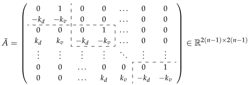
where Y ¯ = ( Y ¯ 1 , , Y ¯ n 1 ) T , Y ¯ i ( k ) = x ¯ i ( k ) v ¯ i ( k ) , i = 1 , , n 1 and
Applsci 15 11071 i001
Observe that the discrete form of system (18) with Riemann–Liouville fractional h-difference operator is the following:
Y ¯ ( ( k + 1 ) h ) = ( h α A ¯ + α I ) Y ¯ ( k h ) i = 2 k + 1 a ( α ) ( i ) Y ¯ ( ( k i + 1 ) h )
and with Caputo fractional h-difference operator it is
Y ¯ ( k h ) = ( I + h α A ¯ ) Y ¯ ( k 1 ) h i = 1 k 1 a ( α 1 ) ( k i ) Y ¯ ( i h ) Y ¯ ( ( i 1 ) h ) .
Lemma 1.
For matrix A ¯ defined by (19) it holds
S p e c ( A ¯ ) = k v k v 2 4 k d 2 ( n 1 ) times , k v + k v 2 4 k d 2 ( n 1 ) times .
Proof. 
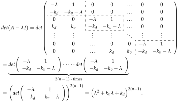
Let us observe that matrix A ¯ is a lower triangular block matrix. Using this fact, one gets
Applsci 15 11071 i002
Thus
S p e c ( A ¯ ) = k v k v 2 4 k d 2 ( n 1 ) times , k v + k v 2 4 k d 2 ( n 1 ) times .
Subsequently, we can provide the sufficient condition for the stability of system (18).
Theorem 1.
Let us consider system (18). If one of the following assumptions holds as follows:
1. 
k v 2 4 k d , 2 α + 1 h α < k v ± k v 2 4 k d < 0 for k v , k d , h > 0 , α ( 0 , 1 ] ,
2. 
k v 2 < 4 k d , k d < 2 h sin arg λ α π 2 2 α 2 α for λ S p e c ( A ¯ ) , k v , k d , h > 0 , α ( 0 , 1 ] ,
then system (18) is asymptotically stable.
Proof. 
First, let us consider the case when k v 2 4 k d . Along with the assumption 2 α + 1 h α < k v ± k v 2 4 k d < 0 , one gets 2 α h α < k v ± k v 2 4 k d 2 < 0 , for k v , k d , h > 0 . By Lemma 1, λ S p e c ( A ¯ ) is equal to λ = k v + k v 2 4 k d 2 or λ = k v k v 2 4 k d 2 . It follows that for any λ S p e c ( A ¯ ) one gets | λ | < 2 h α and by Remarks 1, 2, and 4, system (18) is asymptotically stable.
Next, let us assume that k v 2 < 4 k d . Then, according to Lemma 1, λ S p e c ( A ¯ ) is equal to λ = k v 2 + j 4 k d k v 2 2 or λ = k v 2 j 4 k d k v 2 2 . We observe that for α ( 0 , 1 ] , it follows that 3 π 2 2 π α π 2 < 2 π . If λ = k v 2 + j 4 k d k v 2 2 , then one gets φ = a r c t a n 4 k d k v 2 k v and since φ lies in the second quadrant, the main argument is a r g λ = π a r c t a n 4 k d k v 2 k v π 2 , π . Using the previous observation, it can be limited to a r g λ α π 2 , 2 π α π 2 . Similarly, for λ = k v 2 j 4 k d k v 2 2 , one gets a r g λ = π + a r c t a n 4 k d k v 2 k v π , 3 π 2 α π 2 , 2 π α π 2 . Hence, arg λ α π 2 , 2 π α π 2 for each λ S p e c ( A ¯ ) and condition 1 in Proposition 1 is fulfilled with k = 0 . In addition, observe that | λ | = k d for every λ S p e c ( A ¯ ) . By assumptions we obtain | λ | < 2 h sin arg λ α π 2 2 α α , which means that condition 2 in Proposition 1 is satisfied with k = s = 0 . Hence, by Proposition 1 and Remark 1 it follows that system (18) is asymptotically stable. □
The asymptotic stability of system (18) implies v i v 1 and x i x 1 , i = 2 , , n . However, in physical systems, to prevent collisions, a safe distance s is maintained. This constraint leads to the modified condition that the positions of the vehicles approach x i x 1 + i × s for i = 2 , , n , thereby ensuring the necessary separation between the vehicles. Once system (18) reaches stability, all vehicles move with a uniform velocity v 1 .

3.2. Car-Following Model—Classical Case

In this subsection, we focus on the classical discretized car-following model given as follows:
Δ h Y ( k ) = A Y ( k )
where Y = ( Y 1 , , Y n ) T is the state vector that contains the states of all cars in the traffic system with Y i ( k ) = x i ( k ) v i ( k ) where x i ( k ) is the position of the i-th car and v i ( k ) is its velocity at the moment k and matrix A is given by (14).
Again, to investigate stability, we use the transformation
x ¯ i 1 = x i x 1 , v ¯ i 1 = v i v 1 , i = 2 , , n .
Then system (22) with step h > 0 can be rewritten as
Y ¯ ( k + h ) = ( I + h A ¯ ) Y ¯ ( k ) .
where A ¯ R 2 ( n 1 ) × 2 ( n 1 ) is given by (19).
Let us recall the classical fact on asymptotic stability for discrete-time systems.
Proposition 2
([38]). A discrete-time system x ( k + 1 ) = A x ( k ) is asymptotically stable if and only if the matrix A is a Schur matrix, i.e., all eigenvalues λ of A satisfy | λ | < 1 .
Theorem 2.
Let us consider system (24). If one of the following assumptions holds,
1. 
k v 2 4 k d , 4 h < k v k v 2 4 k d < 0 ,
2. 
k v 2 < 4 k d , k d < k v h ,
then system (24) is asymptotically stable.
Proof. 
First, consider the case where k v 2 4 k d . By Lemma 1 and basic algebraic properties it follows that
S p e c ( I + h A ¯ ) = 1 + h k v k v 2 4 k d 2 ( n 1 ) times , 1 + h k v + k v 2 4 k d 2 ( n 1 ) times , which together with the assumption 4 h < k v k v 2 4 k d < 0 implies that | λ | < 1 for each λ S p e c ( I + h A ¯ ) and system (24) is asymptotically stable.
Next, consider k v 2 < 4 k d . Then using, again, Lemma 1 and basic algebraic properties, we get S p e c ( I + h A ¯ ) = 1 + h k v j 4 k d k v 2 2 ( n 1 ) times , 1 + h k v + j 4 k d k v 2 2 ( n 1 ) times . Observe that | λ | = 1 h k v + h 2 k d for every λ S p e c ( I + h A ¯ ) . By assumption k d < k v h , we obtain 1 h k v + h 2 k d < 1 , which implies that the matrix ( I + h A ¯ ) is a Schur matrix. Hence, by Proposition 2, system (24) is asymptotically stable. □

4. Numerical Simulations

This section presents numerical simulations that illustrate and validate the theoretical results discussed earlier. Various scenarios are analyzed to demonstrate the stability properties of classical and fractional-order models under different parameter settings.
Example 1.
Consider a scenario involving n = 4 vehicles with randomly selected initial conditions given by Y ( 0 ) = [ 7 , 2 , 6 , 1 , 4 , 3 , 2 , 4 ] . The control gains are set to k d = 0.06 and k v = 0.5 . To prevent collisions between vehicles, a safety distance of s = 2 was enforced during the simulations.
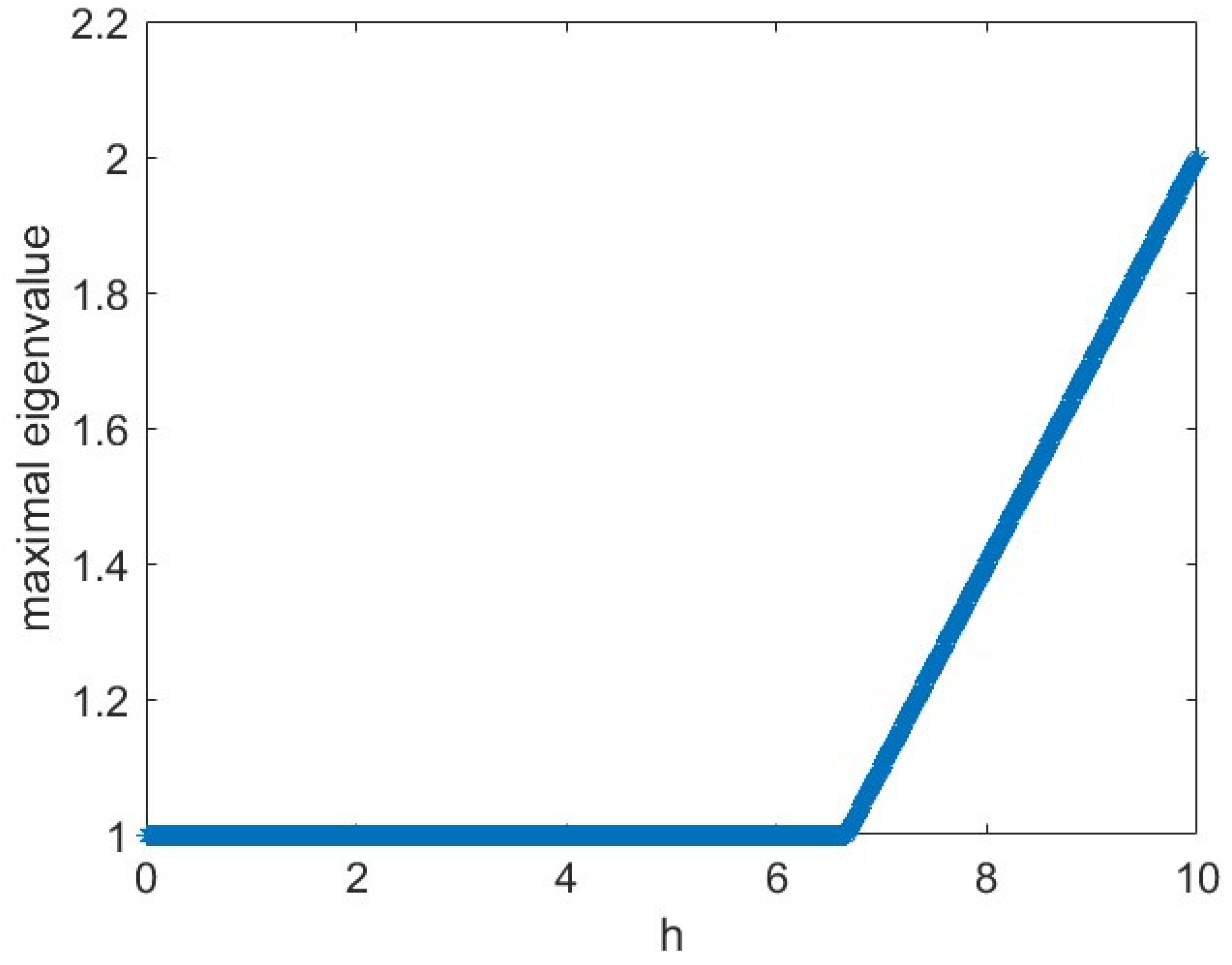
Figure 2 illustrates the dependence of the eigenvalues of system (22) as a function of the discretization step h. The results indicate that the classical model remains stable for step sizes smaller than approximately h = 6.7 . Note that for k d = 0.06 and k v = 0.5 the assumption 1 of Theorem 2 is satisfied. Based on condition 1 of Theorem 2, and given that the specified values of k d and k v yield real eigenvalues, the theoretical stability condition imposes an upper bound of h < 6.67 .
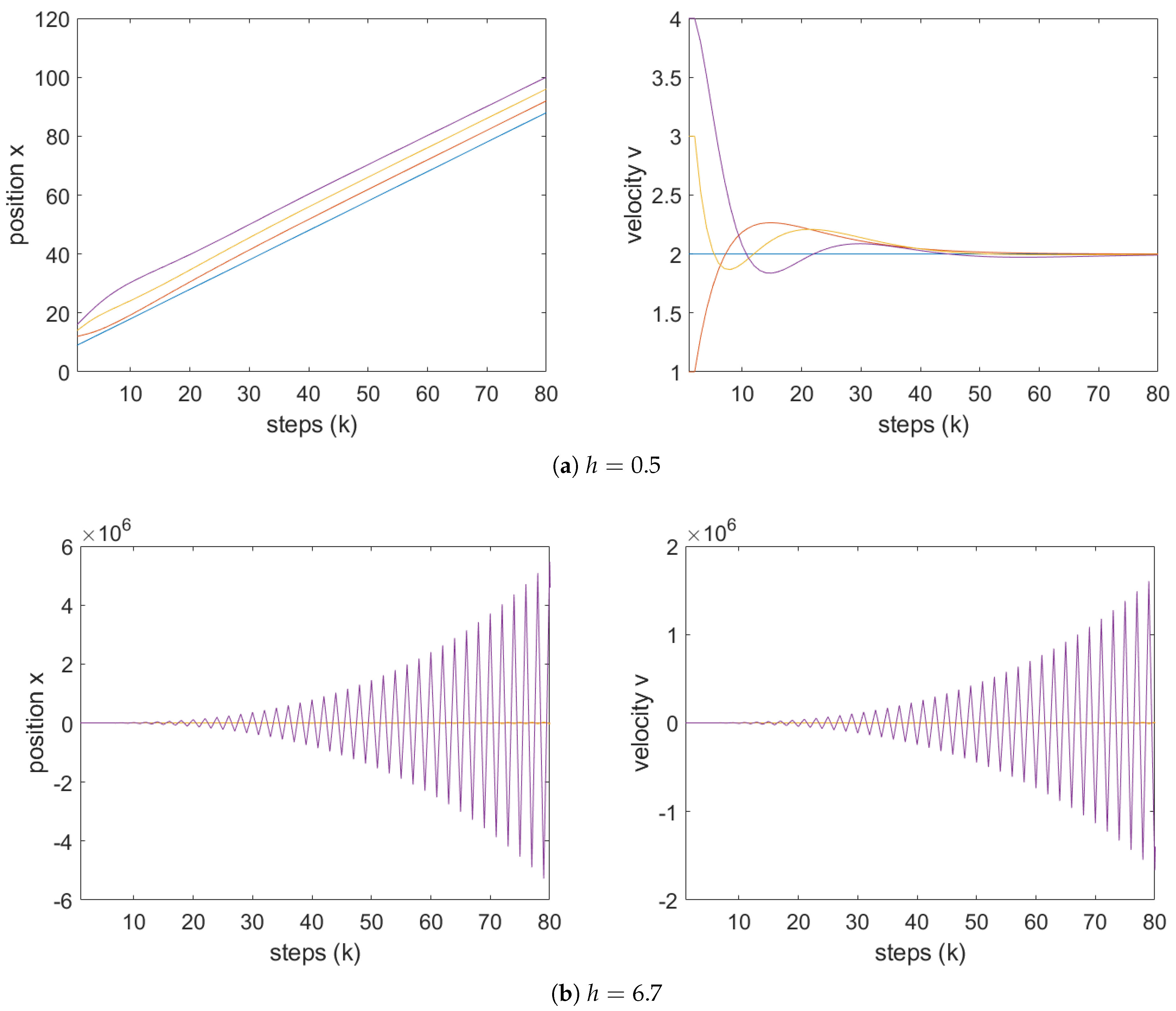
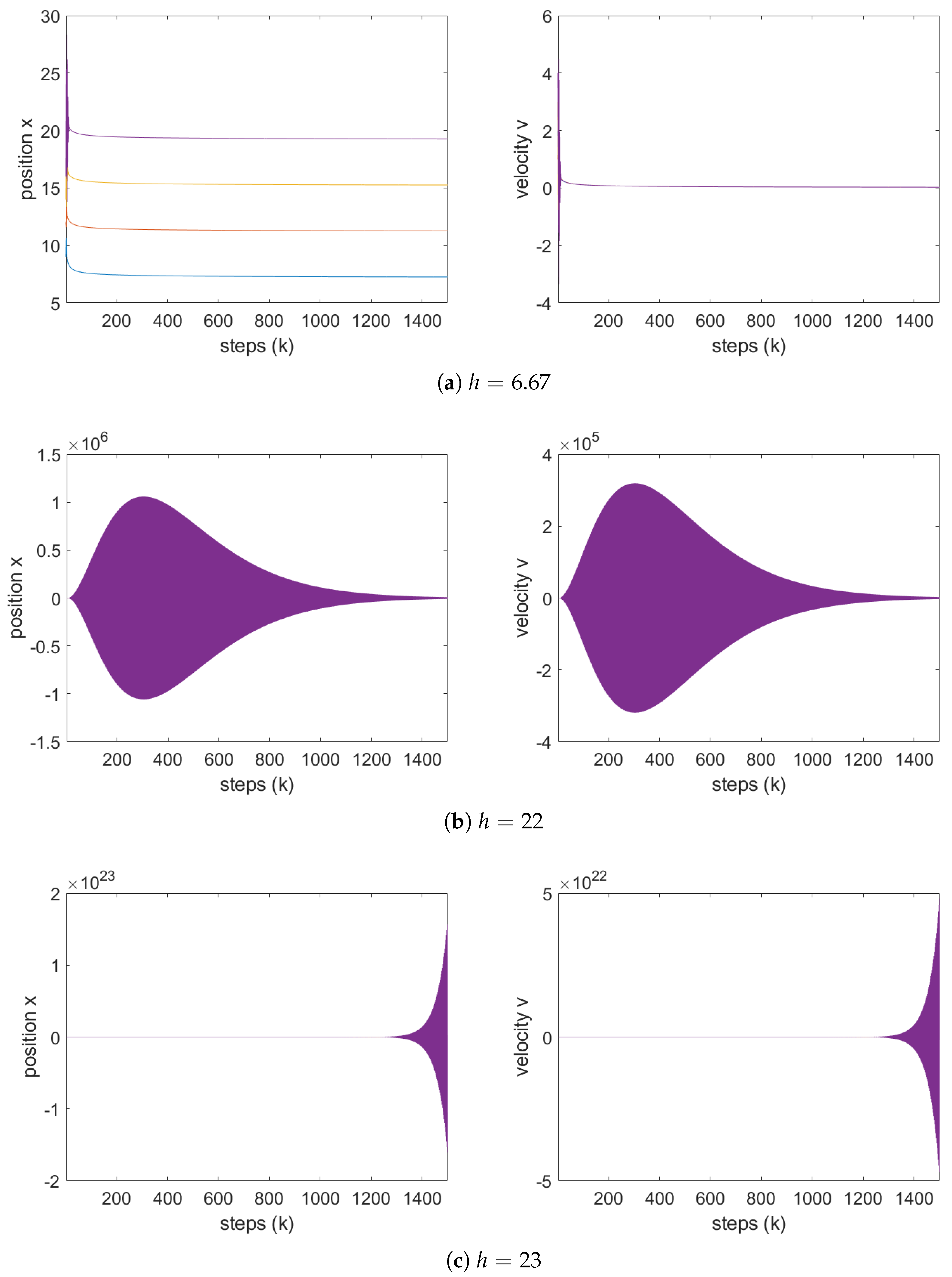
This analytical result is supported by numerical simulations. Figure 3 presents the evolution of the positions and velocities of the vehicles for selected values of h in the classical model. When the step size exceeds the theoretical bound (e.g., h = 6.7 ), the system becomes unstable, as evidenced by the lack of convergence of vehicle velocities to that of the leader and the absence of coordinated, parallel motion.
Next, we fix the step size h = 1 and analyze the system behavior for various values of α ( 0 , 1 ] . Observe that for k d = 0.06 and k v = 0.5 the assumption 1 of Theorem 1 is satisfied. According to condition 1 of Theorem 1, a system incorporating a fractional h-difference operator remains stable for any α within this interval. The stability condition from the theorem reduces in this case to the following: 2 α + 1 < 0.5 which clearly holds for all α ( 0 , 1 ] .
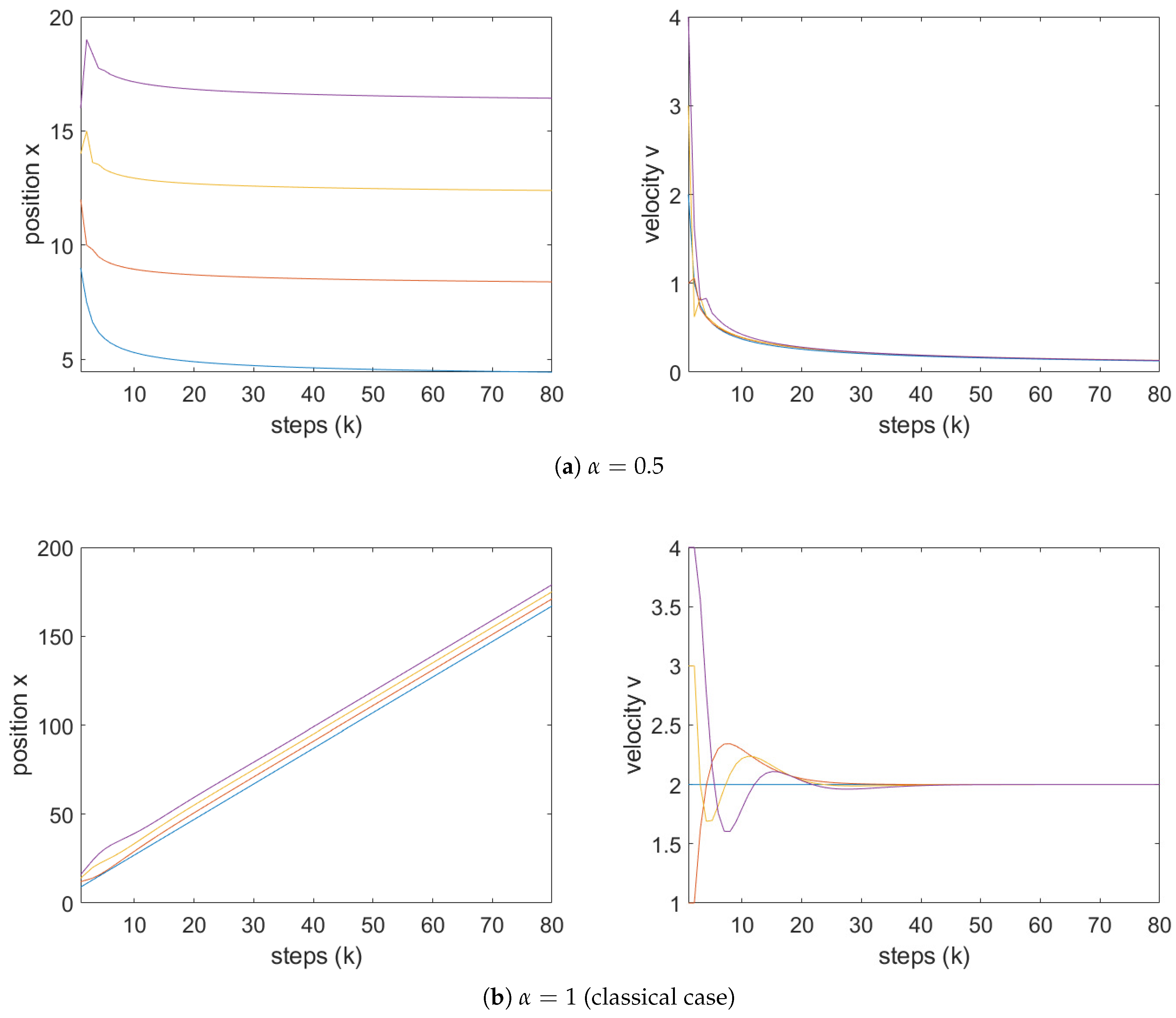
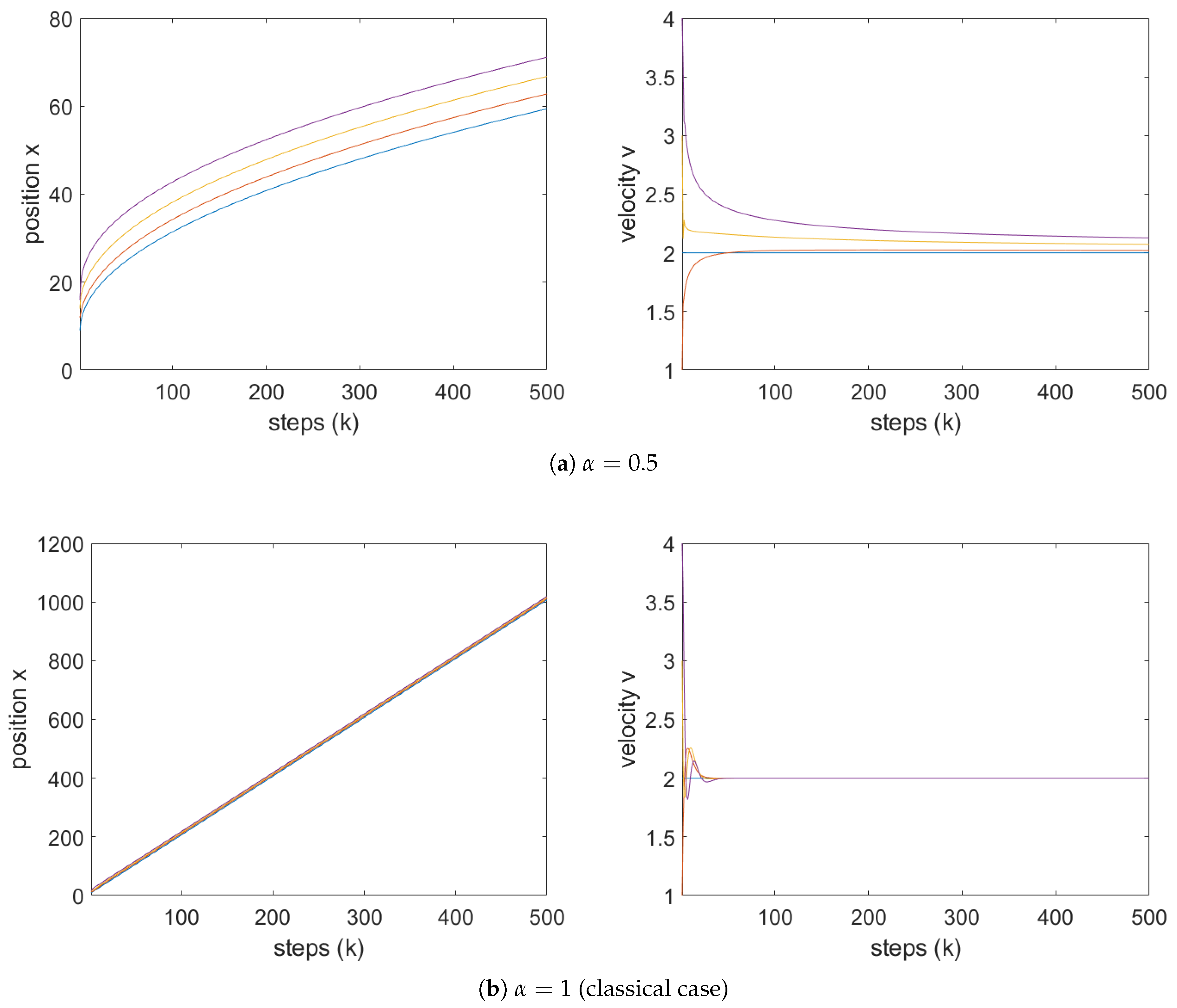
Figure 4 and Figure 5 present numerical simulations of vehicle positions and velocities for models employing the Grünwald–Letnikov and Caputo fractional differential operators, respectively, with h = 1 . In agreement with the theoretical analysis, both models exhibit convergence for any α ( 0 , 1 ] .
As α 1 , the models approach the classical case. However, for small values of α , the system governed by the Grünwald–Letnikov operator tends to drive vehicle velocities toward zero—a behavior that is undesirable in practical applications. In contrast, although the Caputo-based model converges slightly more slowly, it avoids this degradation in velocity, rendering it more suitable for real-world implementations.
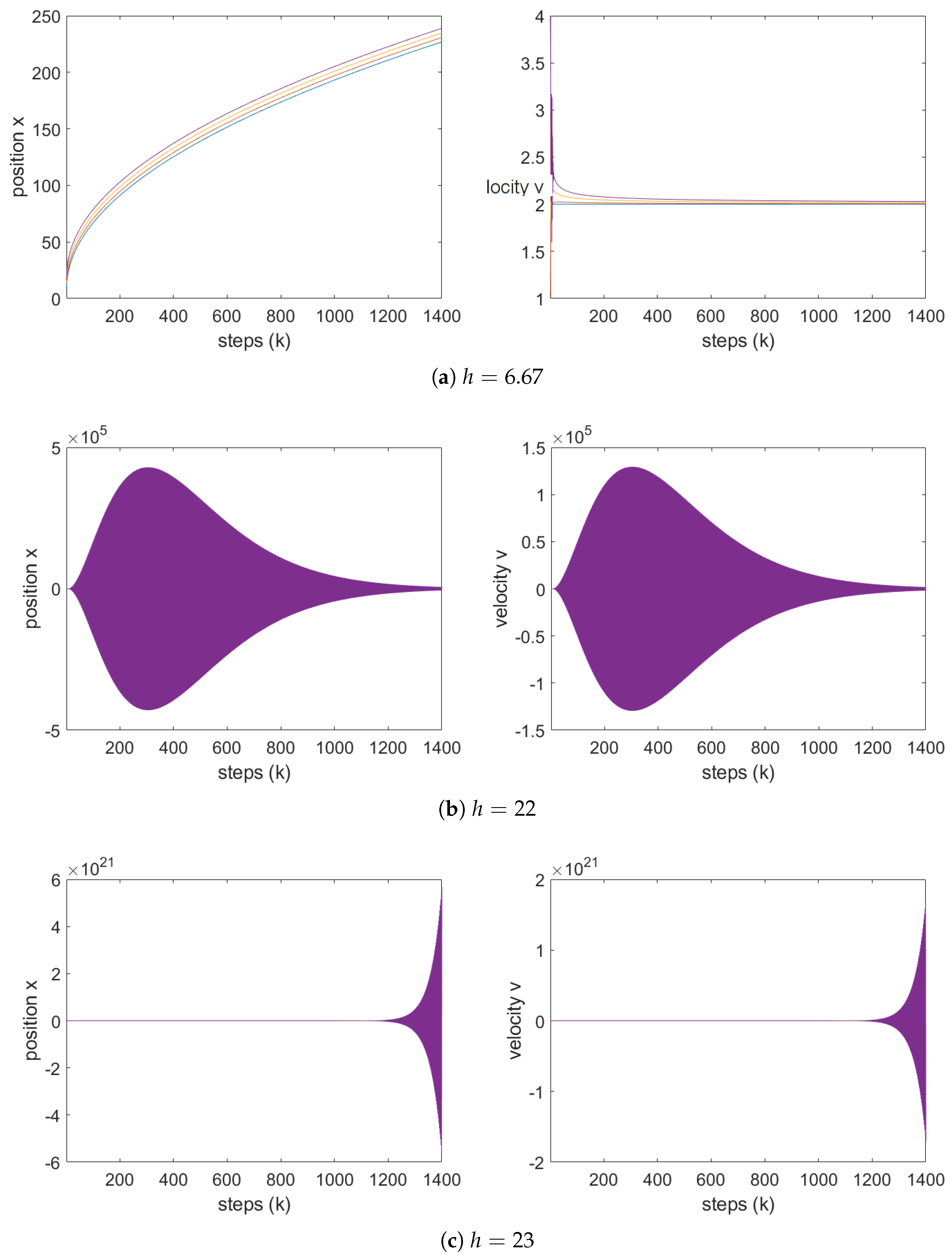
To further investigate the influence of step size, we fix α = 0.5 and perform simulations for varying values of h in both fractional models. The results are shown in Figure 6 and Figure 7. According to point 1 of Theorem 1, the stability condition in this case becomes the following: 2 1.5 h 0.5 < 0.6 , which leads to the constraint h < 22.3 . Notably, this represents a significant improvement compared to the classical model, where stability is only ensured for h < 6.67 . These calculations are fully supported by the numerical results shown in Figure 6 and Figure 7, corresponding to the Grünwald–Letnikov and Caputo operators, respectively.
Example 2.
Consider n = 4 vehicles, using the same initial conditions as before, Y ( 0 ) = [ 7 , 2 , 6 , 1 , 4 , 3 , 2 , 4 ] , but with control gains set to k d = 0.18 and k v = 0.1 . The safety distance is again assumed to be s = 2 .
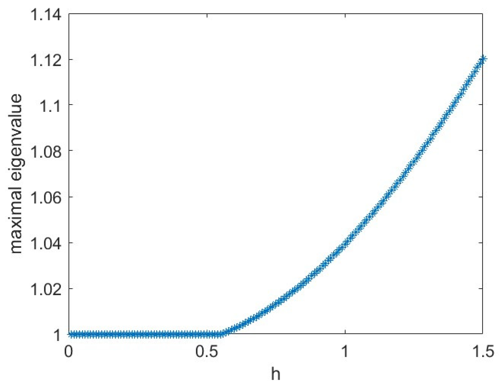
Observe that for k d = 0.18 and k v = 0.1 the assumption 2 of Theorem 2 is satisfied. The chosen parameter values lead to complex eigenvalues of system (22). Consequently, point 2 of Theorem 2 can be used to determine the range of the step size h for which the classical model remains stable. Specifically, the condition 0.18 < 0.1 h leads to the bound h < 0.556 .
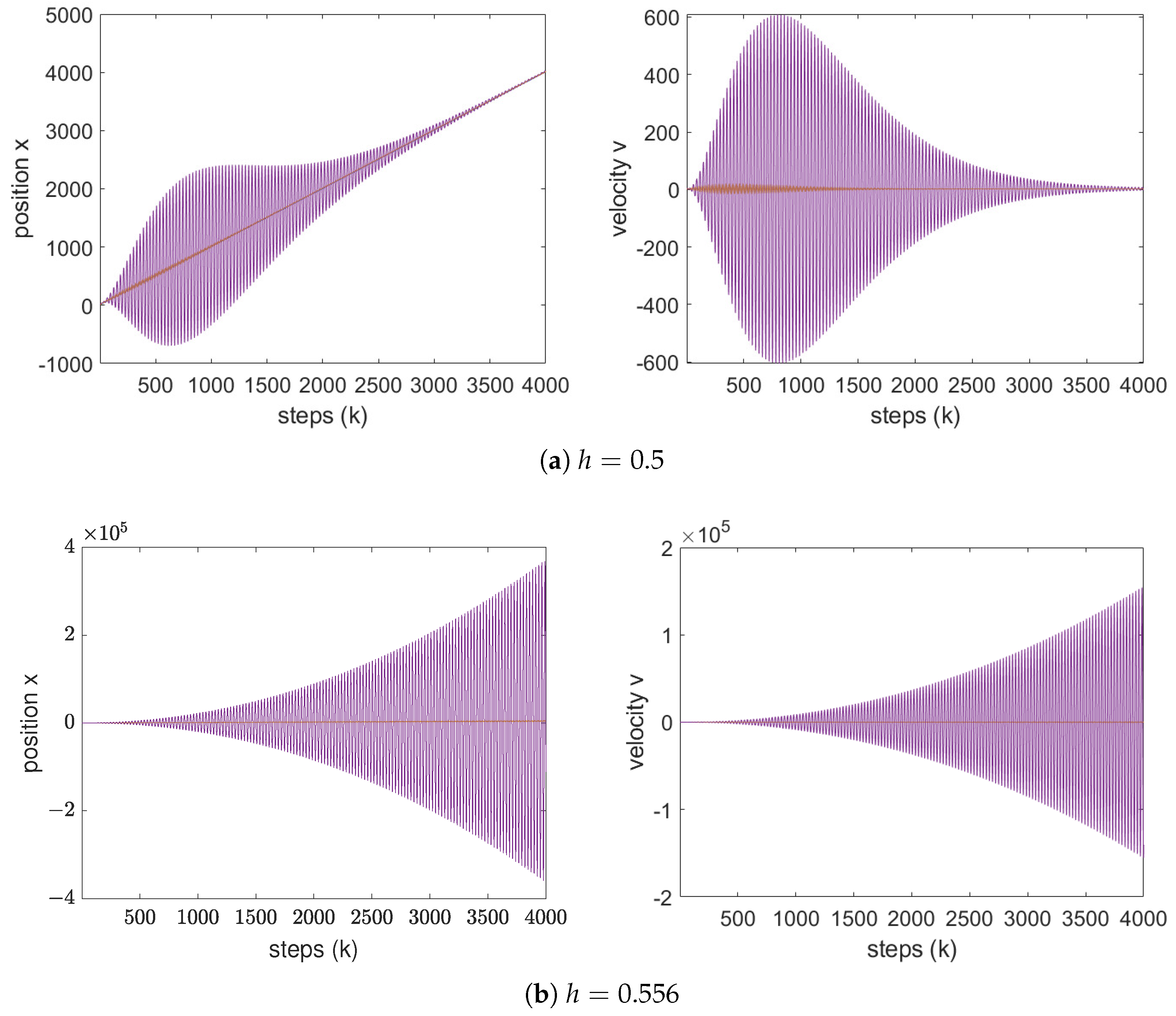
This calculation is confirmed by the simulation results presented in Figure 8, which shows the maximum real part of the eigenvalues of the classical system as a function of h. Further confirmation is provided by the time-domain simulations of vehicle positions and velocities for the given parameters in the classical model, shown in Figure 9. For step sizes h 0.556 , the vehicle velocities no longer converge to that of the leader, indicating instability.
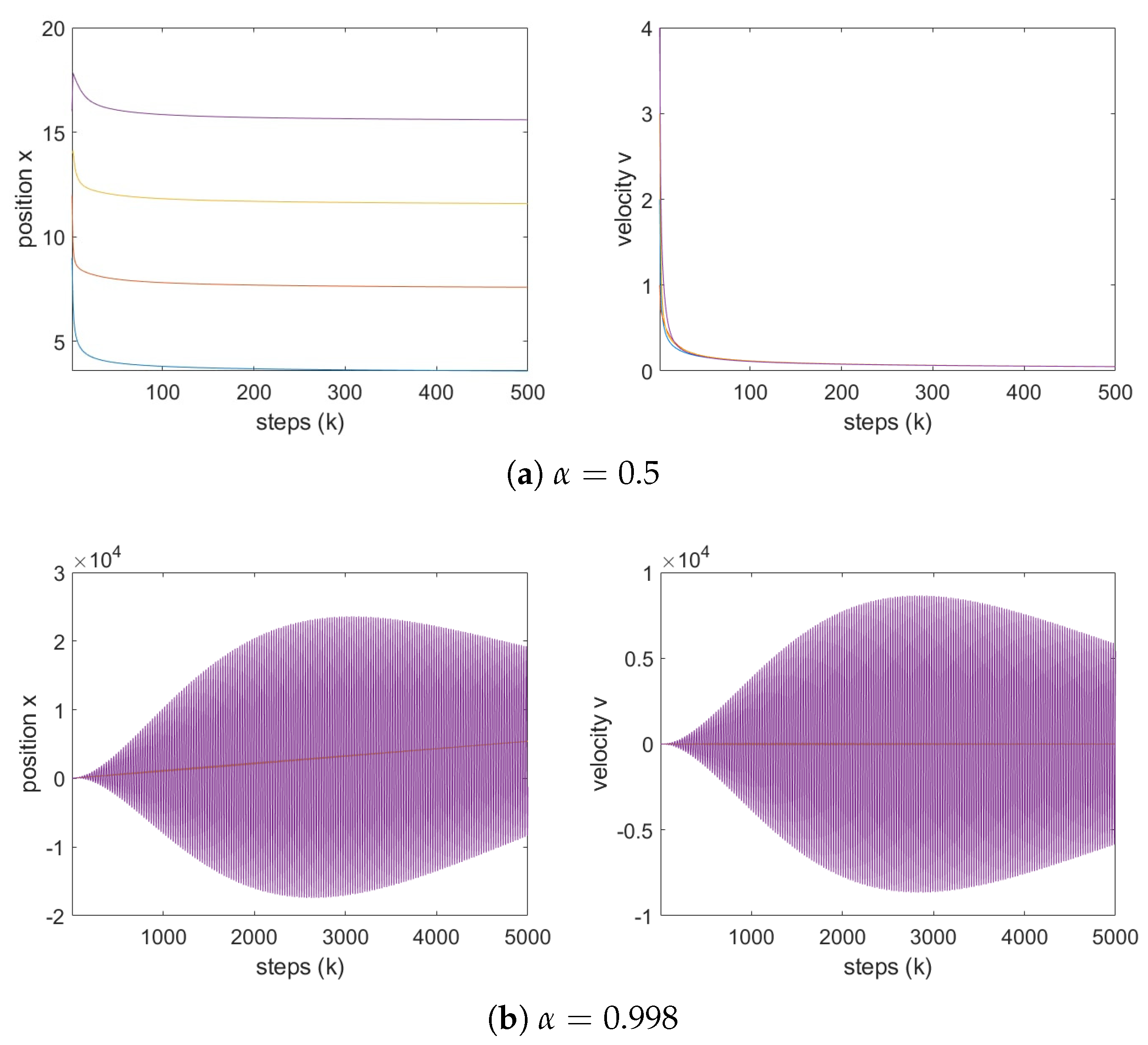
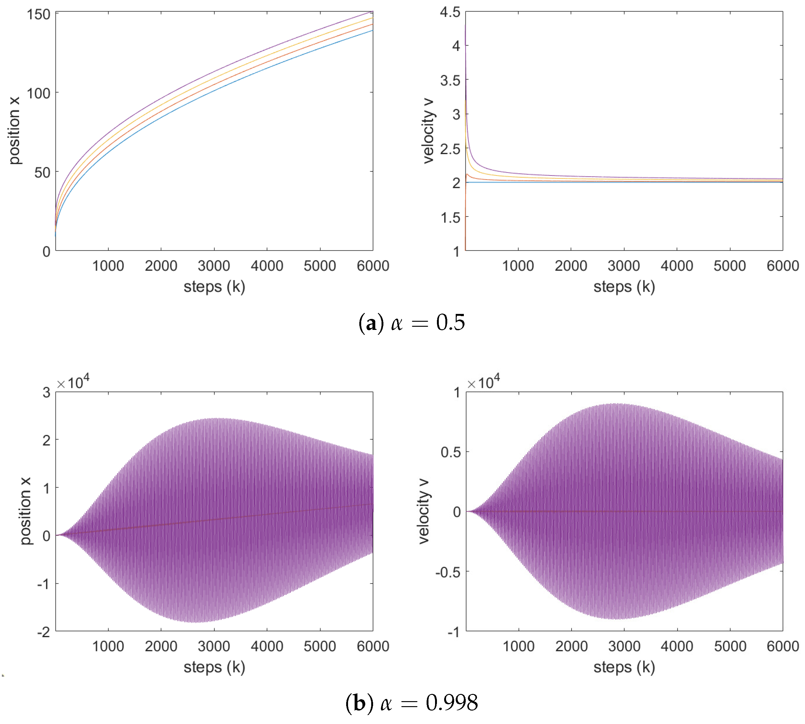
Now, fix h = 0.556 , for which the classical model becomes unstable when using the gains k d = 0.18 and k v = 0.1 . Figure 10 and Figure 11 illustrate the system’s behavior under the Grünwald–Letnikov and Caputo fractional differential operators, respectively, for h = 0.556 and several values of α ( 0 , 1 ] .
As observed from the simulations, both fractional-order models maintain stability for α 0.998 . Observe that for k d = 0.18 and k v = 0.1 the assumption 2 of Theorem 1 is satisfied. The obtained result is consistent with Theorem 1. The eigenvalues of the system are given by λ 1 = 0.05 + 0.4213 j and λ 2 = 0.05 0.4213 j , with corresponding arguments arg ( λ 1 ) = 0.537 π and arg ( λ 2 ) = 0.537 π . For α = 0.998 , condition 2 in Theorem 1 leads to the following inequality:
k d < 2 0.556 sin ± 0.537 π 0.998 π 2 2 0.998 2 · 0.998 .
These yield bound k d < 0.1808 . Since the chosen gain k d = 0.18 satisfies inequality, the system remains stable under the corresponding condition.
It is worth noting that for α = 1 , the model reduces to the classical (integer-order) case, which is unstable in this configuration. Therefore, the application of fractional-order differential operators significantly enhances the stability of the system.
Remark 5.
It should be noted that all simulations presented in this study are based on synthetic data. This approach allows full control of system parameters and facilitates direct validation of the theoretical stability conditions. Nevertheless, the developed framework could also be applied to real-world vehicle trajectory datasets, such as NGSIM or HighD, which provide high-resolution measurements of car-following behavior under natural driving conditions. In future studies, the proposed framework could be calibrated and validated using such datasets to further assess its realism and practical applicability.

5. Conclusions

This article focused on the analysis of a car-following model enhanced with fractional- and integer-order dynamics. Specifically, the Grünwald–Letnikov, Riemann–Liouville, and Caputo fractional as well as classical h-difference operators were incorporated into the model to investigate the stability of the considered systems.
For the first time, sufficient stability conditions for the car-following model employing each of the mentioned fractional operators were formulated and rigorously proved. The theoretical results were complemented by extensive numerical simulations, which provided illustrative comparisons between the fractional and classical formulations.
The simulation results confirmed that the use of fractional-order operators can substantially extend the admissible discretization step size and improve the stability properties of the system. In particular, the Caputo operator demonstrated favorable characteristics for practical applications, avoiding undesired behaviors such as velocity decay observed in other formulations.
From a practical perspective, the observed differences between the Grünwald–Letnikov and Caputo formulations may have important implications for real-world control systems such as Adaptive Cruise Control (ACC) and Connected Autonomous Vehicles (CAVs). The smoother convergence behavior of the Caputo-based model suggests that it may provide greater robustness against abrupt changes in leader velocity and better comfort for passengers—both key requirements in automated driving. In contrast, the Grünwald–Letnikov formulation, while theoretically valid and faster to converge, can produce overly aggressive corrections or excessive damping, which may be undesirable in practical implementations. Therefore, fractional models based on the Caputo operator appear more suitable for control-oriented applications in intelligent transportation systems.
These findings support the relevance and effectiveness of fractional calculus in improving the performance and robustness of car-following models and open new avenues for its application in traffic flow analysis and control. Future research could focus on several directions that naturally extend the present work. First, stochastic formulations of the fractional car-following model could be developed to account for variability and uncertainty in driver behavior. Another promising avenue involves the extension of the current single-lane framework to multi-lane, enabling the study of lane-changing interactions and collective dynamics. Finally, further validation using empirical vehicle trajectory datasets or controlled experiments (i.e., NGSIM or HighD) could provide deeper insights into the applicability of fractional-order dynamics in real-world traffic environments.
Author Contributions

Conceptualization, K.T. and E.G.; Methodology, E.G.; Software, K.T.; Formal analysis, K.T. and E.G.; Investigation, K.T. and E.G.; Resources, K.T.; Writing—original draft, K.T.; Writing—review & editing, E.G.; Visualization, K.T.; Project administration, E.G. All authors have read and agreed to the published version of the manuscript.

Funding

The work was supported by the Bialystok University of Technology Grant (WZ/WI-IIT/2/2023).

Institutional Review Board Statement

Not applicable.

Informed Consent Statement

Not applicable.

Data Availability Statement

The raw data supporting the conclusions of this article will be made available by the authors on request.

Conflicts of Interest

The authors declare no conflicts of interest.

References

  1. Greenberg, H. An analysis of traffic flow. Oper. Res. 1959, 7, 79–85. [Google Scholar] [CrossRef]
  2. Richards, P.I. Shock waves on the highway. Oper. Res. 1956, 4, 42–51. [Google Scholar] [CrossRef]
  3. Nagatani, T. Traffic jams induced by fluctuation of a leading car. Phys. Rev. E 2000, 61, 3534. [Google Scholar] [CrossRef]
  4. Greenshields, B.D.; Thompson, J.; Dickinson, H.; Swinton, R. The Photographic Method of Studying Traffic Behavior. Ph.D. Thesis, University of Michigan, Ann Arbor, MI, USA, 1933; p. 382. [Google Scholar]
  5. Greenshields, B.D.; Bibbins, J.R.; Channing, W.; Miller, H.H. A study of traffic capacity. In Proceedings of the Highway Research Board Proceedings, Washington, DC, USA, 7–10 January 1935; Volume 14, pp. 448–477. [Google Scholar]
  6. Kühne, R. Foundation of traffic flow theory I: Greenshields legacy highway traffic. In Proceedings of the Proceedings Symposium on the Fundamental Diagram: 75 Years, Woods Hole, MA, USA, 8–10 July 2008. [Google Scholar]
  7. Levine, W.; Athans, M. On the optimal error regulation of a string of moving vehicles. IEEE Trans. Autom. Control 2003, 11, 355–361. [Google Scholar] [CrossRef]
  8. Varaiya, P. Smart cars on smart roads: Problems of control. IEEE Trans. Autom. Control 2002, 38, 195–207. [Google Scholar] [CrossRef]
  9. Charlottin, T.; Varotto, S.; Buisson, C. Detecting car-following and platoons within traffic using the dynamic time warping algorithm. In Proceedings of the Heart 2024, 12th Symposium of the European Association for Research in Transportation, Espoo, Finland, 18–20 June 2024. [Google Scholar]
  10. Wang, L.; Horn, B.K. On the stability analysis of mixed traffic with vehicles under car-following and bilateral control. IEEE Trans. Autom. Control 2019, 65, 3076–3083. [Google Scholar] [CrossRef]
  11. Horn, B.K. Suppressing traffic flow instabilities. In Proceedings of the 16th International IEEE Conference on Intelligent Transportation Systems (ITSC 2013), The Hague, The Netherlands, 6–9 October 2013; IEEE: Piscataway, NJ, USA, 2013; pp. 13–20. [Google Scholar]
  12. Horn, B.K.; Wang, L. Wave equation of suppressed traffic flow instabilities. IEEE Trans. Intell. Transp. Syst. 2017, 19, 2955–2964. [Google Scholar] [CrossRef]
  13. Wang, L.; Horn, B.K.; Strang, G. Eigenvalue and eigenvector analysis of stability for a line of traffic. Stud. Appl. Math. 2017, 138, 103–132. [Google Scholar] [CrossRef]
  14. Cao, X.; Wang, J.; Chen, C. A modified car-following model considering traffic density and acceleration of leading vehicle. Appl. Sci. 2020, 10, 1268. [Google Scholar] [CrossRef]
  15. Chen, K.; Gu, Y.; Lin, H.; Zhang, Z.; Zhou, X.; Wang, X. Guaranteed performance event-triggered adaptive consensus control for multiagent systems under time-varying actuator faults. Mathematics 2024, 12, 1528. [Google Scholar] [CrossRef]
  16. Song, C.J.; Jia, H.F. Car-following model optimization and simulation based on cooperative adaptive cruise control. Sustainability 2022, 14, 14067. [Google Scholar] [CrossRef]
  17. Ciociola, A.; Giordano, D.; Vassio, L.; Mellia, M. Data driven scalability and profitability analysis in free floating electric car sharing systems. Inf. Sci. 2023, 621, 545–561. [Google Scholar] [CrossRef]
  18. Huang, C.Y.; Fan, Z.P.; Zhang, C. Optimal pricing and pricing policy selection for a B2C car-sharing platform during peak and off-peak hours. Inf. Sci. 2022, 604, 197–209. [Google Scholar] [CrossRef]
  19. Caputo, M.; Fabrizio, M. A new definition of fractional derivative without singular kernel. Prog. Fract. Differ. Appl. 2015, 1, 73–85. [Google Scholar]
  20. Kaczorek, T. Selected Problems of Fractional Systems Theory; Springer: Berlin/Heidelberg, Germany, 2011; Volume 411. [Google Scholar]
  21. Kilbas, A. Theory and applications of fractional differential equations. In North-Holland Mathematics Studies; Elsevier: Amsterdam, The Netherlands, 2006; Volume 204. [Google Scholar]
  22. Ostalczyk, P. Discrete Fractional Calculus: Applications in Control and Image Processing; World Scientific: Singapore, 2015; Volume 4. [Google Scholar]
  23. Podlubny, I. Fractional Differential Equations: An Introduction to Fractional Derivatives, Fractional Differential Equations, to Methods of Their Solution and Some of Their Applications; Elsevier: Amsterdam, The Netherlands, 1998; Volume 198. [Google Scholar]
  24. Girejko, E.; Mozyrska, D.; Wyrwas, M. Fractional Cucker-Smale Type Models with the Caputo Variable-Order Operator. In Proceedings of the Conference on Non-Integer Order Calculus and Its Applications; Białystok, Poland, 20–21 September 2018; Springer: Berlin/Heidelberg, Germany, 2018; pp. 163–173. [Google Scholar]
  25. Girejko, E.; Mozyrska, D.; Wyrwas, M. Behaviour of fractional discrete-time consensus models with delays for summator dynamics. Bull. Pol. Acad. Sci. Tech. Sci. 2018, 66, 403–410. [Google Scholar]
  26. Grunwald, A.K. Uber “begrente” Derivationen und deren Anwedung. Z. Für Math. Und Phys. 1867, 12, 441–480. [Google Scholar]
  27. Letnikov, A.V. Theory of differentiation of fractional order. Sb. Math. 1868, 3, 1868. [Google Scholar]
  28. Rosas-Jaimes, O.; Quezada Téllez, L.A.; Fernandez-Anaya, G. A Fractional Approach to Carfollowing Pipe’s Model. In Proceedings of the Congreso Nacional de Control Automático, Monterrey, Mexico, 4–6 October 2017; Volume 1, pp. 4–6. [Google Scholar]
  29. Zhang, Y.; Zhao, J. Fractional order car-following model and its simulation. Mod. Phys. Lett. B 2018, 32, 1850213. [Google Scholar] [CrossRef]
  30. Dubey, V.P.; Kumar, D.; Alshehri, H.M.; Dubey, S.; Singh, J. Computational analysis of local fractional LWR model occurring in a fractal vehicular traffic flow. Fractal Fract. 2022, 6, 426. [Google Scholar] [CrossRef]
  31. Fu, Y.; Hu, W.; Shang, J.; Jiang, R.; Yu, Y. A fractional-order car-following model with random delay optimized by an enhanced whale optimization algorithm. Nonlinear Dyn. 2025, 113, 21277–21303. [Google Scholar] [CrossRef]
  32. Flores, C.; Milanés, V. Fractional-order-based ACC/CACC algorithm for improving string stability. Transp. Res. Part Emerg. Technol. 2018, 95, 381–393. [Google Scholar] [CrossRef]
  33. Flores, C.; Muñoz, J.; Monje, C.A.; Milanés, V.; Lu, X.Y. Iso-damping fractional-order control for robust automated car-following. J. Adv. Res. 2020, 25, 181–189. [Google Scholar] [CrossRef]
  34. Elgezouli, D.E.; Eltayeb, H.; Abdoon, M.A. Novel GPID: Grünwald–Letnikov fractional PID for enhanced adaptive cruise control. Fractal Fract. 2024, 8, 751. [Google Scholar] [CrossRef]
  35. Mozyrska, D.; Wyrwas, M. Stability of discrete fractional linear systems with positive orders. IFAC-PapersOnLine 2017, 50, 8115–8120. [Google Scholar] [CrossRef]
  36. Mozyrska, D.; Wyrwas, M. Stability of linear systems with Caputo fractional-, variable-order difference operator of convolution type. In Proceedings of the 2018 41st International Conference on Telecommunications and Signal Processing (TSP), Athens, Greece, 4–6 July 2018; IEEE: Piscataway, NJ, USA, 2018; pp. 1–4. [Google Scholar]
  37. Girejko, E.; Mozyrska, D.; Wyrwas, M. Numerical analysis of behaviour of the Cucker–Smale type models with fractional operators. J. Comput. Appl. Math. 2018, 339, 111–123. [Google Scholar] [CrossRef]
  38. Brown, R. ECE504: Lecture 8. Available online: https://spinlab.wpi.edu/courses/ece504_2008/8.pdf. (accessed on 26 April 2025).
Figure 1. Schematic representation of the methodological workflow adopted in the article. The process begins with the formulation of the classical car-following model, followed by the introduction of fractional discrete operators (Grünwald–Letnikov, Riemann–Liouville, and Caputo). Stability conditions are then analytically derived, and the theoretical findings are validated through a series of numerical simulations.
Applsci 15 11071 g001
Figure 2. Dependence of the eigenvalues of classical discrete car-following system (22) with k d = 0.06 and k v = 0.5 on the step h. The system remains stable for step sizes below approximately h = 6.7, consistent with the theoretical stability bound derived in Theorem 2.
Applsci 15 11071 g002
Figure 3. Car positions and velocities for the classical CFM system for k d = 0.06 , k v = 0.5 and different values of the step size h. The position and velocity of each vehicle is marked with a separate color. When h < 6.7 , vehicle velocities converge to that of the leader, indicating stable motion. For larger step sizes, the system becomes unstable, and the vehicles fail to synchronize, confirming the theoretical prediction.
Applsci 15 11071 g003
Figure 4. Car positions and velocities for the CFM system with Grünwald–Letnikov operator for different values of α with h = 1 and k d = 0.06 , k v = 0.5 . The position and velocity of each vehicle is marked with a separate color. The results demonstrate convergence for all, α ( 0 , 1 ] confirming that fractional-order dynamics preserve stability in this configuration.
Applsci 15 11071 g004
Figure 5. Car positions and velocities for the CFM system with Caputo operator for different values of α with h = 1 and k d = 0.06 , k v = 0.5 . The position and velocity of each vehicle is marked with a separate color. As α 1 , the system approaches the classical case and for smaller α the model remains stable but converges more slowly, illustrating the influence of fractional memory on system response.
Applsci 15 11071 g005
Figure 6. Car positions and velocities for the CFM system with Grünwald–Letnikov operator for α = 0.5 , k d = 0.06 , k v = 0.5 and different values of h. The position and velocity of each vehicle is marked with a separate color. The system remains stable for h < 22.3 , showing that fractional-order modeling substantially extends the admissible step size range compared with the classical model.
Applsci 15 11071 g006
Figure 7. Car positions and velocities for the CFM system with Caputo for α = 0.5 , k d = 0.06 , k v = 0.5 and different values of h. The position and velocity of each vehicle is marked with a separate color. As in the Grünwald–Letnikov case, the model remains stable for h < 22.3 , but vehicle velocities exhibit smoother convergence, indicating better numerical robustness of the Caputo formulation.
Applsci 15 11071 g007
Figure 8. Dependence of the eigenvalues of classical car-following system (22) with k d = 0.18 and k v = 0.1 on the step h. The real parts of the eigenvalues cross zero at h 0.556 , marking the onset of instability, in agreement with the analytical condition derived from Theorem 2.
Applsci 15 11071 g008
Figure 9. Car positions and velocities for the classical CFM system for k d = 0.18 , k v = 0.1 and different values of h. The position and velocity of each vehicle is marked with a separate color. For h = 0.5 , the vehicles converge to uniform motion, while for h = 0.556 the system becomes unstable, confirming the theoretical limit for stability.
Applsci 15 11071 g009
Figure 10. Car positions and velocities for the CFM system with Grünwald–Letnikov operator for h = 0.556 , k d = 0.18 , k v = 0.1 and different values of α . Even for α = 0.998 , where the classical model is unstable, the fractional model maintains stability, illustrating the stabilizing effect of fractional differentiation.
Applsci 15 11071 g010
Figure 11. Car positions and velocities for the CFM system with Caputo for h = 0.556 , k d = 0.18 , k v = 0.1 and different values of α . The position and velocity of each vehicle is marked with a separate color. The system remains stable for α 0.998 , validating the theoretical bound obtained from Theorem 1. Compared with the Grünwald–Letnikov case, the Caputo operator yields slightly slower but smoother convergence, which may be advantageous in practical applications.
Applsci 15 11071 g011
Table 1. List of symbols and abbreviations used in the paper.
Symbol/AbbreviationDescription
N 0 = N { 0 } Set of non-negative integers
h N = { h , 2 h , 3 h , } Discrete-time grid with step size h > 0
R + Set of positive real numbers
Spec ( A ) = { λ : d e t ( A λ I ) = 0 } Spectrum of matrix A (set of its eigenvalues)
Δ h Forward h-difference operator
Δ h α Fractional h-difference operator of order α
L Δ h α G Grünwald–Letnikov fractional h-difference operator
L Δ h α R Riemann–Liouville fractional h-difference operator
Δ h α C Caputo fractional h-difference operator
k d , k v Position and velocity feedback gains
sDesired inter-vehicle (safe) distance
hDiscretization step size
α Fractional-order parameter ( 0 < α 1 )
Y i ( k ) = ( x i ( k ) , v i ( k ) ) T State vector of the i-th vehicle
Table 2. Comparative summary of selected related works and identified research gaps.
ReferenceModel/SystemOperator/OrderMain FocusLimitation/Gap
[1,2,4]Classical macroscopic or empirical traffic relationsInteger-order (continuous)Foundational modeling of flow–density relationsNo fractional or discrete dynamics; limited microscopic interpretation
[7,8]Vehicle platoon/control systemsInteger-order (continuous)Optimal control and error regulation for vehicle stringsContinuous models only; no fractional extensions
[10,11,12,13]Mixed or bilateral car-following modelsInteger-orderStability and eigenvalue analysis in bilateral/mixed trafficNo discrete fractional operators; no operator comparison
[20,21,22,23]General fractional systems theoryFractional calculus (continuous/discrete)Mathematical framework and stability of fractional systemsNo car-following applications; mainly theoretical results
[35,36]Discrete fractional linear systemsCaputo/Riemann–Liouville-typeStability of discrete fractional systemsNot applied to car-following; single-operator focus
[24,25,37]Consensus and flocking modelsFractional (Caputo, Grünwald–Letnikov)Behavior and numerical analysis of fractional systemsNo comparative study among operators; not focused on CFMs
[28,29]Fractional car-following modelsFractional (Caputo/continuous)Simulation and demonstration of memory effectsContinuous-time analysis only; lacks discrete framework
[30]Macroscopic traffic models (LWR type)Local fractional PDEsComputational fractional analysis of traffic flowMacroscopic scale; not applicable to microscopic CFM stability
[31]Fractional car-following with random delaysCaputo (continuous)Optimization and improved robustness under delayOperator-specific; lacks unified discrete stability conditions
This workDiscrete car-following model (microscopic)Grünwald–Letnikov, Riemann–Liouville, Caputo, classicalUnified discrete stability analysis; operator-independent sufficient conditions; extensive numerical validationFills the gap by providing theoretical and numerical comparison of three discrete fractional operators; links results to ACC/CAV applications
Disclaimer/Publisher’s Note: The statements, opinions and data contained in all publications are solely those of the individual author(s) and contributor(s) and not of MDPI and/or the editor(s). MDPI and/or the editor(s) disclaim responsibility for any injury to people or property resulting from any ideas, methods, instructions or products referred to in the content.