Article

Deep Learning for Predicting Surface Elevation Change in Tailings Storage Facilities from UAV-Derived DEMs

by
Wang Lu
1,
Roohollah Shirani Faradonbeh
1,
Hui Xie
2,* and
Phillip Stothard
1
1
WA School of Mines: Minerals, Energy and Chemical Engineering, Curtin University, Kalgoorlie, WA 6430, Australia
2
School of Electrical Engineering, Computing and Mathematical Sciences (EECMS), Curtin University, Bentley, WA 6102, Australia
*
Author to whom correspondence should be addressed.
Appl. Sci. 2025, 15(20), 10982; https://doi.org/10.3390/app152010982
Submission received: 29 August 2025 / Revised: 27 September 2025 / Accepted: 9 October 2025 / Published: 13 October 2025

Abstract

Tailings storage facilities (TSFs) have experienced numerous global failures, many linked to active deposition on tailings beaches. Understanding these processes is vital for effective management. As deposition alters surface elevation, developing an explainable model to predict the changes can enhance insight into deposition dynamics and support proactive TSF management. This study applies deep learning (DL) to predict surface elevation changes in tailings storage facilities (TSFs) from high-resolution digital elevation models (DEMs) generated from UAV photogrammetry. Three DL architectures, including multilayer perceptron (MLP), fully convolutional network (FCN), and residual network (ResNet), were evaluated across spatial patch sizes of 64 × 64, 128 × 128, and 256 × 256 pixels. The results show that incorporating broader spatial contexts improves predictive accuracy, with ResNet achieving an R 2 of 0.886 at the 256 × 256 scale, explaining nearly 89% of the variance in observed deposition patterns. To enhance interpretability, SHapley Additive exPlanations (SHAP) were applied, revealing that spatial coordinates and curvature exert the strongest influence, linking deposition patterns to discharge distance and microtopographic variability. By prioritizing predictive performance while providing mechanistic insight, this framework offers a practical and quantitative tool for reliable TSF monitoring and management.

1. Introduction

Tailings storage facilities (TSFs) are complex systems that include embankments, beaches, and ponds. They are common infrastructure for the containment of waste materials generated by mining operations. In recent decades, the global expansion of mining activities, driven by an increased demand for metals, has resulted in an increase in tailings production and TSFs to contain them. The International Commission on Large Dams (ICOLD) reports that globally, over 29,000 TSFs host more than half a trillion tonnes of tailings [1,2]. This huge quantity of stored waste causes significant concerns regarding the safe and environmentally sound management of tailings. Historically, TSF failures have frequently led to catastrophic environmental and societal consequences. Data compiled by the Centre for Science in Public Participation (CSP2) [1] indicated 399 recorded TSF failures since 1915, resulting in over 3000 fatalities and the release of more than 300 million cubic meters of tailings. These statistics are conservative, as they primarily draw from publicly available or self-disclosed information and often omit unreported incidents at privately or state-owned facilities [3]. Notably, the failure rate of TSFs surpasses 1%, a figure more than two orders of magnitude higher than that observed for conventional water-retaining dams (0.01%) [3,4]. For example, the Brumadinho dam collapse caused over 248 deaths with approximately 3 billion worth of properties damaged, which affected over one million people downstream [5]. In addition to this, the Samarco disaster (Brazil) in 2015 released approximately 32 million cubic meters of tailings, devastating the Rio Doce River system and resulting in economic losses exceeding five billion dollars [6]. These major failures have occurred during the active phase of tailings deposition, with water-related issues such as overtopping, uncontrolled seepage, and static or dynamic liquefaction responsible for over 70% of documented cases [1].
In response to the potential failures, some tailing management guidelines are established, including the Tailings Management Handbooks (Australia) [7], the Global Industry Standard on Tailings Management (GISTM) (The UN) [8], and A Guide to the Management of Tailings Facilities (Canada) [9]. These frameworks highlight continuous monitoring of deposition processes, systematic assessment of dam stability, and proactive identification of conditions that could lead to failure.
Accurate prediction of surface elevation changes in TSFs is a critical component of this proactive approach [10]. Elevation dynamics directly reflect sedimentation patterns, beach slope evolution, and freeboard reduction, all of which influence water management, dam stability, and the potential for overtopping or liquefaction [11,12]. Reliable spatial predictions of elevation change enable operators to anticipate hazardous conditions, optimize deposition strategies, maintain regulatory compliance, and ultimately reduce the likelihood of catastrophic failure [13]. Despite its importance, predictive modeling of real-world tailings deposition remains underdeveloped. Most existing studies rely on small-scale laboratory experiments or empirical rules, which cannot capture the complex interactions between terrain attributes and deposition processes that govern surface evolution in active TSFs.
This study complements monitoring strategies by integrating digital elevation models (DEMs) generated from UAV photogrammetry with deep learning (DL)–based spatial modeling to establish a data-driven framework for predicting surface elevation change in tailings storage facilities under active operation. Specifically, the research aims to: (1) characterize surface elevation changes over a monthly deposition period; (2) evaluate the performance of multiple DL architectures in predicting spatial patterns of elevation change; (3) identify topographic features that significantly influence these changes; and (4) interpret model outputs to provide physically meaningful insights into deposition controls. By embedding predictive modeling within practical TSF management requirements, this work contributes directly to safer, more adaptive, and regulation-compliant TSF operation.

2. State of the Art

Current TSF management relies heavily on manual surveying techniques and on-site visual inspections. Such methodologies are heavily dependent on expert experience and interpretation [14,15,16]. At facilities such as the TSF in Alaska, safety monitoring parameters typically include the measurement of pore water pressures, assessment of embankment slope stability, monitoring of beach freeboard and pond depth, and observation of surface deformations on the deposited tailings [16]. Although this approach aligns with conventional tailings management guidelines [7,8,9] and is often considered the most operationally feasible, it inadequately addresses the timely detection and quantification of critical morphological features such as subaerial delta progradation, fan development, and rill erosion. Consequently, the optimization of tailings discharge strategies often remains reliant on empirical expert judgment, potentially delaying the implementation of more advanced, data-driven deposition plans designed to enhance long-term stability and storage efficiency.
Previous research into tailings deposition has progressed significantly following several complementary pathways, which offer valuable insights into the behavior of deposited materials. Numerical simulations, particularly those employing Computational Fluid Dynamics (CFD) and sediment transport models, have offered theoretical predictions of deposition patterns under varying discharge conditions, enabling the exploration of complex flow behaviors and sediment distributions [17,18]. Controlled laboratory experiments have further enriched this understanding by characterizing key rheological properties, settling dynamics, and consolidation behavior of tailings, thereby elucidating particle-scale processes [19,20]. In parallel, empirical approaches have been developed to estimate beach slopes and storage capacities based on geometric simplifications and observed depositional trends [21,22]. While these studies have significantly improved theoretical and small-scale comprehension, comprehensive field-scale investigations remain scarce. These studies emphasize isolated aspects, such as slope prediction or pond migration, rather than offering an integrated perspective on the spatial heterogeneity of deposition patterns across the entire extent of operational TSFs.
Despite such contributions, these approaches encounter notable limitations when applied to operational TSFs. Numerical simulations, such as CFD-based models, often require extensive site-specific calibration and simplification of boundary conditions, making it challenging to capture the spatial and temporal complexity of real-world deposition processes. Laboratory-scale experiments, although critical for understanding rheological behavior and settling dynamics, operate at scales and under conditions that are not directly transferable to full-scale operations. Similarly, empirical models for predicting beach slopes and delta formation generally depend on idealized assumptions, such as uniform material properties and steady-state discharge [20], which rarely hold in field practice. These constraints contribute to a persistent knowledge gap; the main drivers of deposition patterns at the field scale may differ substantially from those observed in controlled or theoretical settings. In operational TSFs, the interplay between variable discharge practices, evolving facility topography, heterogeneous tailings characteristics, and external environmental drivers creates a complex, dynamic system in which the relative influence of individual factors remains poorly understood [23].
The limitations of these traditional approaches are further compounded by the inherent spatial and temporal variability in tailings properties, including fluctuations in particle size distributions, moisture content, and mineralogy, as well as by changing operational factors like discharge locations, flow rates, and environmental drivers (e.g., rainfall, evaporation) [24]. As a result, the study of deposition patterns at a real tailings storage facility scale remains limitations, and impedes efforts to proactively manage beach slopes, maintain adequate freeboard, and prevent conditions conducive to failures.
Recent advances in high-resolution Remote Sensing (RS) and data-driven modeling present promising opportunities to address those challenges. For instance, the use of open-access satellite imagery has emerged as a viable and widely accepted monitoring strategy, offering the advantage of frequent and broad-area coverage [25,26,27]. Other studies have utilized RS technologies combined with Machine Learning (ML) algorithms to assess the aftermath of TSF failures, enabling post-event reconstruction and interpretation of causal mechanisms [28,29]. The integration of satellite image series (e.g., Landsat, Sentinel) has significantly reduced revisit times, providing spatial resolutions of approximately 10 m [30]. This precision is acceptable for monitoring large-scale TSFs (those with storage capacities exceeding 10 million tonnes) but remains inadequate for capturing the fine-scale variations required in detailed local geomorphic analysis [31]. Furthermore, this technique primarily provides macroscopic inspection and is susceptible to limitations imposed by low illumination conditions and cloud cover [32,33].
Unmanned Aerial Vehicle (UAV)-based photogrammetry and LiDAR surveys have enabled the generation of centimeter-scale DEMs, facilitating detailed monitoring of surface evolution in TSFs and similar depositional systems. However, most applications of UAV-derived data in tailings research have been limited to descriptive analyses or simple change detection, lacking predictive capability. Despite the increasing availability and utility of high-resolution topographic data from sources such as UAV photogrammetry, which can produce detailed DEMs (UAV-DEMs) [34,35], a significant gap persists in the development of predictive tools. Specifically, there is a lack of robust methodologies to translate observed spatial terrain features into reliable quantitative estimates of short-term sediment deposition and erosion, often expressed as a DEM of Difference (DoD). Accurate prediction of DoD can directly inform TSF management by identifying likely zones of material accumulation or loss, guiding the timing and location of discharge, improving deposition efficiency, and supporting proactive planning of the spatial layout and sequencing of discharge points.
A growing body of research has begun to explore the application of ML techniques in TSF monitoring and risk management, particularly for early-stage detection of failure indicators. For instance, Gomez et al. [36] developed an automated erosion detection framework based on Convolutional Neural Networks (CNNs) and U-Net architectures, demonstrating its utility in identifying rill and gully erosion from aerial imagery with high accuracy. Wang et al. [37] applied CNN-based image segmentation to delineate tailings dam beach lines, contributing to improved stability assessments through automated geometric analysis. These applications illustrate the potential of data-driven approaches not only in post hoc analysis but also in enhancing real-time surveillance and proactive decision-making in operational settings. However, despite these promising developments, current ML applications remain largely limited to image classification and object detection tasks. Hardly any studies have extended ML methods toward predictive modeling of tailings deposition or surface evolution using high-resolution terrain data such as UAV-derived DEMs.
Furthermore, emerging studies in studying geomorphic contexts, such as river deltas, landslides, and alluvial fans, have demonstrated the potential of ML techniques based on DEMs for modeling complex, nonlinear relationships between topographic evolution and driving factors [38,39]. These data-driven methods excel at identifying patterns from high-dimensional datasets without relying on rigid physical assumptions, making them well-suited to capture the heterogeneous and dynamic nature of tailings deposition. However, there are hardly any applications in active TSFs, and no studies to date have evaluated the capacity of DL architectures to predict surface change based on UAV-derived inputs at an operational scale.
This study addresses current monitoring gaps by integrating high-resolution UAV-derived DEMs with deep learning–based spatial modeling to improve predictions of surface elevation dynamics in TSFs under real deposition conditions. By linking predicted elevation changes to observable topographic features, the framework provides a practical approach for quantifying deposition behavior at scale, supporting more informed risk management and alignment with evolving tailings management standards.

3. Study Area

The Mungari TSFs, located in the Kalgoorlie–Boulder region of Western Australia (30.76° S, 121.24° E; Figure 1), serve as the study area for this research. Operated by Evolution Mining Limited, the site supports gold and silver extraction activities that began in 1999 and are projected to continue until 2041 [40]. The TSF complex consists of four cells. Cell 3 was constructed using the upstream method and Cell 4 with the ring-dyke method, both of which were completed by 2021. Together, these cells cover 150 hectares and provide an additional 2.5 million tonnes of tailings storage over a planned ten-year operational period [40].
Situated in an arid to semi-arid climate zone, the site experiences hot, dry summers and cool, moist winters. According to the Bureau of Meteorology (BOM) [41], solar exposure can reach 32 MJ/m2 in January, with summer temperatures up to 37 °C. The area receives an average annual rainfall of approximately 270 mm. Vegetation is sparse, consisting mainly of re-established grass and scrubland, with natural regrowth limited by high salinity and low water availability. Also, few surface water bodies exist nearby, and the underlying groundwater is brackish [40], contributing to the low environmental sensitivity of this site.
The deposited tailings are classified as Non-Acid Forming (NAF), although they do contain elevated levels of metals and sulfur. Chloride concentrations can reach 100,000 mg/L, necessitating engineered cover systems to mitigate water ingress and seepage. Within the bounds of the TSFs are equipped with decant ponds and drainage infrastructure to manage process water and rainfall events. Despite the region’s dryness, intense but infrequent storms can generate surface flows that trigger localized erosion and short-term sediment redistribution. A geotechnical investigation of Cell 3 revealed dispersive and moderately slaking subsoils, which were deemed unsuitable for dam construction due to erosion and stability concerns.
The combination of limited vegetation, high solar radiation, and minimal hydrological complexity reduces environmental interference, making the site well-suited for spatial monitoring and geomorphic observation. Notably, portions of the TSF surface, especially near active discharge points, lack engineered hydraulic controls. This allows for naturalistic sediment transport and delta formation processes, rendering the site ideal for mechanism-aware modeling of tailings deposition based on microtopographic controls [42].

4. Materials and Methods

4.1. Data Acquisition and Preprocessing

Since Evolution Mining Company supplied DEMs only for Cell 3 of the chosen TSF, this study is restricted to analyses of Cell 3. Due to restrictions on mine site access, technical specifications regarding UAV models, onboard cameras, photogrammetric processing software, and ground control points were not disclosed by the company and are therefore unavailable for reporting. Two surveys were conducted on 29 January 2025 and 26 February 2025, respectively, utilizing RTK/GPS-equipped unmanned aerial vehicles (UAVs). The DEMs were conducted under clear skies, with maximum air temperatures of 33.4 °C and 37.4 °C, respectively, and wind speeds of approximately 40 k m / h . These surveys produced original DEMs with a spatial resolution finer than 0.05 m.
Predefined shapefiles, generated using ArcGIS Pro, were employed to constrain the boundaries of the DEMs. The overall raster extent prior to masking comprised approximately 21,000 pixels in altitude direction and 22,000 pixels in longitude direction. The studied TSF exhibits irregular geometries, being wider at its southern base and narrowing towards the north. This configuration resulted in substantial areas of invalid data (NoData values) within the rectangular DEM extent, particularly in the eastern portion, after applying the constraining TSF boundary shapefile. Furthermore, areas corresponding to decanting towers, centrally located within the TSFs, were also classified as invalid and excluded via the shapefiles due to their distinct, non-terrain characteristics.
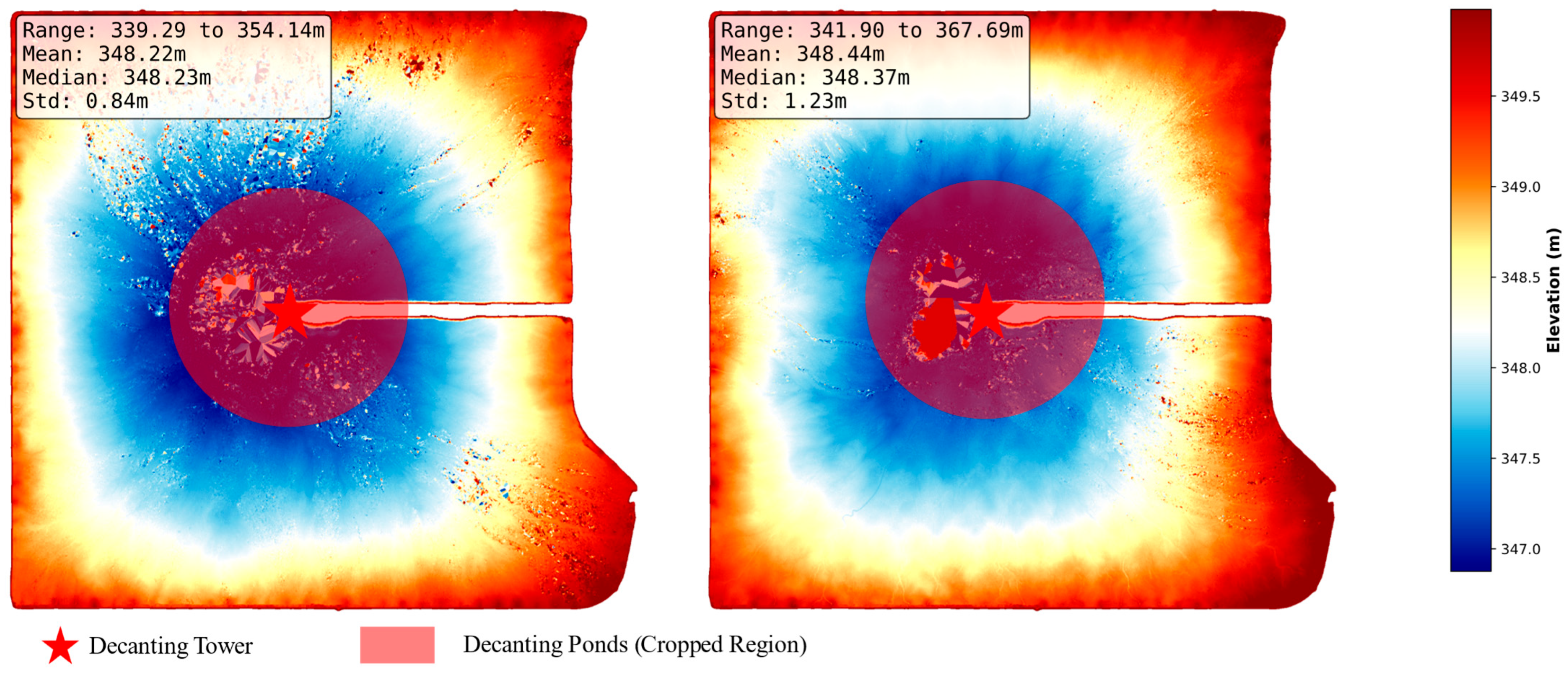
Figure 2 presents heatmaps illustrating elevations derived from the DEMs. To enhance the visualization of effective terrain data, extreme elevation values were masked by applying a 2nd to 98th percentile range. This approach excludes outliers and helps define a confidence threshold for valid pixels within the DEMs. Analysis of these heatmaps indicates that, in addition to the outer boundary regions excluded by the primary shapefile, significant outliers occurred around the decanting tower areas. This is attributable to the presence of tailing ponds, where unconsolidated, undrained tailings can cause substantial and highly variable surface elevations, leading to anomalous data points during DEM generation.
A comparative analysis of the two processed DEMs is summarized in Table 1. Both datasets utilize the same Coordinate Reference System (CRS), EPSG: 28351 (GDA94/MGA zone 51), which ensures spatial consistency vital for subsequent change detection analyses. Furthermore, both DEMs maintain an identical spatial coverage of 90.4% within the defined study area. This consistent footprint facilitates effective data processing and allows for robust comparative calculations between the epochs.
The DEM acquired on 29 January 2025 possesses a pixel resolution of 0.03750 m. This initial DEM exhibits elevations ranging from a minimum of 339.3 m to a maximum of 354.1 m, with an average and median elevation of approximately 348.2 m. Approximately one month later, the subsequent DEM acquired on 26 February 2025 features a finer resolution of 0.02634 m. The high-resolution characteristic of both datasets enables the detailed capture of fine-scale topographical features. For this later DEM, the elevation ranges from a minimum of 341.9 m to a maximum of 367.7 m. Its average elevation increased slightly by 0.2 m to 348.4 m, a value also like its median. A notable difference is observed in the standard deviation, which is higher for the later DEM (1.231 m) compared to the previous one (0.838 m). This increase in standard deviation suggests a greater variability or roughness in the terrain surface as captured in the more recent survey, potentially reflecting ongoing depositional processes and morphological changes within the TSF.

4.2. DEM of Difference

The DEM of Difference (DoD) method was employed to quantify erosion and deposition on the tailing beaches, a widely used technique in geomorphic change detection. Surface deformation between two or more DEMs, acquired at different time intervals, can be quantified through pixel-wise subtraction [43,44], as illustrated in Equation (1):
D E M = D E M t 1 D E M t 0 + ϵ ,
where t 0 represents the DEM at the initial time, t 1 is the DEM at the subsequent time, and ϵ accounts for errors and uncertainties. The DoD is computed on a pixel-by-pixel basis, generating a raster in which cell values indicate stable (zero), depositional (positive), or erosional (negative) changes on the tailings surface. Uncertainties in DoD analysis primarily arise from errors inherent in DEM generation and data acquisition. Additional noise may be introduced by local variability, weather conditions, and environmental disturbances.
To enhance the reliability of DEMs and detect subtle topographic variations, Z-score normalization (Equation (2)) was applied. This standardization of elevation values removes the influence of absolute scale and mean trends. The transformation enhances the detection of localized topographic anomalies by converting elevation values into deviations from the mean, measured in units of standard deviation:
D E M n o r m =   D E M ( x , y )   μ σ ,
where D E M ( x ,   y ) is the original elevation value of a pixel, μ   is the mean elevation of the DEM, and σ is the standard deviation. This method enhances the prominence of relative topographic features, such as deltas and rills, while concurrently reducing background noise and preserving local details.
Furthermore, to eliminate the influence of undrained tailings and enhance the robustness of DL predictions, tailing pond areas, typically located around the decanting tower, were excluded from analysis and defined as invalid regions. DoD rasters were generated from the DEM time series, resulting in single change detection maps from two DEM acquisitions. Thresholds, corresponding to the 5th and 95th percentiles were applied to filter noise and define confidence intervals for meaningful change. The resulting DoD rasters were subsequently utilized to train predictive models and to support spatial mapping and estimation of delta formation and flow channel development on tailings beaches.

4.3. Terrian Factors

The deposition and erosion patterns on tailings surface, driven by emissions through pumping systems, are significantly influenced by microtopographic features [44]. This study extracts a comprehensive set of such features from DEMs to investigate their effects on geomorphic processes. The derived features include elevation, slope, aspect, spatial location, Slope Length (LS) factor, Roughness, Topographic Position Index (TPI), Relief Index (RI), Planform Curvature (PC), Profile Curvature (PF), and General Curvature (GC). These factors were selected because they capture terrain characteristics such as slope, curvature, roughness, and relative position, which influence erosion and deposition [44,45,46,47], and they can be derived from DEMs using tools like RichDEM and GDAL.
The baseline DEM provides raw elevation data, representing altitude values for each grid cell. This elevation data is standardized prior to use. Slope, defined as the gradient of each pixel, is min-max normalized. Aspect, representing slope orientation (azimuth), is decomposed into continuous cosine and sine components (CosA, SinA) for compatibility with DL algorithms. The spatial location is defined using a coordinate system with its origin at the bottom-left corner of TSF Cell 3, where the X-axis aligns with the bottom boundary and the Y-axis aligns with the left boundary. A spatial coordinate (x, y), indicating each pixel’s geographic position within the study area, and are normalized to the range [0, 1].
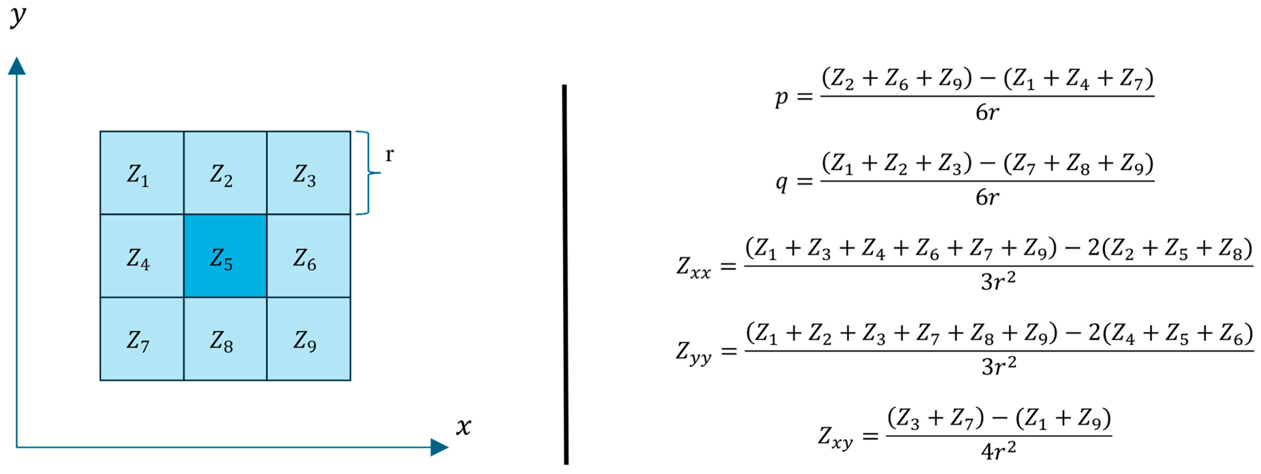
Microtopographic attributes are computed using a standardized 3 × 3 moving window approach. Each focal cell ( Z 5 ) is analyzed along with its eight neighbors ( Z 1 to Z 9 ), using r to denote cell resolution (Figure 3). The subsequent details the specific factors derived using this window-based approach.
The LS factor quantifies the horizontal distance over which water can flow and accumulate on a slope, serving as an indicator relevant to soil loss estimation. The LS equation is expressed as
L S = F A × r m ,   m = β   /   ( 1 + β ) ,
where FA represents flow accumulation, r denotes the cell resolution, and β representing the slope angle in radians. This expression is a simplified adaptation of formulations commonly used in erosion models [48]. While it does not incorporate all parameters typically included in full erosion models such as slope thresholds, flow convergence indices, it provides a computationally efficient proxy for relative slope length that is suitable for comparative analysis across the study area.
The roughness measures the variation and irregularity of elevation, or standardized surface height, for individual pixels within the analytical window. In this study, it was calculated as the mean absolute deviation of elevations, a simple and widely used descriptor of surface variability in geomorphometric analysis [49]. It is computed as
R o u g h n e s s = 1 n | Z i j z ¯ i | ,
where n is the number of pixels in the window, Z i j is the elevation of a pixel within the window, and z ¯ i is the average elevation of the pixels within that window. A higher roughness value suggests increased hydraulic resistance, which leads to reduced erosion rates.
TPI characterizes the local elevation differential between a focal cell and its surrounding neighborhood. It is expressed as
T P I = Z 5 Z ¯ ,
where Z 5 is the elevation of the central pixel within the 3 × 3 window, and Z ¯   is the average elevation of all cells within that window. This index effectively classifies relative landscape positions: positive TPI values indicate peak positions relative to the neighborhood, which are less prone to tailing accumulation, whereas negative values correspond to relative valleys, exhibiting a tendency for accumulation.
The RI quantifies the local elevation range normalized by the area of the analytical window. It is calculated as
R I = ( Z m a x Z m i n ) n r 2 ,
where Z m a x   and Z m i n represent the maximum and minimum elevation values within the 3 × 3 window, respectively. n is the number of pixels within the window, and r is the cell resolution. A greater RI value indicates more complex local topography and potentially higher gravitational potential energy.
Planform Curvature (PC) characterizes the rate of change in aspect along a contour line. Profile Curvature (PF) quantifies the rate of change in slope along the direction of maximum slope. General Curvature (GC) represents the overall curvature of the surface and is calculated as the sum of profile and planform curvatures. In this context, with p and q representing the first derivatives of elevation in the x and y directions, respectively, and Z x x , Z y y , Z x y being the second-order partial derivatives of elevation, these curvatures are formulated as
P C = Z x x p 2 + 2 Z x y p q + Z y y q 2 p 2 + q 2 3 / 2 ,
P F = Z x x q 2 2 Z x y p q + Z y y p 2 p 2 + q 2 1 / 2 ,
G C = Z x x + Z y y .
These comprehensive metrics characterize the overall morphology of the local surface. Negative values typically indicate convex surfaces, while positive values represent concave surfaces, although the specific interpretation can depend on the sign convention used in the formulas for Planform and Profile curvature.
The methodological approach uses the elevation statistics from the initial DEM as the baseline, against which the subsequent DEM (dated 26 February 2025) is compared. These two DEMs undergo an alignment process, reportedly to a 0.05 m level of precision, primarily to compute a Difference in DEMs (DoD). Concurrently, twelve distinct spatial and topological factors, inclusive of x and y coordinates, are derived from the 29 January 2025 DEM; these factors constitute the input features for subsequent DL predictions.
Further refinement of the dataset involves focusing on effective operational areas delineated by project-specific shapefiles and a tailing pond mask. Within these defined boundaries, relative topological features are extracted from the DoD patches by leveraging their spatial coordinates. This structured feature extraction culminates in a dataset organized into 13 distinct channels, with each channel comprising 208 patches. This multi-channel, patch-based dataset forms the final input for the DL model.

4.4. Dataset Partitioning and Spatial Configuration

The dataset utilized in this study consists of approximately 20,000 patches for each site, with each patch comprising 14 channels, including one DoD channel as target and 13 terrain features as input, that represent various topographic attributes and their temporal changes. To ensure a robust evaluation, the data was partitioned into training and testing sets, with 80% allocated for training and the remaining 20% for testing. A key consideration in this partitioning was the complete avoidance of spatial overlap between the two sets, thereby preventing any data leakage. Furthermore, 10% of the training data was designated as a validation set, which served the dual purpose of hyperparameter tuning and implementing early stopping criteria to prevent model overfitting.
In addition, to assess the stability and generalizability of these models across different subsets of the data, a 5-fold cross-validation was performed on the entire dataset. The consistent performance observed across all folds provides strong evidence of the models’ robustness.
For the training of the DL models, specifically the multilayer perceptron (MLP), fully convolutional network (FCN), and residual network (ResNet), a batch size of 32 was selected to optimize computational efficiency. In addition, hyperparameters were selected through empirical tuning based on validation loss. Learning rates in the range of 0.0005–0.005 and batch sizes of 16–64 were tested, with the final settings chosen as: batch size = 32, maximum epochs = 100, early stopping with patience = 10, Adam optimizer (initial learning rate = 0.001, weight decay = 1 × 10⁻⁴), and MSE loss. A learning-rate scheduler reduced the rate by a factor of 0.5 if validation loss did not improve for five epochs.
All computational experiments were conducted on Amazon Web Services (AWS) G5.8xLarge instances equipped with NVIDIA A10 GPUs (24 GB VRAM) and over 128 GB of CPU memory. Meanwhile, to enhance the capacities of the spatial context and capture spatial context while adhering to GPU memory constraints, both the computed DoD maps and the derived spatial features were segmented into patches of three distinct sizes: 64 × 64, 128 × 128, and 256 × 256 pixels. This segmentation employed a sliding window approach with a 50% overlap, ensuring comprehensive spatial coverage and contextual continuity across patch boundaries.

4.5. Deep Learning (DL) Algorithms

To explore the relationships between observed elevation changes and derived spatial features, Pearson’s correlation analysis was conducted. This analysis helps identify which spatial features are most strongly associated with elevation change patterns, providing insights into potential controlling factors. It calculates a correlation coefficient (r) to quantify the strength and direction of linear associations between variable pairs, along with a corresponding p-value to assess statistical significance.
A suite of DL algorithms, including multilayer perceptron (MLP), fully convolutional network (FCN), and residual network (ResNet), was utilized to predict elevation changes, such as delta and rill deformations, based on the extracted micro-topographical factors and geological features. The MLP was employed as a baseline to integrate DEM-derived attributes in a non-spatial manner, thereby emphasizing global correlations among features. The FCN was selected to preserve the two-dimensional structure of terrain patches, enabling the detection of localized deposition–erosion patterns. ResNet extends this approach by incorporating residual connections, which facilitate deeper training and allow for the representation of more complex, multi-scale geomorphic interactions. These architectures were selected to capture a range of spatial and structural patterns within the data. In addition, to evaluate the influence of spatial context, input image patches of three sizes ( 64   ×   64 ,   128   ×   128 ,   a n d   256   ×   256 pixels) were used. These scales reflect progressively broader terrain coverage, enabling a comparative assessment of how local versus regional features affect model performance. Each neural network architecture was adapted to accept different patch sizes while preserving its core structure. This design enables consistent multi-scale analysis, offering insights into the spatial extent over which microtopographic and geological features influence deformation dynamics.

4.5.1. Multilayer Perceptron (MLP)

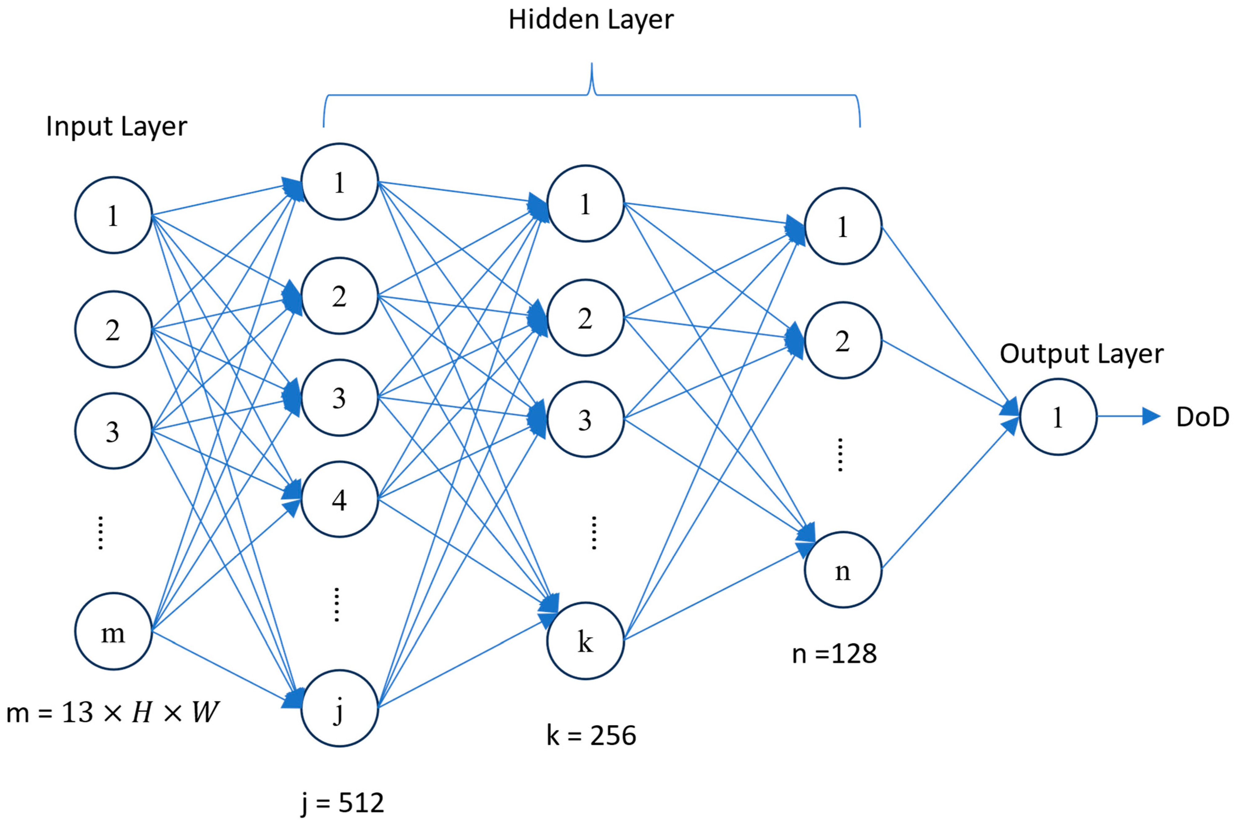
In this study, the multilayer perceptron (MLP) [50] model, a fully connected feedforward neural network, was employed to perform patch-level regression for terrain deformation prediction. The model is designed to accommodate varying input patch sizes ( 64   ×   64 ,   128   ×   128 ,   256   ×   256 ) of 13 spatial feature channels by adjusting the dimensionality of the input layer accordingly. For these patch sizes, the resulting input dimensions are 53,248, 212,992, and 851,968, respectively.
The architecture consists of three hidden layers with 512, 256, and 128 neurons, each followed by batch normalization and dropout to enhance training stability and reduce overfitting (Figure 4). The final linear layer produces a single scalar output representing the predicted average DoD (elevation change) for the entire patch. This model provides a lightweight and computationally efficient baseline, capturing nonlinear associations between micro-topographical features and observed surface changes through hierarchical representation learning.
The primary advantage of the MLP model lies in its relative simplicity and computational efficiency. Each neuron applies an activation function to the weighted sum of its inputs, enabling the model to capture complex nonlinear relationships. In predicting elevation changes, MLP can learn intricate patterns between microtopographic factors and the observed elevation responses.

4.5.2. Fully Convolutional Network (FCN)

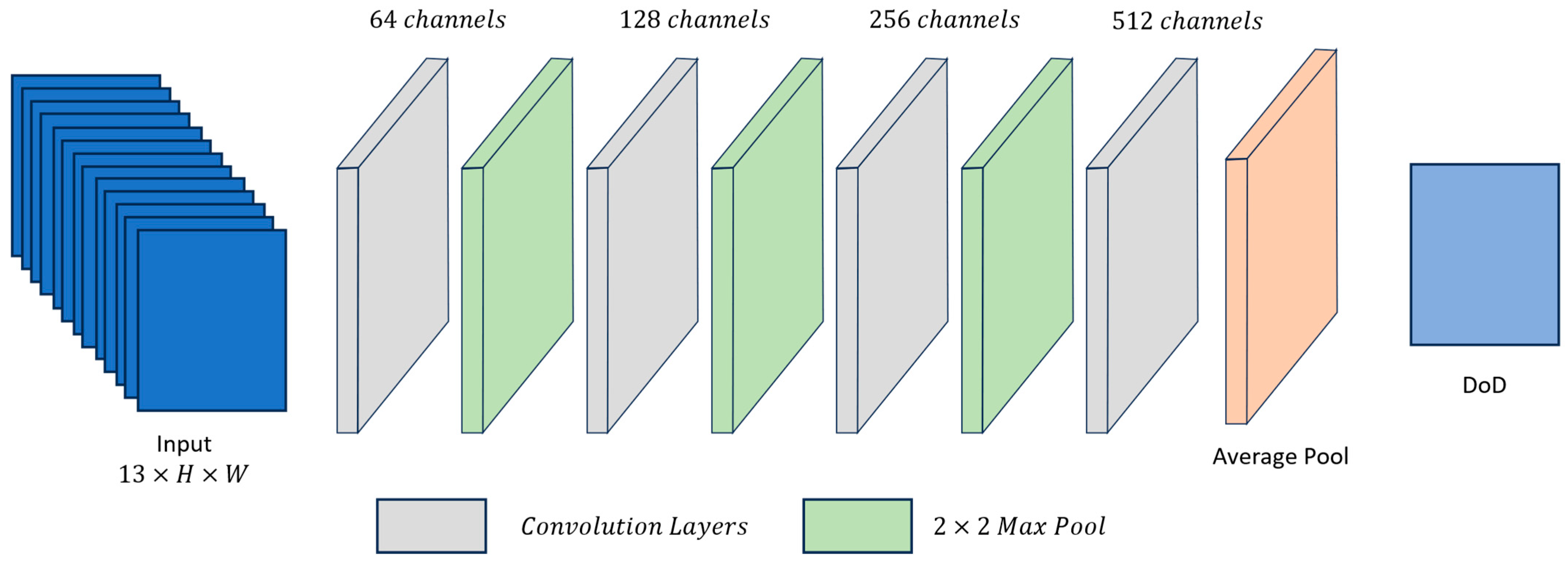
The fully convolutional network (FCN) [51] adopted in this study is a convolutional encoder architecture tailored for patch-level DoD prediction tasks. Unlike traditional fully convolutional networks, the FCN processes spatial input data using a sequence of convolutional layers that preserve the spatial structure of the input. The encoder comprises four sequential convolutional blocks, each containing two convolutional layers followed by batch normalization and ReLU activations, interleaved with max-pooling operations to progressively reduce spatial resolution and increase feature abstraction.
Across the four blocks, the feature map resolution reduces proportionally with input size ( 256 × 256   to   16 × 16 ;   128 × 128   to   8 × 8 ;   64 × 64   to   4 × 4 ), while the number of feature channels increases from 64 to 512 (Figure 5). A global average pooling layer is applied to the final feature maps, compressing the spatial information into a fixed-length 512-dimensional vector regardless of input size. This feature vector is then passed through a fully convolutional regression head to produce DoDs.
This architecture is well-suited for handling high-dimensional input data, such as detailed spatial features derived from DEMs. FCNs are powerful for capturing complex spatial interactions, which is particularly beneficial when combined with feature engineering that emphasizes critical spatial patterns.

4.5.3. Residual Network (ResNet)

A residual network (ResNet) [52] architecture was also implemented to evaluate its effectiveness in modeling terrain deformation. The model follows a standard ResNet encoder design and leverages residual blocks to facilitate deeper network training without suffering from vanishing gradients. The network begins with a 7   ×   7 convolution and max-pooling operation, followed by four stages of residual layers, each containing multiple residual blocks with identity shortcuts. These layers progressively reduce spatial resolution while increasing channel depth ( 64     128     256     512 ), allowing the model to extract hierarchical spatial features from input patches (Figure 6).
After the final residual stage, global average pooling is used to aggregate spatial features into a fixed-length 512-dimensional vector. A fully convolutional layer then maps this representation to a single scalar output representing the average DoD across the input patch. This architecture incorporates skip connections within the residual blocks, which allows the model to integrate features across multiple scales, leading to accurate and detailed predictions. In the context of elevation change prediction, ResNet can capture complex, multi-scale features from high-resolution spatial data, making it effective for modeling intricate elevation deformation patterns.

4.6. Evaluation Metrics

Model performance was evaluated using several standard regression metrics, including Mean Absolute Error (MAE), Mean Squared Error (MSE), Root Mean Squared Error (RMSE), Mean Absolute Percentage Error (MAPE), and the coefficient of determination (R2), as defined in Equations (10)–(13). Additionally, residual analysis was conducted by computing the mean and standard deviation of the prediction errors over the test patches to assess spatial error distribution:
M A E   =   1 n y i     y ^ ,
M S E = 1 n   ( y i y ^ ) 2 ,
R M S E = M S E ,
R 2 = 1 y i   y ^ 2 y i y ¯ 2 ,
where the n is the total number of pixels in the patch, y is the true elevation of the i-th pixel,   y ^ is the predicted elevation of the i-th patch, and y ¯ is the mean elevation of i-th patch. These evaluation metrics provide a comprehensive assessment of the accuracy and robustness of the models across the spatial domain of the elevation change data.

5. Results

This section presents the empirical findings of the study. First, the spatial patterns of DoD within the TSF are characterized. Next, the performance of three DL models in predicting these changes is evaluated. Finally, the best-performing model is interpreted to understand the key drivers of sediment deposition and erosion.
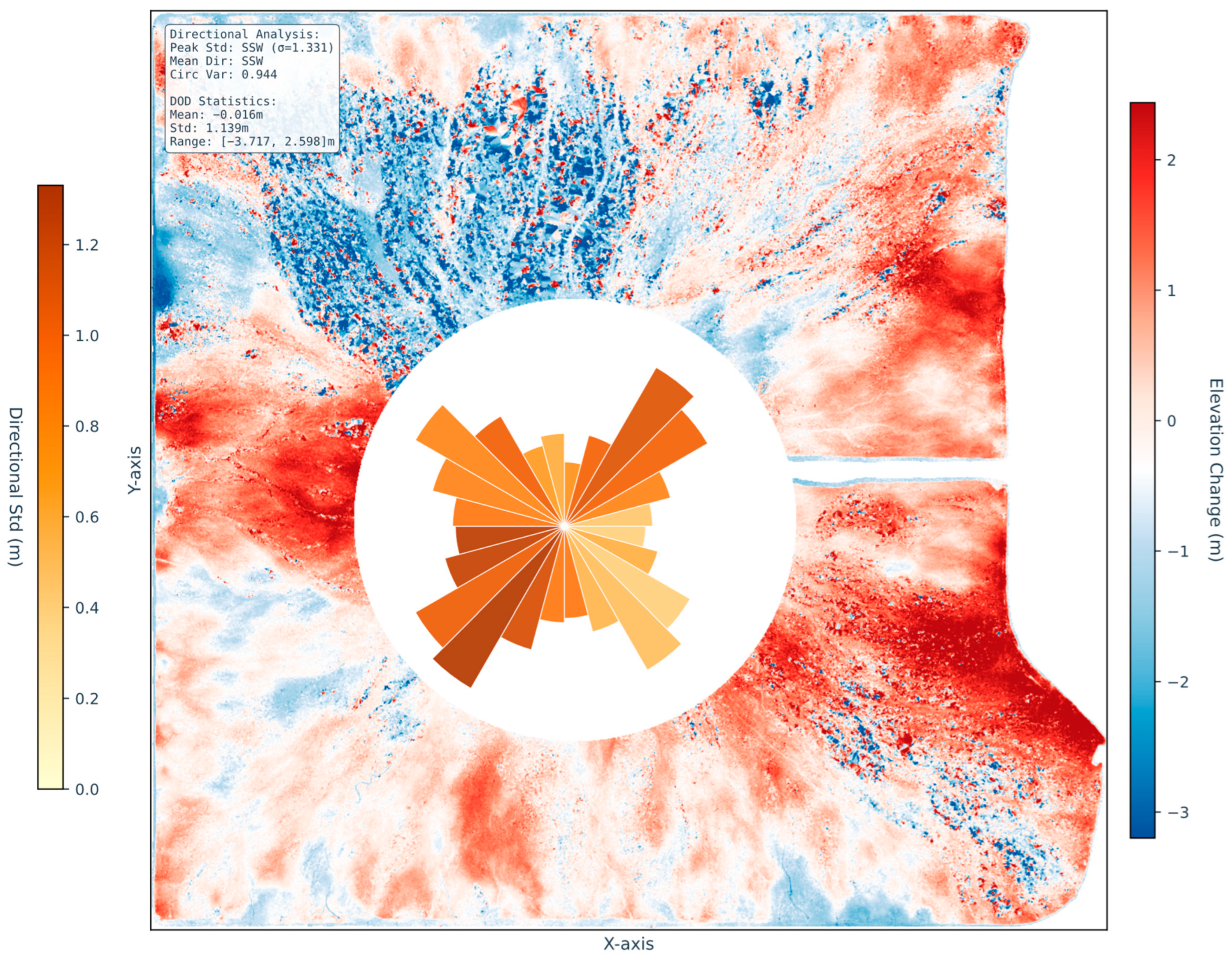
Spatial Patterns from DEM of Difference Analysis of the DoD heatmap reveals alternating zones of positive and negative elevation change across the TSF, with varying magnitudes and irregular spatial distribution (Figure 7). While the mean elevation change across the entire area is near-zero ( 0.016   m ), suggesting a state of net equilibrium, the high standard deviation ( 1.139   m ) and wide range ( 3.717   m   to + 2.598   m ) indicate significant spatial heterogeneity.
The major sediment transport pathway is evident toward the south-southwest (SSW), characterized by a large, contiguous zone of heavy deposition (dark-red areas). A rose diagram of sediment transport direction further confirms this strong, unimodal trend ( ω   =   1.306 , c i r c u l a r v a r i a n c e   =   0.944 ). In contrast, the northeastern (ENE) and northwestern (WNW) margins exhibit extensive elevation loss (blue regions), attributable to sediment compaction, erosion, or gravitational redistribution. The symmetrical distribution of deposition to the east and west suggests discharge-controlled flow patterns.
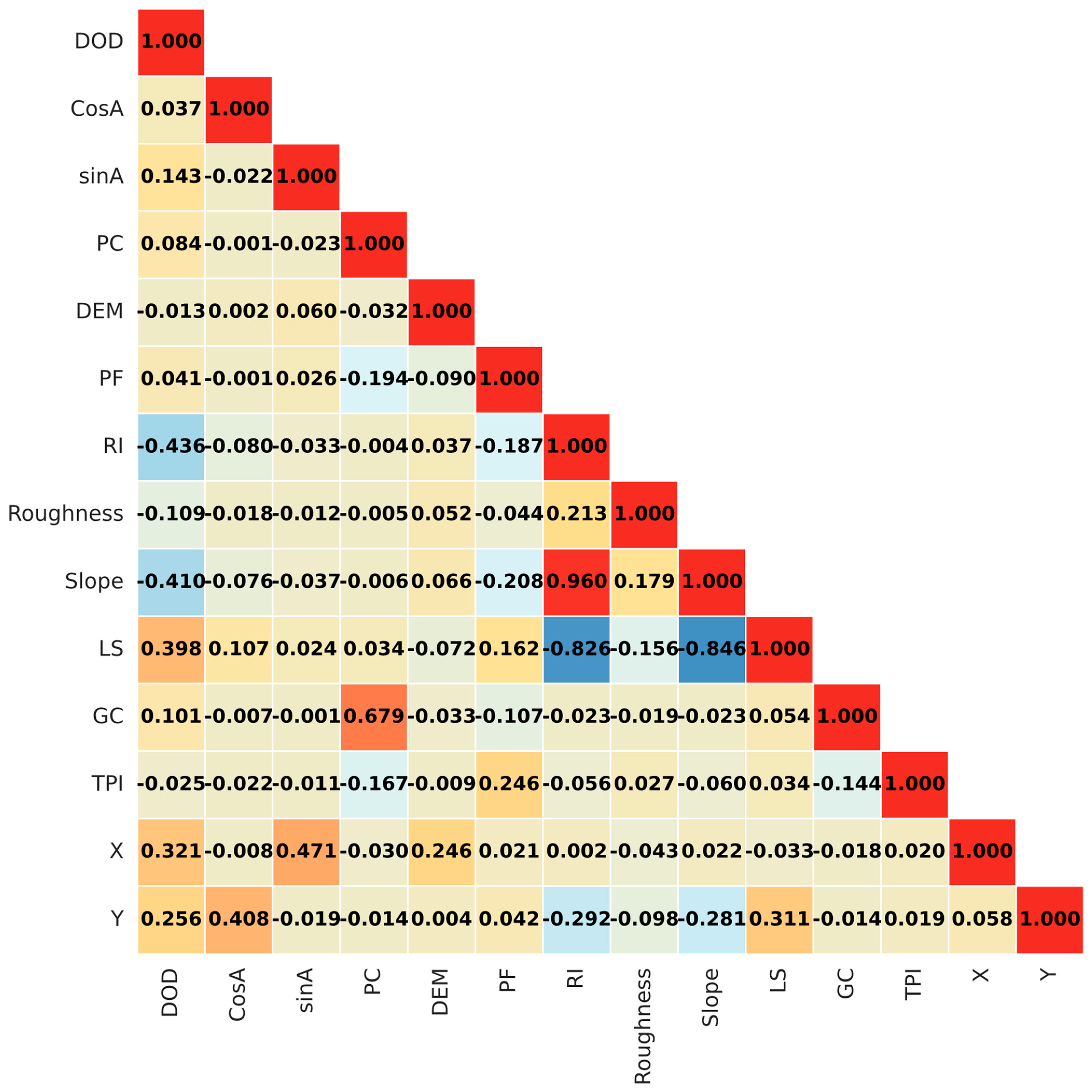
To identify the primary factors influencing these elevation changes, a Pearson correlation analysis was performed between the DoD and various terrain attributes (Figure 8). The analysis reveals that spatial coordinates ( X and Y ) have a moderate positive correlation with DoD ( r   =   0.346 and r   =   0.267 , respectively), highlighting the influence of material source proximity and flow direction. Conversely, steeper and rougher terrains are less prone to sediment deposition, as indicated by the negative correlations for slope ( r   =   0.273 ) and roughness ( r   =   0.413 ). Overall, Pearson’s relation highlights interdependencies among terrain parameters. To further evaluate how well these spatial features can predict DoD, we applied three representative learning models (MLP, FCN, and ResNet) across multiple spatial contexts.

5.1. Prediction Model

Three DL architectures (MLP, FCN, and ResNet) were evaluated for their ability to predict DoD patterns using varying spatial contexts (patch sizes of 64 × 64, 128 × 128, and 256 × 256 pixels). Model performance was assessed on a held-out test dataset, with results summarized in Table 2.
A clear trend emerged that model performance improved with increased patch size for all architectures, highlighting the importance of spatial context in predicting elevation changes. The ResNet model, particularly with a 256   ×   256 patch size, demonstrated superior performance across all evaluation metrics. It achieved the lowest MAE ( 0.0893   m ), RMSE ( 0.2304   m ), and the highest R2 ( 0.8857 ). In contrast, while FCN outperformed MLP, its best R2 value (0.8736) was still lower than ResNet. The MLP, especially at smaller patch sizes, showed signs of overfitting, performing well on training data but poorly on the test set, indicating that it lacks the capacity to capture spatial structure and is therefore less suitable for explaining deposition processes.
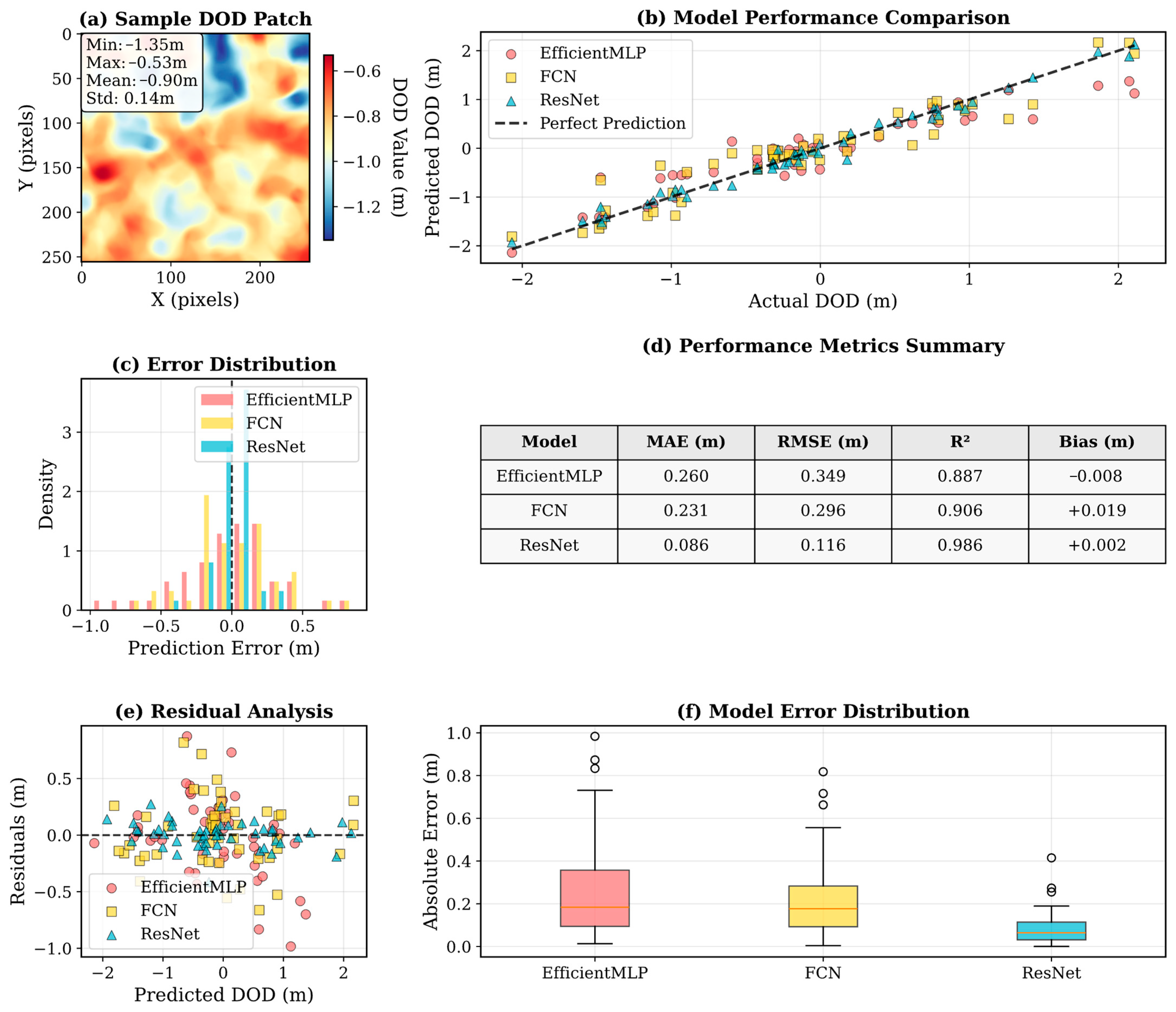
Further analysis of the 256   ×   256 models based on a DoD sample patch (Figure 9a) confirm ResNet’s superior predictive accuracy and stability (Figure 9b–f). The scatter plot of actual versus predicted DoD values (Figure 9b) shows ResNet’s predictions clustering most tightly along the perfect prediction line. The error distribution (Figure 9c) is visibly narrower and more centered on zero for ResNet compared to FCN and MLP.
The residual analysis reinforces this conclusion. ResNet exhibits the most tightly centered and homoscedastic residuals (Figure 9e), with the lowest median absolute error (Figure 9f), indicating consistent prediction accuracy across the range of DoD values. While FCN and MLP show higher variance and systematic bias, particularly a tendency to underestimate deposition, ResNet produces highly accurate and reliable predictions, making it the optimal model for subsequent spatial–temporal trend assessment.

5.2. Model Interpretability Based on SHAP

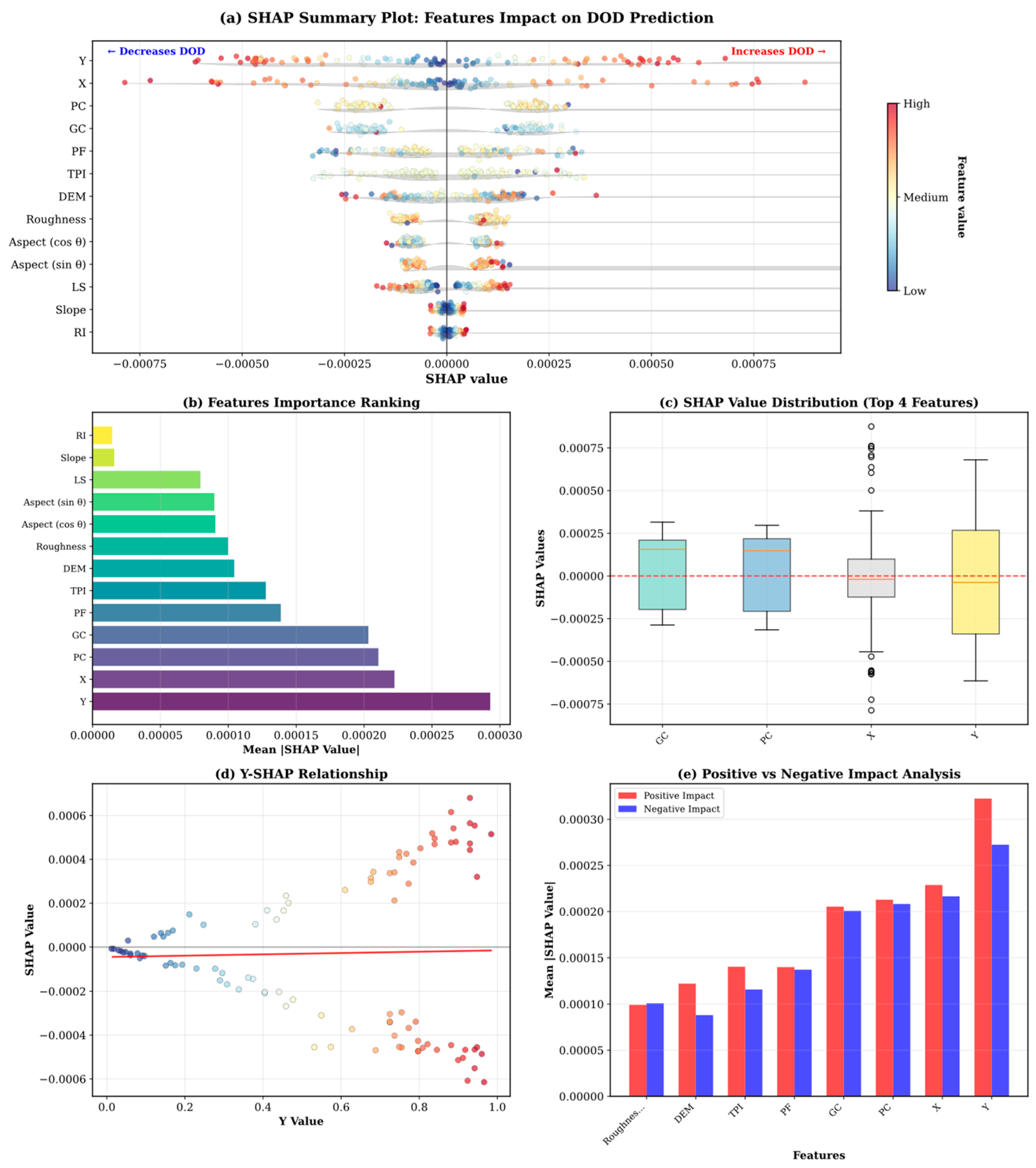
To interpret the predictive behavior of the optimal ResNet model ( 256   ×   256 input patch), SHapley Additive exPlanations (SHAP) were applied to quantify the contribution of each input feature to model output, as revealed in Figure 10. This interpretability analysis allows for a deeper understanding of the terrain attributes driving predicted surface elevation change within the TSF.
The SHAP summary plot (Figure 10a) and the ranking of mean absolute SHAP values (Figure 10b) rank input features by their average contribution to the model’s predictions. Spatial coordinates, particularly the Y and X positions, emerged as the most influential variables, reflecting the strong directional control of discharge location on sediment deposition patterns. This is consistent with experimental observations where material flow radiates outward from specific discharge points, with coarser particles settling proximally and finer particles transported farther away [53]. Among the terrain-derived attributes, slope, planform curvature, general curvature, and flow accumulation were also ranked highly. Slope exhibited a negative SHAP contribution, indicating that steeper terrain was associated with reduced predicted deposition, because of gravitational flow and limited retention on inclined surfaces. In contrast, positive SHAP values were associated with higher curvature and flow accumulation values, pointing to a tendency for sediment to accumulate in concave and convergent topographies.
In addition, SHAP value distributions (Figure 10c) reveal that many features exert nonlinear and context-dependent effects. For instance, the influence of slope varies depending on the broader spatial setting, and curvature may contribute positively or negatively depending on whether the local geometry promotes dispersion or retention. The dependency plot for the Y-coordinate (Figure 10d) shows a consistent, monotonic relationship with predicted deposition, reaffirming the importance of discharge directionality. Figure 10e further separates positive and negative SHAP contributions, showing that some features (e.g., curvature and flow accumulation) exert both positive and negative influences depending on local geomorphic context, while spatial coordinates (X, Y) consistently dominate in both directions. These results indicate that the model has learned physically meaningful interactions among input features, beyond simple linear relationships.
In conclusion, the SHAP analysis confirms that the ResNet model captures complex topographic controls on tailings behavior and supports its use as a tool for extracting interpretable insights from spatial data.

6. Discussion

6.1. Interpretation of Dominant Factors on Tailings Deposition

Similar applications of deep learning for geomorphic change detection have been reported in studies of landslide dynamics and related surface processes [43], yet applications in the context of TSFs remain rare. The findings of this study are broadly consistent with these studies in showing that slope and curvature exert primary controls on local deposition–erosion patterns. However, the explanatory power achieved here is substantially stronger: the proposed framework accounts for approximately 90% of the observed variability in deposition, compared with the much lower explanatory capacity typically reported in traditional geomorphic analyses.
The SHAP-based interpretation of the ResNet model provides valuable insights into the topographic controls on surface change in TSFs. The dominance of spatial coordinates (X and Y) in the model confirms the critical influence of discharge distance on deposition patterns. This directional dependency aligns with physical expectations, as tailings are discharged from fixed points and flow radially outward, influenced by initial momentum and local elevation gradients. Among the terrain factors, slope consistently exhibited a negative contribution to deposition, reflecting reduced sediment retention on steeper surfaces due to gravitational transport. Curvature-related features, particularly planform and general curvature, had strong positive effects when surfaces were concave, promoting local deposition. These findings are consistent with sediment transport study, where concave microtopography often acts as an accumulation zone and convex features tend to promote flow divergence [54].
By distinguishing depositional zones associated with concave curvature from erosional regions linked to steep slopes, the model demonstrates the capacity of DL to capture complex, nonlinear terrain–deposition relationships that are not explicitly encoded in conventional approaches.
Furthermore, the SHAP results show that multiple features interact nonlinearly, reinforcing the notion that tailings deposition is governed by a combination of discharge direction, topographic form, and localized flow behavior, rather than any single controlling variable.

6.2. Significance of DL for Predictive Geomorphic Modeling

This study highlights the effectiveness of DL, particularly convolutional neural network architectures, for predicting surface changes in TSFs. The superior performance of the ResNet model, especially when trained on large spatial patches (256 × 256), demonstrates the importance of contextual information in modeling surface deformation. This result suggests that both local microtopography and broader spatial gradients jointly influence tailings behavior, and DL architecture can integrate these patterns effectively.
Unlike traditional process-based models, which require predefined assumptions and complex parameter calibration, DL offers a flexible, data-driven approach that can extract hidden relationships directly from high-resolution observational data. The integration of SHAP into the analysis provides a critical interpretability layer, allowing researchers and engineers to understand which input variables drive predictions and how they interact. This overcomes a key limitation often associated with black-box ML models, increasing trust and transparency.
Additionally, the patch-level prediction strategy, enabled by average pooling layers in the network, provides a robust summary of localized terrain dynamics. Instead of predicting individual pixel values, which may be noisy or affected by data artifacts, the model learns to estimate the average elevation change across a spatially coherent region. This enhances stability, reflects real-world operational scales, and aligns better with practical applications such as discharge zone monitoring or surface grading decisions.

6.3. Practical Implications for TSF Management

The results of this study offer several actionable insights for improving TSF management through data-driven surface change prediction. By accurately predicting DoD using DL models informed by terrain features, the framework enables early identification of areas prone to excessive deposition or erosion. This supports proactive intervention to maintain slope stability, optimize discharge strategies, and prevent unintended flow paths.
The strong spatial dependency captured by the model, particularly the influence of spatial distributions and slope, can guide strategic discharge planning by identifying zones of effective sediment distribution. Additionally, features like flow accumulation and curvature, which reflect the hydrodynamic behavior of facilities, can be used to determine potential deposition deltas or water-retention zones, enabling more effective dewatering management and drainage control.
From an operational perspective, the model’s interpretability enhances trust and usability for engineers, making it more feasible to integrate into routine TSF monitoring workflows. With adequate retraining, the framework can be extended to other TSFs, contributing to standardized, site-specific surface change forecasting.
Ultimately, this approach bridges the gap between black-box prediction and process-aware decision-making, offering a practical tool to support safe, efficient, and adaptive tailings management.

6.4. Limitations and Future Direction

Although this study demonstrates the potential of deep learning for interpreting tailings deposition, several limitations must be acknowledged. Despite the use of UAV photogrammetry, high-resolution cameras, and DEM construction techniques that provide fine-scale surface detection, uncertainties persist due to the inherent complexity of sedimentation processes and the constraints of grid-based representations. Survey hardware, software, processing workflows, study area extent, monitoring frequency, and logistical considerations may all introduce additional errors, which limit the confidence with which surface changes can be quantified. These challenges were compounded by restrictions on site access due to confidentiality agreements and field detection rights, which prevented more detailed ground validation and testing. Incorporating sensitivity and uncertainty analysis in future work would strengthen the robustness of the framework and enhance its relevance for risk assessment.
The framework was trained on data from a single TSF, and its learned parameters are therefore specific to the material properties, climatic conditions, and operational practices of that site. Because additional in situ investigations were not permitted, broader validation was not feasible. Future research should therefore apply the framework to multiple TSFs with different ore types and operational contexts to assess its generalizability.
Finally, the current model is static, predicting deposition outcomes for individual survey intervals rather than continuous temporal evolution. A critical avenue for future work is the development of dynamic models that integrate time-series topographic surveys and operational data, enabling forecasts of landform change over extended periods and providing valuable insights for long-term TSF monitoring and closure planning.

7. Conclusions

This study showed that DL combined with SHAP, can identify the main terrain features that control tailings deposition using UAV-derived DEMs. Of the three tested models, ResNet with larger input patches gave the best results, showing that both local microtopography and wider spatial context are important. SHAP analysis confirmed that spatial coordinates (linked to discharge distance), together with curvature and slope, were the strongest drivers of deposition, supporting the physical meaning of the outputs.
The novelty of this work is the first systematic use of DL and SHAP on field TSF data, giving more explanatory power than traditional geomorphic methods. Still, there are limits. The results are affected by uncertainty in UAV data, training on only one site, and the static design of the model, which does not include dynamic hydrological processes.
This study demonstrates that DL models, when trained on real-world terrain data, can effectively capture complex and spatially variable sediment dynamics without relying on extensive physical parameterization. Moreover, the model’s interpretability enhances its utility for TSF practitioners, offering a transparent tool to support discharge management, early warning systems, and spatial planning. Future work should test the framework on more TSFs, extend it to dynamic models that can track changes over time, and add sensitivity and uncertainty analysis. These steps will improve the robustness of the approach and its value for long-term TSF monitoring and closure planning.

Author Contributions

W.L.: Writing—review and editing. Writing—original draft methodology conceptualization. R.S.F.: Supervision, writing-review and editing, conceptualization. H.X.: Supervision, writing-review and editing, conceptualization. P.S.: writing-review and editing, conceptualization. All authors have read and agreed to the published version of the manuscript.

Funding

This research received no external funding.

Data Availability Statement

Restrictions apply to the availability of these data. Data were obtained from Evolution Mining Ltd. and are available from Dr Roohollah Shirani Faradonbeh with the permission of Evolution Mining.

Acknowledgments

The authors gratefully acknowledge Curtin University for access to RONIN platforms for computation and Evolution Mining Ltd., especially Moe Moridi and Anthony Kerr, for providing DEM statistics used in this study.

Conflicts of Interest

The authors declare no conflicts of interest.

References

  1. CSP2. TSF Failures from 1915. Available online: http://www.csp2.org/tsf-failures-from-1915 (accessed on 5 June 2025).
  2. ICOLD. World Register of Dams. Available online: https://www.icold-cigb.org/ (accessed on 5 June 2025).
  3. Chambers, D.M.; Higman, B. Long Term Risks of Tailings Dam Failure; Center for Science in Public Participation: Bozeman, MT, USA, 2011; pp. 1–21. [Google Scholar]
  4. Chambers, D.M. The Increasing Number of Tailings Facility Failures: Navigating the Decade 2020–2029; Canadian Dam Association Annual Congress: Ottawa, ON, USA, 2019. [Google Scholar]
  5. Rotta, L.H.S.; Alcântara, E.; Park, E.; Negri, R.G.; Lin, Y.N.; Bernardo, N.; Mendes, T.S.G.; Souza Filho, C.R. The 2019 Brumadinho tailings dam collapse: Possible cause and impacts of the worst human and environmental disaster in Brazil. Int. J. Appl. Earth Obs. Geoinf. 2020, 90, 102119. [Google Scholar] [CrossRef]
  6. Bussular, C.Z.; Burtet, C.G.; Antonello, C.S. The actor-network theory as a method in the analysis of Samarco disaster in Brazil. Qual. Res. Organ. Manag. Int. J. 2020, 15, 176–191. [Google Scholar] [CrossRef]
  7. Department of Industry, Science and Resources, Australia. Tailings Management Handbooks. Available online: https://www.industry.gov.au/publications/leading-practice-handbooks-sustainable-mining/tailings-management (accessed on 5 June 2025).
  8. International Council on Mining and Metals (ICMM); United Nations Environment Programme (UNEP); Principles for Responsible Investment (PRI). Global Industry Standard on Tailings Management. Available online: https://globaltailingsreview.org/ (accessed on 5 June 2025).
  9. Mining Association of Canada. A Guide to the Management of Tailings Facilities, Third Edition. Available online: https://mining.ca/resources/guides-manuals/a-guide-to-the-management-of-tailings-facilities-third-edition/ (accessed on 5 June 2025).
  10. Obermeyer, J.; Alexieva, T. Design, Construction and Operation of a Large Centerline Tailing Storage Facility with High Rate of Rise. 2011. Available online: https://open.library.ubc.ca/soa/cIRcle/collections/59368/items/1.0107726 (accessed on 29 August 2025).
  11. Simms, P.; Williams, M.P.A.; Fitton, T.G.; McPhail, G. Beaching angles and evolution of stack geomoetry for thickened tailings—A review. In Paste 2011: 14th International Seminar on Paste and Thickened Tailings; Australian Centre for Geomechanics: Perth, Australia, 2011; pp. 323–338. [Google Scholar]
  12. Fitton, T.G.; Chryss, A.G.; Bhattacharya, S.N. Tailings beach slope prediction: A new rheological method. Int. J. Min. Reclam. Environ. 2006, 20, 181–202. [Google Scholar] [CrossRef]
  13. Li, A.L. Prediction of tailings beach slopes and tailings flow profiles. In Paste 2011: Proceedings of the 14th International Seminar on Paste and Thickened Tailings; Jewell, R., Fourie, A.B., Eds.; Australian Centre for Geomechanics: Perth, Australia, 2011; pp. 307–322. [Google Scholar] [CrossRef]
  14. Adamo, N.; Al-Ansari, N.; Sissakian, V.; Laue, J.; Knutsson, S. Dam Safety: Monitoring of Tailings Dams and Safety Reviews. J. Earth Sci. Geotech. Eng. 2021, 11, 249–289. [Google Scholar] [CrossRef]
  15. Adiansyah, J.S.; Rosano, M.; Vink, S.; Keir, G. A framework for a sustainable approach to mine tailings management: Disposal strategies. J. Clean. Prod. 2015, 108, 1050–1062. [Google Scholar] [CrossRef]
  16. Le Borgne, V.; Siamaki, A.; Dulmage, A. Review of Modern Recommendations for Monitoring of Tailings Storage Facilities. In Proceedings of the Tailings and Mine Waste Conference, Denver, CO, USA, 6–9 November 2022; pp. 578–587. [Google Scholar]
  17. Nan, X.; Liu, X.; Wu, B.; Zhang, H.; Song, K.; Wang, X. Coupled CFD-DEM simulation and experimental study of particle distribution and accumulation during tailings seepage process. J. Clean. Prod. 2023, 427, 139229. [Google Scholar] [CrossRef]
  18. Gao, J.; Fourie, A. Studies on thickened tailings deposition in flume tests using the computational fluid dynamics (CFD) method. Can. Geotech. J. 2018, 56, 249–262. [Google Scholar] [CrossRef]
  19. Islam, S.; Williams, D.J.; Llano-Serna, M.; Zhang, C.M. Settling, consolidation and shear strength behaviour of coal tailings slurry. Int. J. Min. Sci. Technol. 2020, 30, 849–857. [Google Scholar] [CrossRef]
  20. Tian, S.; He, Y.; Bai, R.; Chen, J.; Wang, G. Experimental study on consolidation and strength properties of tailings with different particle size distribution characteristics. Nat. Hazards 2022, 114, 3683–3699. [Google Scholar] [CrossRef]
  21. Jewell, R.J. Putting beach slope prediction into perspective. In Paste 2012: Proceedings of the 15th International Seminar on Paste and Thickened Tailings; Jewell, A.B.F.R., Paterson, A., Eds.; Australian Centre for Geomechanics: Perth, Australia, 2012; pp. 85–92. [Google Scholar] [CrossRef]
  22. Pirouz, B.; Williams, M. Prediction of non-segregating thickened tailings beach slopes–a new method. In Proceedings Tenth International Seminar on Paste and Thickened Tailings (Paste07); Fourie, A.B., Jewell, R.J., Eds.; Australian Centre for Geomechanics: Perth, Australia, 2007; pp. 13–15. [Google Scholar]
  23. Fortuna, J.; Waterhouse, J.; Chapman, P.; Gowan, M. Applying Practical Hydrogeology to Tailings Storage Facility Design and Management. Mine Water Environ. 2021, 40, 50–62. [Google Scholar] [CrossRef]
  24. Schneiderman, E.M.; Steenhuis, T.S.; Thongs, D.J.; Easton, Z.M.; Zion, M.S.; Neal, A.L.; Mendoza, G.F.; Todd Walter, M. Incorporating variable source area hydrology into a curve-number-based watershed model. Hydrol. Process. 2007, 21, 3420–3430. [Google Scholar] [CrossRef]
  25. Balaniuk, R.; Isupova, O.; Reece, S. Mining and Tailings Dam Detection in Satellite Imagery Using Deep Learning. Sensors 2020, 20, 6936. [Google Scholar] [CrossRef]
  26. Bayaraa, M.; Sheil, B.; Rossi, C. Comparison of Insar and Numerical Modelling for Tailings Dam Monitoring the Cadia Failure, Australia. In Proceedings of the IGARSS 2022–2022 IEEE International Geoscience and Remote Sensing Symposium, Kuala Lumpur, Malaysia, 17–22 July 2022; pp. 4–7. [Google Scholar]
  27. Cacciuttolo, C.; Cano, D. Spatial and Temporal Study of Supernatant Process Water Pond in Tailings Storage Facilities: Use of Remote Sensing Techniques for Preventing Mine Tailings Dam Failures. Sustainability 2023, 15, 4984. [Google Scholar] [CrossRef]
  28. Du, Z.; Ge, L.; Ng, A.H.-M.; Zhu, Q.; Horgan, F.G.; Zhang, Q. Risk assessment for tailings dams in Brumadinho of Brazil using InSAR time series approach. Sci. Total Environ. 2020, 717, 137125. [Google Scholar] [CrossRef]
  29. Thomas, A.; Edwards, S.J.; Engels, J.; McCormack, H.; Hopkins, V.; Holley, R. Earth observation data and satellite InSAR for the remote monitoring of tailings storage facilities: A case study of Cadia Mine, Australia. In Paste 2019: Proceedings of the 22nd International Conference on Paste, Thickened and Filtered Tailings; Paterson, A.J.C., Fourie, A.B., Reid, D., Eds.; Australian Centre for Geomechanics: Cape Town, South Africa, 2019; pp. 183–195. [Google Scholar] [CrossRef]
  30. NASA. Landsat Science and Data Access. Available online: https://landsat.gsfc.nasa.gov/ (accessed on 5 June 2025).
  31. Rana, N.M.; Delaney, K.B.; Evans, S.G.; Deane, E.; Small, A.; Adria, D.A.M.; McDougall, S.; Ghahramani, N.; Take, W.A. Application of Sentinel-1 InSAR to monitor tailings dams and predict geotechnical instability: Practical considerations based on case study insights. Bull. Eng. Geol. Environ. 2024, 83, 204. [Google Scholar] [CrossRef]
  32. Santosa, P.B. Evaluation of Satellite Image Correction Methods Caused by Differential Terrain Illumination. Forum Geogr. 2016, 30, 1. [Google Scholar] [CrossRef]
  33. Thangaswamy, S.S.; Kadarkarai, R.; Thangaswamy, S.R.R. Developing an efficient technique for satellite image denoising and resolution enhancement for improving classification accuracy. J. Electron. Imaging 2013, 22, 013013. [Google Scholar] [CrossRef]
  34. Rauhala, A.; Tuomela, A.; Davids, C.; Rossi, P.M. UAV Remote Sensing Surveillance of a Mine Tailings Impoundment in Sub-Arctic Conditions. Remote Sens. 2017, 9, 1318. [Google Scholar] [CrossRef]
  35. Wang, K.; Yang, P.; Hudson-Edwards, K.A.; Lyu, W.S.; Yang, C.; Jing, X.F. Integration of DSM and SPH to Model Tailings Dam Failure Run-Out Slurry Routing Across 3D Real Terrain. Water 2018, 10, 1087. [Google Scholar] [CrossRef]
  36. Gomez, J.A.; Kamran-Pishhesari, A.; Sattarvand, J. Automated Rill Erosion Detection in Tailing Dams Using UAV Imagery and Machine Learning. Arab. J. Sci. Eng. 2025, 50, 6711–6726. [Google Scholar] [CrossRef]
  37. Wang, K.; Zhang, Z.; Yang, X.; Wang, D.; Zhu, L.; Yuan, S. Enhanced Tailings Dam Beach Line Indicator Observation and Stability Numerical Analysis: An Approach Integrating UAV Photogrammetry and CNNs. Remote Sens. 2024, 16, 3264. [Google Scholar] [CrossRef]
  38. Niculiță, M.; Mărgărint, M.C.; Tarolli, P. Chapter 10—Using UAV and LiDAR data for gully geomorphic changes monitoring. Dev. Earth Surf. Process. 2020, 23, 271–315. [Google Scholar] [CrossRef]
  39. Xiang, J.; Chen, J.; Sofia, G.; Tian, Y.; Tarolli, P. Open-pit mine geomorphic changes analysis using multi-temporal UAV survey. Environ. Earth Sci. 2018, 77, 220. [Google Scholar] [CrossRef]
  40. Department of Mines Industry Regulation and Safety. Mining Proposal: Mungari TSF expansion: Cells 3 and 4 [Report Prepared by Talis Consultants]. Available online: https://minedex.dmirs.wa.gov.au/Web/sites/details/6f6f5c6b-099a-4801-a985-615940373990 (accessed on 5 June 2025).
  41. Boix-Fayos, C.; Martínez-Mena, M.; Arnau-Rosalén, E.; Calvo-Cases, A.; Castillo, V.; Albaladejo, J. Measuring soil erosion by field plots: Understanding the sources of variation. Earth-Sci. Rev. 2006, 78, 267–285. [Google Scholar] [CrossRef]
  42. Wheaton, J.M.; Brasington, J.; Darby, S.E.; Sear, D.A. Accounting for uncertainty in DEMs from repeat topographic surveys: Improved sediment budgets. Earth Surf. Process. Landf. 2010, 35, 136–156. [Google Scholar] [CrossRef]
  43. Li, Y.; Lu, X.; Washington-Allen, R.A.; Li, Y. Microtopographic Controls on Erosion and Deposition of a Rilled Hillslope in Eastern Tennessee, USA. Remote Sens. 2022, 14, 1315. [Google Scholar] [CrossRef]
  44. Abrahams, A.D.; Parsons, A.J. Resistance to Overland Flow on Desert Pavement and Its Implications for Sediment Transport Modeling. Water Resour. Res. 1991, 27, 1827–1836. [Google Scholar] [CrossRef]
  45. Darboux, F.; Huang, C.-H. Does Soil Surface Roughness Increase or Decrease Water and Particle Transfers? Soil Sci. Soc. Am. J. 2005, 69, 748–756. [Google Scholar] [CrossRef]
  46. Tarboton, D.G.; Bras, R.L.; Rodriguez-Iturbe, I. On the extraction of channel networks from digital elevation data. Hydrol. Process. 1991, 5, 81–100. [Google Scholar] [CrossRef]
  47. Shen, H.; Zheng, F.; Wen, L.; Lu, J.; Jiang, Y. An experimental study of rill erosion and morphology. Geomorphology 2015, 231, 193–201. [Google Scholar] [CrossRef]
  48. Panagos, P.; Borrelli, P.; Meusburger, K. A New European Slope Length and Steepness Factor (LS-Factor) for Modeling Soil Erosion by Water. Geosciences 2015, 5, 117–126. [Google Scholar] [CrossRef]
  49. Grohmann, C.H.; Smith, M.J.; Riccomini, C. Multiscale Analysis of Topographic Surface Roughness in the Midland Valley, Scotland. IEEE Trans. Geosci. Remote Sens. 2011, 49, 1200–1213. [Google Scholar] [CrossRef]
  50. Rosenblatt, F. Principles of Neurodynamics: Perceptrons and the Theory of Brain Mechanisms; Spartan Books: Washington, DC, USA, 1962; Volume 55. [Google Scholar]
  51. Zahnle, K.J. Photochemistry of methane and the formation of hydrocyanic acid (HCN) in the Earth’s early atmosphere. J. Geophys. Res. 1986, 91, 2819–2834. [Google Scholar] [CrossRef]
  52. He, K.; Zhang, X.; Ren, S.; Sun, J. Deep residual learning for image recognition. In Proceedings of the IEEE Conference on Computer Vision and Pattern Recognition, Las Vegas, NV, USA, 27–30 June 2016; pp. 770–778. [Google Scholar]
  53. Li, Y.; van Zyl, D. Analysing the segregation of coarse tailings particles with a zone-formation differential settling model. In Paste 2024: Proceedings of the 26th International Conference on Paste, Thickened and Filtered Tailings; Fourie, A.B., Reid, D., Eds.; Australian Centre for Geomechanics: Perth, Australia, 2024; pp. 271–282. [Google Scholar] [CrossRef]
  54. Sabzevari, T.; Talebi, A. Effect of hillslope topography on soil erosion and sediment yield using USLE model. Acta Geophys. 2019, 67, 1587–1597. [Google Scholar] [CrossRef]
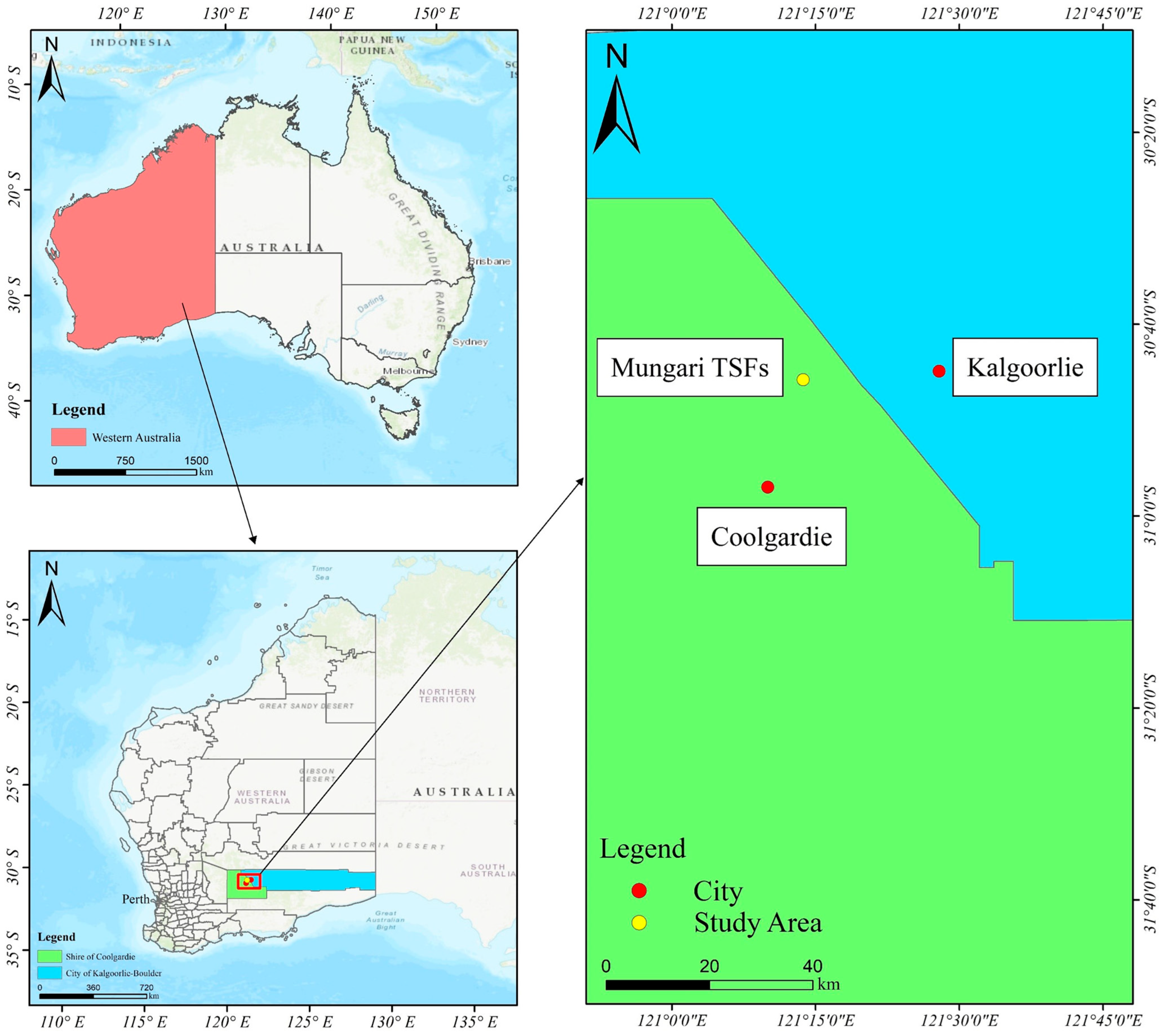
Figure 1. Location of the Mungari tailings storage facilities (TSFs) in the Kalgoorlie–Boulder region of Western Australia.
Applsci 15 10982 g001
Figure 2. Heatmaps of two months of tailings depositions. These heatmaps illustrate elevations derived from the DEMs on 29 January 2025 (left) and 26 February 2025 (right), showcasing the spatial distribution of elevation across the TSF.
Applsci 15 10982 g002
Figure 3. Schematic of the 3 × 3 moving window is used for topographic feature extraction. The central cell z 5 is surrounded by its eight neighbors z 1 z 9 , from which slope components p , q , and second-order derivatives Z x x , Z y y and Z x y are computed. The variable r denotes the spatial resolution of each grid cell. This configuration underlies the derivation of curvature and roughness metrics from the DEM.
Applsci 15 10982 g003
Figure 4. Multi-Layer Perceptron (MLP) architecture for patch-level terrain change prediction. The input layer receives j   =   13     ×     H   ×   W flattened features where H × W ∈ { 64   ×   64 ,   128   ×   128 ,   256   ×   256 } pixels, corresponding to 53,248, 212,992, and 851,968 input features, respectively. Three fully connected hidden layers with 512, 256, and 128 neurons incorporate batch normalization, ReLU activation, and dropout regularization. The output layer produces a single DoD prediction value per patch.
Applsci 15 10982 g004
Figure 5. Fully convolutional network (FCN) architecture for patch-level terrain change prediction. The encoder processes input patches with 13 feature channels and variable spatial dimensions H × W ∈ { 64   ×   64 ,   128   ×   128 ,   256   ×   256 } through four convolutional blocks. Each block performs convolution, batch normalization, ReLU activation, and max pooling, progressively extracting multi-scale features while reducing spatial dimensions. Global average pooling converts the final feature maps to a fixed-size representation, followed by regression to predict a single DoD value per patch.
Applsci 15 10982 g005
Figure 6. ResNet architecture adapted for patch-level terrain change regression. The network processes input patches (H × W × 13 where H × W ∈ { 64   ×   64 ,     128   ×   128 ,     256   ×   256 } ) through initial convolution and max pooling, followed by four residual layers with progressively increasing channels ( 64 128 256 512 ) . Adaptive average pooling ensures consistent feature representation regardless of input size, followed by a single fully convolutional layer for DoD regression output.
Applsci 15 10982 g006
Figure 7. Spatial distribution of DoD. The heatmap illustrates depositional (red) and erosional (blue) zones, while the embedded rose diagram confirms the dominant south-southwest direction of sediment transport.
Applsci 15 10982 g007
Figure 8. Heatmap of Pearson’s correlations between topographic attributes and the DoD. The matrix reveals moderate linear correlations, particularly with spatial coordinates (X, Y), slope, and roughness.
Applsci 15 10982 g008
Figure 9. Illustrative performance evaluation of the 256   ×   256 models on a representative sample patch. (a) Input DoD patch. (b) Scatter plot of predicted vs. actual DoD values. (c) Histogram of prediction errors. (d) Summary table of performance metrics for this patch (values differ from Table 2, which reports overall test-set results). (e) Residual plot of error distribution vs. predicted values. (f) Box plot of absolute model error.
Applsci 15 10982 g009
Figure 10. Model interpretability analysis using SHAP for the ResNet-256 model. (a) SHAP summary plot showing the impact of feature values on model output. (b) Mean absolute SHAP values, ranking overall feature importance. (c) SHAP value distributions for the top four features. (d) Dependency plot illustrating the relationship between the Y-coordinate and its SHAP value. (e) Analysis of features exerting both positive and negative impacts.
Applsci 15 10982 g010
Table 1. Summary of DEM information.
FeatureDEM 1 (29 January 2025)DEM 2 (26 February 2025)
Coordinate Reference System (CRS)EPSG: 28351EPSG: 28351
Effective Pixels90.41%90.41%
Pixel Resolution (m)0.037500.02634
Maximum Elevation (m)354.1367.7
Minimum Elevation (m)339.3341.9
Average Elevation (m)348.2348.4
Median Elevation (m)348.2348.4
Standard Deviation (Std)0.8381.231
Table 2. Summary of DEM information.
ModelPatch SizeTraining PerformanceTesting PerformanceResidual Analysis
MSEMAERMSE R 2 MSEMAERMSE R 2 MeanStd
MLP64 × 640.18120.33070.42570.83350.53790.55230.73340.50560.01690.7332
128 × 1280.51440.55720.71720.44020.50660.54510.71170.44870.10400.7040
256 × 2560.15720.30460.39650.79890.31320.43390.55960.5994−0.01200.5594
FCN64 × 640.20870.35370.45690.80820.17690.32240.42060.8374−0.01400.4203
128 × 1280.40210.49270.63410.56230.29050.42520.53900.6838−0.08410.5324
256 × 2560.13060.28480.36140.83290.09880.24910.31430.87360.00040.3142
ResNet64 × 640.07490.20970.27370.93120.34240.43430.58520.6853−0.01210.5850
128 × 1280.24730.38700.49730.73090.32090.43260.56640.6508−0.03830.5651
256 × 2560.01610.09870.12680.97940.0893 *0.2304 *0.2988 *0.8857 *4.56e-30.2988
Note: * indicates the best performance among models.
Disclaimer/Publisher’s Note: The statements, opinions and data contained in all publications are solely those of the individual author(s) and contributor(s) and not of MDPI and/or the editor(s). MDPI and/or the editor(s) disclaim responsibility for any injury to people or property resulting from any ideas, methods, instructions or products referred to in the content.