Article

Application of Convolutional and Recurrent Neural Networks in Classifying Plant Responses to Abiotic Stress

1
Department of Electrical and Computer Engineering, Southern University and A&M College, Baton Rouge, LA 70807, USA
2
Department of Urban Forestry, Southern University and A&M College, Baton Rouge, LA 70807, USA
3
Department of Chemistry, Southern University and A&M College, Baton Rouge, LA 70807, USA
*
Author to whom correspondence should be addressed.
Appl. Sci. 2025, 15(20), 10960; https://doi.org/10.3390/app152010960 (registering DOI)
Submission received: 7 September 2025 / Revised: 9 October 2025 / Accepted: 10 October 2025 / Published: 12 October 2025

Abstract

Agriculture is a major economic industry that sustains life. Moreover, plant health is a crucial aspect of a highly functional agricultural system. Because stress agents can damage crops and plants, it is important to understand what effect these agents can have and be able to detect this negative impact early in the process. Machine learning technology can help to prevent these undesirable consequences. This research investigates machine learning applications for plant health analysis and classification. Specifically, Residual Networks (ResNet) and Long Short-Term Memory (LSTM) models are utilized to detect and classify plants response to abiotic external stressors. Two types of plants, azalea (shrub) and Chinese tallow (tree), were used in this research study and different concentrations of sodium chloride (NaCL) and acetic acid were used to treat the plants. Data from cameras and soil sensors were analyzed by the machine learning algorithms. The ResNet34 and LSTM models achieved accuracies of 96% and 97.8%, respectively, in classifying plants with good, medium, or bad health status on test data sets. These results demonstrate that machine learning algorithms can be used to accurately detect plant health status as well as healthy and unhealthy plant conditions and thus potentially prevent negative long-term effects in agriculture.

1. Introduction

Agriculture is a fundamental industry in society that has a very important task or role in sustaining life. However, the population growth rate is outpacing the production rate of major crops, emphasizing the need for more efficient farming [1]. Agriculture is a very diverse field that includes cultivating crops, producing livestock, and managing forestry as well as engineering byproducts from these resources. In particular, plants and crops are the foundation of this vital industry [2]. These resources not only produce fruits, vegetables, and grains but they contribute to healthy ecosystems. Plants and shrubs improve soil fertility and provide food for various wildlife. Additionally, plants absorb carbon dioxide from the atmosphere and thus they help to combat climate change. Thus, by promoting the growth and care of plant life, agriculture can ensure sufficient food production, environmental sustainability, and a healthy balanced ecosystem.
In general, crop productivity, sustainability, and quality are greatly affected by plant and soil health [3]. Abiotic stress represents a threat to agricultural sustainability and productivity [4]. Abiotic stressors, such as the presence or absence of certain chemical agents, can negatively impact plant health and/or make them more vulnerable to infections by pathogens like bacteria, viruses, and fungi. When plants encounter abiotic stress and pathogens, the negative effects can lead to reductions in crop yield. As a result, this will cause greater reliance on chemical remedies to hinder these negative effects, which in turn can harm the environment and lead to an increase in production costs. Addressing the impact of abiotic stress on plants is critical for ensuring food security and a robust ecosystem.
One method of enhancing plant health is through chemical treatments. Applying chemical agents to plants can provide benefits, but it can have negative consequences. Fertilizers can provide plants with essential nutrients that enhance growth and yield, while pesticides can protect against pests and diseases. Additionally, chemicals such as stress protectants improve plant tolerance to environmental stress like drought or salinity, and soil conditioners enhance soil structure and nutrient availability. However, excessive or improper use of these agents can lead to nutrient toxicity, soil degradation, pesticide resistance. Depending upon the chemicals that are used, residues can pose health risks to consumers, as well as disrupt ecological balance through soil and water pollution. Therefore, the use of chemical agents can be beneficial in agriculture, but their use must be carefully managed to minimize harm [5]. Using chemicals in which residue poses no risk to consumers would be ideal.
When used in controlled amounts, sodium chloride and acetic acid have potential benefits for plant health while minimizing the risk to consumers and the ecosystem [6,7,8]. Applying low concentrations of sodium chloride, commonly known as salt, may help plants activate stress response mechanisms and thus increase their tolerance to environmental stresses (such as drought). Additionally, salt may eliminate soil pathogens and thus help prevent disease development in plants. Similarly, applying diluted acetic acid, commonly known as vinegar, may help plant–soil eliminate the growth of weeds (that compete with plants for water and nutrients). Similarly to salt, acetic acid may help suppress plant pathogens and prevent abiotic stress and disease [7,9]. Furthermore, acetic acid can also lower soil pH, which may benefit acid thriving plants. However, salt and acetic acid can be harmful if applied in excess [10,11]. High concentrations of these chemical agents can damage plant tissues, disrupt nutrient balance, and/or kill beneficial microorganisms [8].
Determining if a plant has poor health or if its health is at risk due to exposure to abiotic stress is a vital step in solving crop productivity issues. The use of modern computational techniques in the agricultural industry such as machine learning (ML) and data analytics has transformed how plant health problems are detected [12,13,14]. In the past, researchers typically employed direct observation of changes in plants to identify certain diseases since most plant diseases have visible alterations on leaves, stems, or fruits. By using technology such as image processing, machine learning, and deep learning, algorithms have achieved effective, precise detection of various plant diseases. Therefore, these methods seem to be a practical solution that can enable farmers and agriculturist to identify the negative changes that can harm plants.
Recent advances in machine learning have made it possible to collect and analyze large agricultural datasets on plant phenotypes and genotypes [15]. Research by Rico-Chávez et al. reported that many ML algorithms have been used for modeling plant stress response, but Support Vector Machine (SVM), Random Forest (RF), and Convolutional Neural Networks (CNN) have been the most successful [16]. Tran et al. applied and tested deep learning, logistic regression, RF, and gradient boost algorithms to assess agricultural health status using electrophysiological sensor data [17]. They monitored plant responses to water deficit and thus demonstrated the use of sensor data for early stress detection. In another research study, Artificial Neural Network (ANN), Nonlinear Autoregressive Exogenous (NARX) model, and Recurrent Neural Network with Long Short-Term Memory (RNN-LSTM), were compared for their ability to predict temperature, humidity and carbon dioxide in a greenhouse. The results showed that RNN-LSTM model outperformed ANN and NARX models with high accuracy [18]. Moreover, researchers have also used some of the aforementioned ML models or novel models to analyze and predict soil quality using data from soil sensors or from laboratory measurements [19,20,21]. The reported accuracies from these studies were good in all cases. While a sensor-based approach can provide deeper physiological insight into plant health and environmental insight into soil quality, these results do not provide any visual confirmation that an image-based method can offer.
Many studies have reported on the use of image-based ML algorithms for classifying plant health [22,23,24,25,26]. Most of these studies have focused on visual signs for plant disease classification as an indicator of plant health rather than a response to abiotic stress. Thus, this has created a large gap in addressing the broader abiotic stress responses in plants. Furthermore, research demonstrates that multimodal analysis using ML algorithms is a promising approach to analyze plant health [27,28,29,30]. Again, these studies either focus on disease detection or require expensive equipment and complex time consuming procedures. Using leaf color classification, texture or growth patterns, ML models can identify abnormal visual changes in plants caused by stressors [31,32,33].
Using a multimodal approach to determining plant health in response to abiotic stressors should provide a better understanding of the plant’s condition and what caused any health issues. Research has shown that Residual Network (ResNet) and Long Short-Term Memory (LSTM) machine learning models are good at analyzing images and time series data [34,35,36,37,38] and show promise for accurate classification when conditions are not ideal. Thus, based on existing research findings, using ResNet and LSTM machine learning algorithms is a promising multimodal approach to classifying plant health. Applying ResNet for image-based analysis of plants along with LSTM for soil data analysis should provide complementary insights into plants response to external stimuli. Rather than merging these into a single system, the two independent analyses should capture distinct aspects of stress responses and provide a better understanding of how plants respond to external stressors.
Thus, it is understood that abiotic stressors can have positive and negative effects on plant health, and machine learning models can be used to effectively evaluate the effect of those stressors. However, research is lacking on the threshold for these stressors and when they transition from beneficial to harmful. Therefore, the objective of this research study is to use conventional machine learning models to evaluate the effect of chemical agents on plant health and determine how plants respond to abiotic stress. Specifically, various concentrations of salt and acetic acid will be applied to two different plant species, Azalea and Chinese tallow, to determine if these chemical agents cause abiotic stress on the plants. Cameras and soil sensors will record the plants and soil conditions during the experiments. Finally, images from the camera recordings and data from the sensors will be analyzed by ResNet and LSTM machine learning algorithms to classify the condition of plants and their soil. This approach simultaneously deploys ResNet and LSTM architectures to extract interrelated yet distinct information from visual and temporal sensor data and thus leverages the strengths of both neural networks.

2. Materials and Methods

2.1. Experimental Design and Treatments

In the experimental setup, internet-based soil sensors, video cameras, as well as big data technology were used for a non-destructive approach to analyze plant health and soil conditions. This includes the use of sensors to continuously monitor four different soil parameters, namely temperature, light intensity, soil fertility, and moisture. These four parameters were included not only to detect the changes caused by the treatments but also to identify any other factors that can interfere with the growth of the plants, ensuring that the environment remained in optimal condition. During the same time, high-resolution video cameras captured continuous images of the plants. The cameras were strategically installed inside the greenhouse to ensure a clear and focused coverage of the plants.
Six plants were used for each treatment level of an experiment to ensure reliability and reduce the impact of outliers. During the experiments, the plants were kept in a greenhouse with controlled temperatures and humidity (between 80–95 degrees F and 50–65% humidity). Plants were watered for 1 h in duration three times per week using an overhead sprinkler system. Two plant species were selected for this investigation: Azalea (Rhododendron), a shrub with fibrous roots, and Chinese tallow (Triadica Sebifera), which is a tree plant. The two species were chosen for their ecological importance and their different growth forms. During the period of this investigation, the Azalea plant and Chinese tallow tree were placed in a greenhouse to maintain a controlled environment, for a treatment period of 4 months. The plants were divided into two main groups for the distinct application of salt and acetic acid treatments.
The concentration for salt and acetic acid treatments was purposely varied and applied to each type of plant. However, this paper discusses the implementation of the LSTM model for Chinese tallow plants using its sensor data. The combination of the sensor measurements for Chinese tallow and Azalea in one data set was avoided to maintain uniformity and balance, thus reducing the risk of ambiguity during model training. This was necessary when it was observed that under the acetic acid treatments, the soil fertility readings of Azalea were significantly lower than the corresponding fertility readings of Chinese tallow, even compared to the untreated plants. This discrepancy is probably attributed to the different soil media and plant types. For further clarification, soil fertility for this research was measured as soil electrical conductivity (EC). Chinese tallow has a taproot structure that allows greater ionic activity, whereas the fibrous Azalea root structure showed lower electrical conductivity under similar conditions. Furthermore, salt treatments did not cause visible defects, indicating that the soil remained favorable to that plant type, making the classification of sensor data inapplicable.
A pre-experiment was conducted to determine the treatments. Based on an initial trial on the experimental plants, acetic acid concentration at 2.5% did not show any visual effect on the plant performance, but the acetic acid at 5% caused a detrimental impact on the plants. As such, the acetic acid concentration series at 0 (200 mL of purified water), 0.5%, 1.5%, 2.5%, 3.5%, 4.5%, and 5.5% were selected as the final experimental treatments. For the salt concentration, the treatments were determined based on the seawater salt concentration, or salinity, averaging about 3.5% by weight. Therefore, the salt treatment concentration series at 0 (200 mL of purified water), 1%, 2%, 4%, 8%, 16%, and 32% were selected as the final experimental treatments. As a matter of fact, salt concentration began to show visual impacts starting at 16% on Chinese tallow plants. Figure 1 shows the experimental design of the work, detailing the different sections of the work.

2.2. Data Collection

The video camera system includes Lorex 4K high-definition cameras and a 4 TB, 16 channel NVR video recorder. The cameras were mounted in the greenhouse to record the plants during the experiments. Videos were recorded three times during a 24 h time period (1 h in the morning, 1 h in the afternoon, and 1 h in the evening) 167 to obtain a variety of images for analysis. The cameras were hardwired to the recorder 168 through ethernet cables. The videos were stored on the recorder until the experiments were 169 terminated, and then the videos were downloaded for analysis.
Plant or soil sensors (Plant and Flower Smart Sensors from The Connected Shop, Miami Beach, FL, USA) were placed in the surrounding soil of each plant approximately 4 inches from the base of the plants. These sensors are 25 × 132 mm in size and data was accessed and monitored using an integrated mobile application through 2.4 GHz WiFi signal. Each sensor was designated for a specific treatment group. The sensors continuously monitor temperature (°C), humidity (%), light intensity (µmol m−2 s−1), and soil fertility (µS/cm). Data from the sensors was stored on a cloud server until the experiments were terminated, and then the data was downloaded for analysis. At 21% to 40% of soil moisture, which is mainly the optimal moisture level for flowers, trees, and shrubs [39], the baseline electrical conductivity (from the control plants) for both species is approximately between 50 µS/cm and 360 µS/cm.

2.3. Data Preprocessing

Data preprocessing is an important set in data science and machine learning [16]. Data augmentation improves the quality of the data and addresses the degradation problems caused by insufficient data [17]. Some of these techniques include image translation, rotation, and cropping [17].
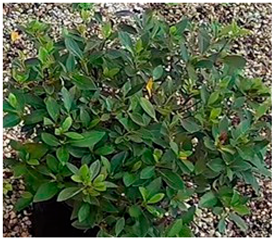
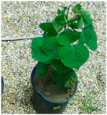
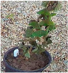
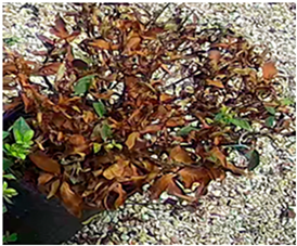
Figure 2 shows the raw plant images captured by the cameras. The image data were not suitable for image classification tasks due to varying image quality, excessive background information, and inconsistent sizes. To address the issues, we preprocessed the images using image processing tools and software such as Python libraries. The libraries implemented include Numpy (version 2.0.2), PyTorch (version 2.8.0), TensorFlow (version 2.19.0), Pandas (version 2.2.2), Keras (version 3.10.0), Matplot library (version 3.10.0), Pillow (version 11.3.0) and Scikit-learn (version 1.6.1). The images were cropped to focus on the region of interest (RoI) and resized to 300 × 300 pixels. Augmentation methods such as flipping and rotating were also employed. After preprocessing, a total of 4000 images were selected and categorized into six groups. There are three plant health conditions for each type of plant, which are bad plant health, medium plant health, and good plant health. As seen in Table 1 and Table 2, the six classifications comprise the azalea plant (bad, medium, and good) and Chinese tallow (bad, medium, and good). A data set was carefully selected to ensure a variety in plant structure, orientation, and light reflection.
For sensor data, the initial data normalization step was to screen the datasets for missing values and anomalies using big data visualization tools. To optimize the data set and eliminate redundancy, only 45 days after treatments, when the effects were most experienced, were included. Variations in moisture and fertility were determined and analyzed to better understand how the plant responds to treatments, taking into account that the moisture level influences the electrical conductivity of the soil. The fertility reading between the Chinese Tallow and the Azalea were examined carefully; after which the Azalea was excluded from the final training because of its inconsistencies. Min-Max-Scaler normalizer was used to scale the data features between 0 and 1. Sensors measure and thus equate soil electrical conductivity with fertility. If the soil is more fertile, it will contain more electrolytes. However, this does not directly imply that all high electrical conductivity situations mean fertility or that the soil condition is favorable for plant growth. High soil moisture and harmful chemical induction can also increase the EC level of the soil, which does not equal fertility or favorable plant conditions. For this reason, we analyzed the variations between soil fertility and moisture, to focus on the effects of the treatments alone. Since soil electrical conductivity fluctuates over time, we cannot assume a fixed ‘medium’ value. As seen in Table 3, class 0 describes the situation where there is negligible variation with 0% (healthy soil condition), while class 1 signifies the level of variation 100% (unhealthy soil condition). The data sets were strategically divided into training (70%), validation (20%) and testing (10%) to ensure balance between stress categories.

2.4. Structure of Proposed Model

Neural networks make it possible to analyze data in various formats such as high-resolution images and sensor data. ML models can track environmental factors, such as temperature fluctuations, moisture content, and fertility, as well as identify abnormal changes in plants caused by stressors [16]. As the depth of neural networks increases, its accuracy degrades quickly due to vanishing gradient, as the gradients will become too small during backpropagation [18,19]. To address this challenge, the ResNet model was selected for image processing while LSTM was selected for sensor data analysis. In previous trials, other architectures were implemented, including ResNet-50 and ResNet-18, which were presented at the Foundations of Process/Product Analytics and Machine Learning (FOPAM) 2023 conference. ResNet34 was selected to analyze camera images because it has fewer layers and parameters and requires less memory. ResNet34 also typically performs better with smaller datasets. Thus, it is faster to train and will generally be more suitable for edge computing and real-time processing. Additionally, an LSTM neural network was selected to analyze soil sensor data because it processes long-term dependencies in the data better than other RNNs. LSTM is also generally good at handling noisy, complex, and lengthy time series data. It is also flexible and can be combined with other models when expansion is desired for future studies.

2.4.1. ResNet Model

We implement a ResNet-34 architecture in TensorFlow. The network begins with a convolution layer with a 7 × 7 kernel ad output 64 channel, followed by batch normalization, ReLU activation, and the max-pooling layer. Its network contains several residual block (Basic Block) modules, which consists of two convolutional layers for each block. The block depth increases from 64 to 128, 256, and lastly 512. Dropout layers were added within the network layers to manage overfitting that may occur during the training process. Finally, a fully connected layer was implemented at the end of the network.
By default, this optimizer is set as Stochastic Gradient Descent (SGD). However, model allows flexible selection of optimizers like the Adam optimization algorithm. The training was carried out on TensorFlow-GPU environment using Keras framework. The cross-entropy loss function was implemented to calculate the loss between the predictions and the true labels. For training, step decay learning rate was reduced by a factor of 0.3 every 10 epochs, for a reduction factor of 0.3. The learning rate was set to 0.001 while the weight decay for regularization was set to 0.01. Early stopping which terminates the training if there was no improvement in the model performance was implemented. Stochastic Gradient Descent (SGD) is the default optimizer, but the model allows flexible selection of optimizers like Adam optimization algorithm to be utilized instead. The training was carried out on TensorFlow-GPU environment using Keras framework. Table 4 contains the parameters used for the ResNet model.
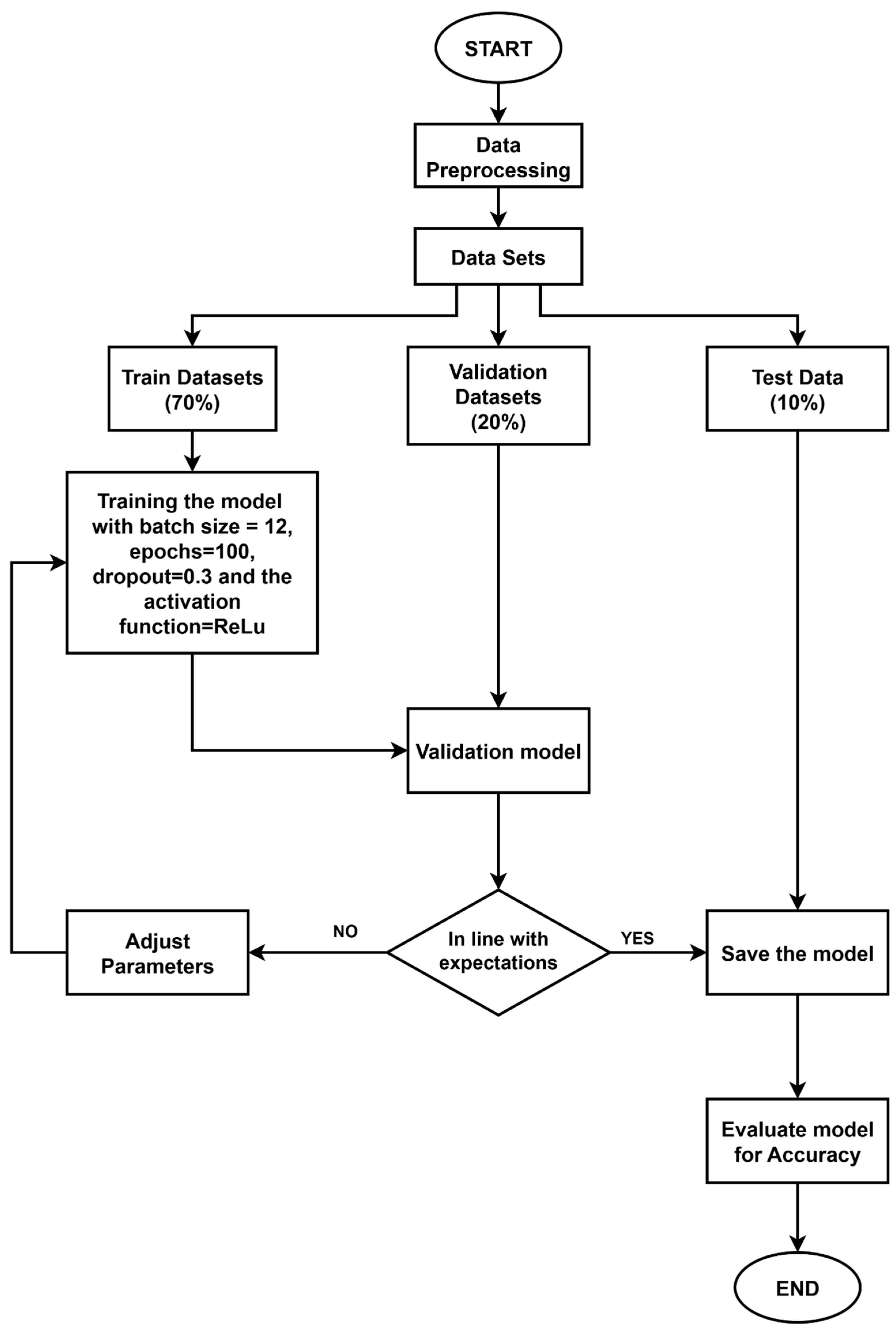
Figure 3 shows the step-by-step process for image processing. After preprocessing and splitting the datasets in training, validation and test sets, the model was trained on 70% (training set) of the total datasets. After the training process, the validation data sets validate the model. If the validation performance did not meet the expected criteria, the parameters are adjusted, and the training repeated. When satisfactory performance was met, the model was saved. At desired performance, the test data sets were used to further evaluate how accurate the model can classify unseen data.

2.4.2. Long Short-Term Memory (LSTM) Neural Network

LSTM neural networks are a specific kind of Recurrent Neural Network (RNN) that are good at handling long-term dependencies in time series data [20]. LSTMs were first introduced by Sepp Hechreiter and Jurgen Schimidhuber to solve vanishing gradient issues that occur in conventional RNNs [21]. The LSTM architecture uses a chain architecture that is composed of four interacting layers [22]. Unlike the RNN, the LSTM has three types of gates: input, forget and output gates. The information passes through the memory unit called the cell state. The cell state has a sigmoid activation function that regulates whether to store, update or erase and incoming data. The gates perform matrix multiplications with distinct set of weights to filter data effectively [22].
The LSTM neural network was implemented in Python using TensorFlow (version 2.19.0), along with its supporting libraries. A Keras LSTM with a single LSTM layer with 50 units was implemented. Its input includes timesteps, features, and batch size. This is passed through the LSTM layer, then followed by a dropout layer. To improve generalization, a dropout rate of 0.3 was used. The optimizer used for the training is the Adam optimizer with a learning rate of 0.001, while the batch size used for the training was 32. The hyperparameters were tuned empirically using validation performance as a guide. Cross-validation was performed across several sets to ensure robustness. Table 5 contains the parameters used for the LSTM model.

2.5. Performance Evaluation

Several evaluation techniques were employed in evaluating the performance and effectiveness of the models. These methods include accuracy, precision, recall, and F1-score. Accuracy is calculated by taking the ratio of true or correct predictions to the total number of predictions made by the model. Precision is measured as the proportion of the number of true positives compared to the number of positives predictions. Recall is the metric that checks the number of true positive classifications against actual positive occurrences. Finally, the F1 score is calculated by taking the harmonic mean value of precision and recall. The following equations shown in (1) to (4) are the mathematical representations of the performance matrices.
A c c u r a c y = T P + T N T P + T N + F P + F N
P r e c i s i o n = T P T P + F P
R e c a l l = T P T P + F N
F 1 s c o r e = 2 × P r e c i s i o n × R e c a l l P r e c i s i o n + R e c a l l
  • TP: True Positive
  • TN: True Negative
  • FP: False Positive
  • FN: False Negative

3. Results

3.1. ResNet34 Model Results

The classification report for the six different classifications can be seen in Table 6. This report provides the precision, recall, and F1 score of the model. The evaluation scores show that the model achieved high performance in the six classes, with 96% accuracy of the test data sets.
As seen in Figure 4, the accuracy graph showed an increasing trend, while the loss graph showed a decreasing trend over the epoch. The model started to stabilize after Epoch 70. Although the background of the image was not removed, the model effectively identified the object of interest within the noisy data, further demonstrating the effectiveness of the model.
The confusion matrix as seen in Figure 5 displays the results of a model’s classification performance. The difference in the number of samples in each class reflects the variability of the plants, rather than the inconsistency of the data. For example, Chinese tallow plants have diverse branching structures, which result in different image samples. Similarly, images of plants with about 80% brown leaves and those that had completely shed their leaves were classified under Azalea Bad Plant health (Class 2), thus creating multiple samples within the same class. However, with the variety of plant shapes and structures, the model correctly classified most of the instances with a few incorrect classifications.

3.2. LSTM Model Results

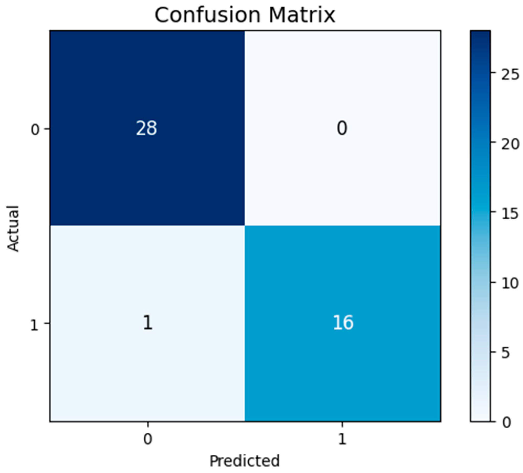
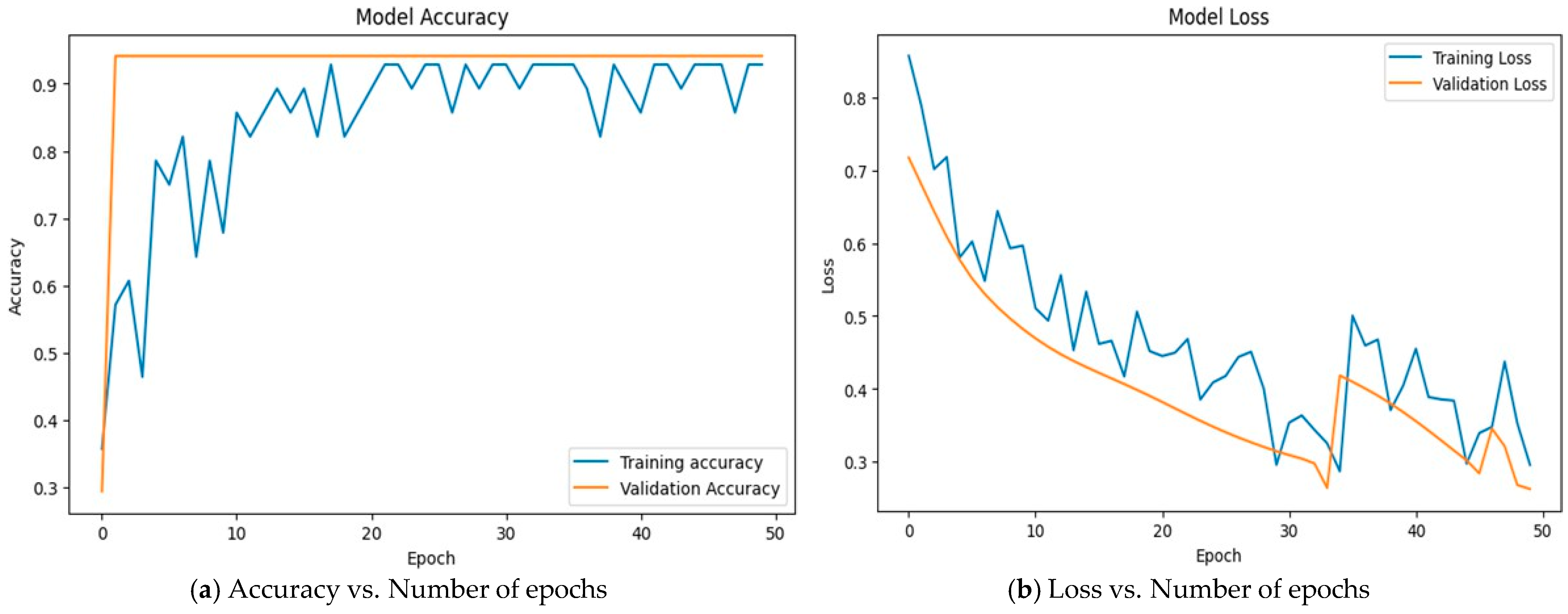
In this training process, the LSTM architecture was redefined. We deployed an LSTM architecture that had a two-layer design earlier, which has a 64-unit and a 32-unit LSTM. The LSTM model did not perform well as overfitting was observed. The LSTM model was simplified to a single layer with 50 units and reduced the epoch size to 50, to prevent overfitting and reduce computation without degrading the model performance, since the accuracy did not change after epoch 40 in the first experiment. The model achieved a classification accuracy of 97.8% in the test set. Based on the LSTM confusion matrix seen in Figure 6, the model correctly classified the instances with only one incorrect classification. As seen in Figure 7, at Epoch 50 the loss is less than 40% unlike the first experiment, which was over 50%.

3.3. Predictive Analysis Using Soil Data

This section discusses the predictive analysis performed using the Chinese tallow soil data under acetic acid and salt treatments. As mentioned earlier in this paper, soil moisture influences soil EC; therefore, these are major parameters considered for this analysis. Variations between these two parameters were determined and normalized between 0 and 1 to allow direct comparison between treatments.

3.3.1. Acetic Acid Variation Results

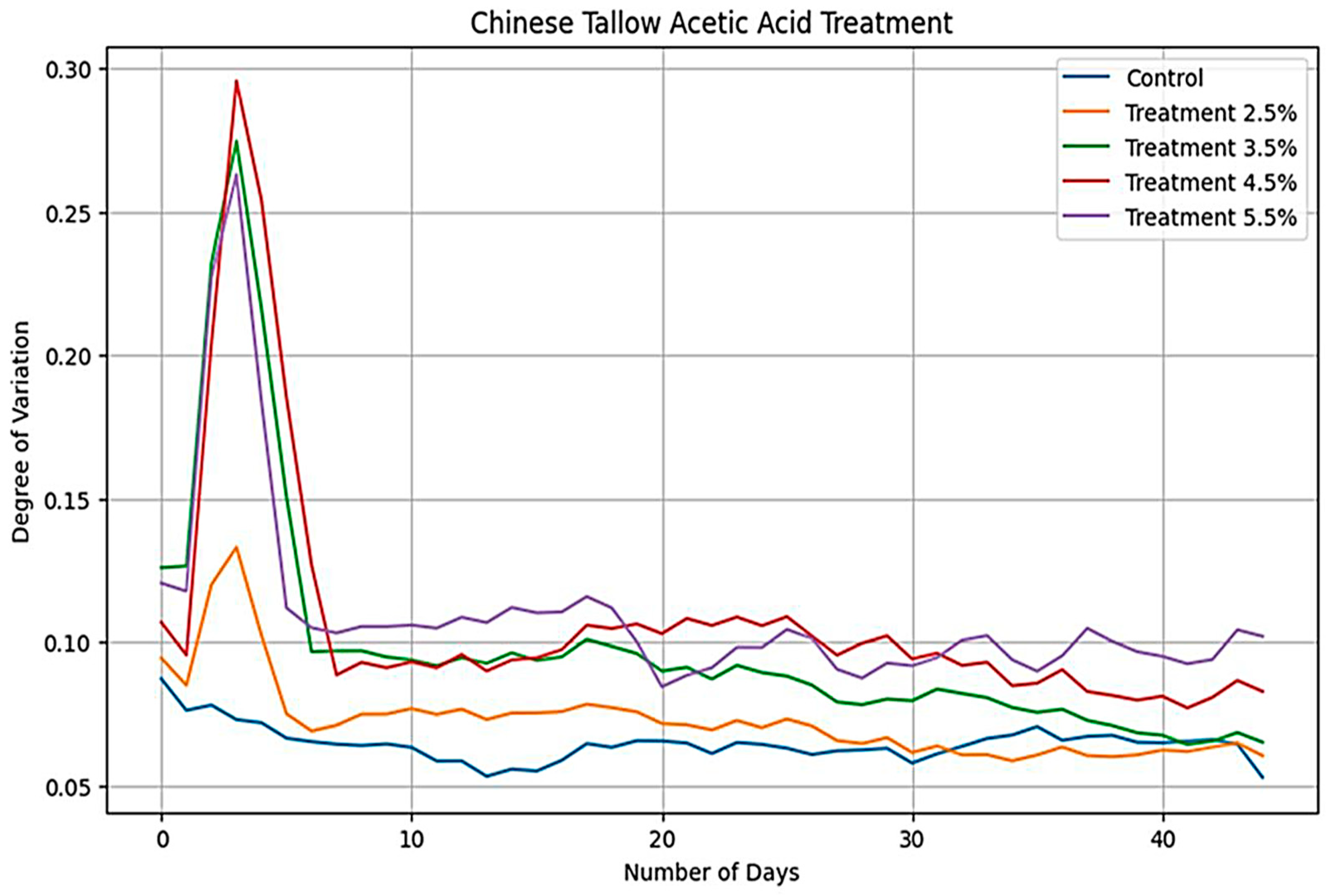
Using the soil variation in the control plant group as a reference point to determine which soil condition represents abnormal and extreme responses. However, the other four groups of treatment concentrations showed extreme responses in the first 10 days after treatments. The plant group treated with 3.5%, 4.5% and 5.5% acetic acid concentrations exhibited visible changes (such as fatigued leaves) after 5 days. The plant group with 2.5% acetic acid treatment, started showing visual changes (such as fatigued leaves) after 7 days. As shown in Figure 8, the control plant remained below the 10% variation throughout the 45-day period of this analysis, and all treated plants showed a high degree of variation within the first 10 days but the soil conditions stabilized after this initial spike. However, once the plant leaves started to change color after treatments were applied, those changes were irreversible.

3.3.2. Sodium Chloride Variation Results

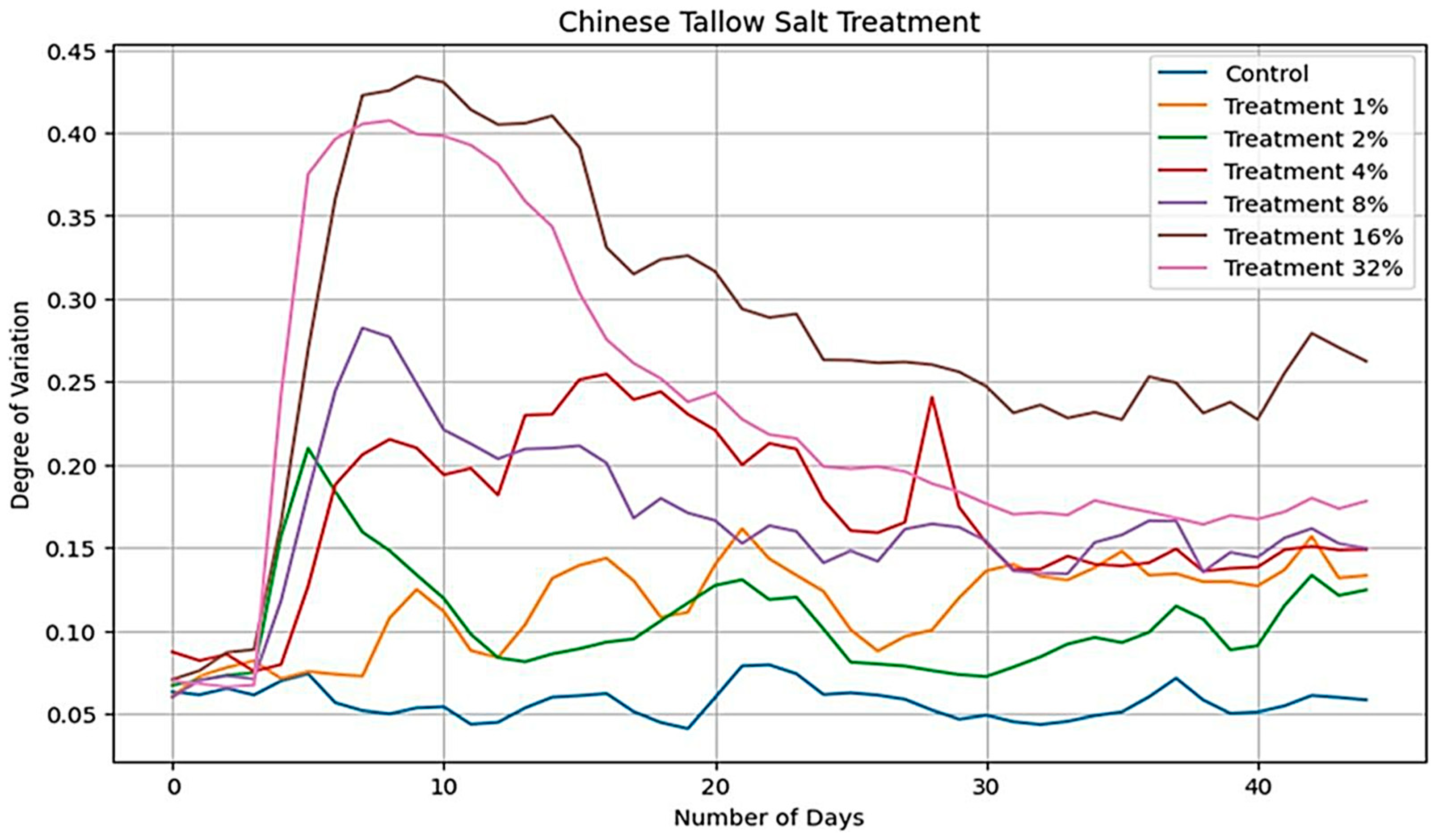
In Figure 9, all plant treatment groups, except the control plants, exhibited extreme responses to treatments. The plant groups with 32% and 16% NaCl treatment showed leaf color changes after 5 days after applying the treatments. Although the plant leaves of the 32% and 16% treatments did not recover from their treatments, the group of plants treated with 8% of NaCl gradually recovered and produced new green leaves 10 days after applying the treatment. Meanwhile, plants with NaCl treatments of 4%, 2% and 1% did not show visual changes during the experimental period. As shown in Figure 9, the control plant remained below the 10% variation throughout the 45-day period of this analysis, and all treated plants showed a high degree of variation within the first 10 days but the soil conditions did not stabilize after this initial spike.

4. Discussion

The goal of this research project was to apply abiotic stressors to several types of plants to see what levels of stressors degraded the plant’s health. Moreover, machine learning models were used to determine how accurately they could evaluate and classify the results. Therefore, known and established models were used. These models provided very accurate results (>90%). However, with any study, additional research can always be performed to expand and complement the original study. Additional plant species can be evaluated under the same stimuli. Specifically, different plants can be used, weeds can be evaluated, and crops can also be explored to determine how healthy they are after applying various levels of salt and acetic acid. Moreover, different stimuli can also be evaluated. For example, various abiotic stimuli (such as specific chemicals or different types of radiation) as well as biotic stimuli (such as microbial pathogens) or a combination of these stimuli could be evaluated.
This research study utilizes different machine learning models (ResNet34 and LSTM) on different modes of data (image and sensor) from dual species (tree and shrub) after applying different stressors (salt and acetic acid). Thus, this research is unique and goes beyond published research by using technology to broaden the scope of evaluation and understanding of plant responses to external stimuli across plant types. Although no other study is identical to this study, some meaningful comparisons can be made to results from similar studies [39,40,41,42,43].
In a paper by Do et al., images from unmanned aerial vehicles (UAVs) and sensor data from a chlorophyll meter, spectroradiometer, and water potential meter were used to assess citrus plant health through linear regression and a CNN ML models [39]. Due to the wavelength range of the particular measurements, results show that the ML models are able to predict chlorophyll values better than water potential or normalized difference vegetative index (NDVI). Results also show detection of significant nitrogen and water stress, but root mean square error (RMSE) is reported instead of accuracy, so direct comparisons between those results and results from the current study cannot be made. A research paper by Atanasov et al., utilized a spectrum colorimeter to measure the leaf color, a frequency-domain sensor to measure soil water content, and a soil temperature sensor. The authors used various ML models (Zero Rule, Linear Regression, Locally Weighted Learning, M5P Model Tree, Support Vector Machine, Decision Tree, and Multilayer Perceptron) to assess soil moisture based on leaf color. Of these models, the Decision Tree Regression Model produced the best results for RMSE, but again accuracy was not reported, so a direct comparison is difficult. Results also demonstrate that tomato leaf color is correlated to soil moisture and soil temperature [40]. Additionally, this research does not use images of the plant but uses a colorimeter and young leaves perform better than older leaves. Studies by Wang et al. and Tian et al., assess plant health through multispectral leaf images [41,42]. A multitude of ML algorithms were assessed such as Epsilon-Support Vector Regression (e-SVR), Elastic–Net Regularization Regression (Elastic-Net), Partial Least Squares Regression (PLSR), Random Forest Regression (RF) [41], as well as Extreme gradient boosting (XGBoost), gradient boosting decision tree (GBDT), random forest (RF), radial basis function neural network (RBFNN) and support vector regression (SVR) [42]. Although both studies report RMSEs for the models, XGBoost provided an accuracy of 92.9% in assessing plant health from aboveground biomass derived from multispectral images [41]. It is noted that the accuracy reported herein is higher and it includes soil analysis whereas the results reported by Wang et al., and Tian et al. do not assess soil health [41,42]. Finally, a study by Shafi et al., used a multimodal approach to assessing crop health by using multispectral imaging and sensor data (soil temperature, soil moisture, air temperature, air moisture [or humidity]) [43]. ML models included Naive Bayes (NB), Support Vector Machine (SVM) and seven Neural Networks (NN) with various hyperparameters, hidden layers and activation functions. The results were excellent and 98% accuracy was achieved, but only one plant type was evaluated (wheat crops) and only 2 classification levels were used (instead of 3 levels). Thus, the approach used in the current research project is unique and has great potential to enhance industrial farming applications by integrating early stress alerts systems and management decisions; however, the accuracy of this approach may improve through multimodal ML evaluation.
This research study is step forward in advancing smart automated agriculture. But again, the research is not complete, and additional studies are needed to answer some important questions. Because the datasets were limited for this study, randomization was utilized during the training process to produce more reliable model parameters. As demonstrated, the results were very accurate and acceptable. Additionally, k-fold cross-validation was performed to determine if results could be better. This k-fold analysis reduced accuracy from 0.94 to 0.68. Furthermore, because multispectral image processing can provide data beyond the visible spectrum, it may detect subtle plant changes and thus could be incorporated into the system to enhance performance. Finally, the ResNet and LSTM models (and others) could be integrated into a hybrid or multimodal decision system where results can be synthesized to provide a unified decision support system.
Regarding k-fold cross-validation, research results are mixed. Some researchers report that it performs well [44], and others demonstrate that it does not [45]. Additional research reports that there are many factors that can affect performance such as the value of k and the complexity of the data [46,47]. Regarding multispectral imaging, there are many papers that demonstrate the benefits of using these types of imaging systems with ML algorithms [48,49]. However, the high cost of these systems will limit their use, and additional research is still needed because various factors such as environmental conditions along with spectral and spatial resolution can affect performance [50,51]. Finally, regarding multimodal classification, research is showing that this approach is beneficial especially to determine the presence of stress and the reason for that stress [52,53]. As promising as this research is, factors such as the type of data (terrestrial images, satellite images, soil sensor data, environmental data, etc.) as well as what type of algorithms (RNN, CNN, DNN) and hybrid model architectures need to be researched to determine these answers [43,54,55,56].
One objective of this study was to determine if image-based and sensor-based ML models could detect deterioration or decline in plant health. Thus, selecting reliable and trusted ML algorithms was the primary concern rather than testing or evaluating novel architectures. Therefore, the analysis or classification of plant images was performed using a ResNet-34 ML algorithm. Likewise, analysis of IoT soil sensor data was performed using an LSTM ML algorithm. Although there are many neural network architectures that can classify images, ResNet is widely used design and it generally outperforms other CNNs [57]. As a result, ResNet was chosen for this study. Additionally, there are many ResNet architectures (e.g., ResNet-18 and ResNet-50), but ResNet-34 was selected because of its accuracy and speed (it has more layers than ResNet-18 and thus is more accurate and it has fewer layers than ResNet-50 and thus is faster). Similarly, there are numerous ML algorithms for classification of time series data such as ARIMA and GRU. There are many papers suggesting that LSTM outperforms its counterparts when it comes to forecasting future events [58,59] but some research also suggest that LSTM is superior to classical neural networks such as Decision Tree, SVM, Logistic Regression, and K-means [60].
A collective analysis was carried out on abiotic stressed plants using both ResNet-34 and LSTM models to determine the precision, recall, and F-1 score related to plant health status and soil conditions. These evaluations were performed using the weighted scores in order balance the datasets, as some plant health classes had multiple visual variations. By reporting the weighted scores, the evaluation would provide a fair assessment of the model performance under class imbalance. ResNet-34 achieved weighted scores of 0.96 for precision, recall and F1 score, thereby showing how reliable the model is in performing classification and detection tasks. The precision, recall and F-1 score for LSTM was also very good achieving values of 0.89, 0.94, and 0.91, respectively. These results confirm that both models were effective in capturing physiological changes when all plant classes are weighted. In addition to being accurate, once the models are trained, they are relatively rapid in providing real-time results. The training time for the LSTM model took approximately 7 s and the inference time took approximately 2 msec. The training time for the ResNet34 model took approximately 2.5 h, and the inference time took a maximum of 60 s.
It is noted that during this research, various challenges were encountered. The issues centered on sensor battery failure, sensor noise, plant rooting issues, and variable lighting conditions that affects the video/image quality and usability. For example, the sensor images captured during late hours of the day were too dark or were affected by fluctuating illumination which affected the pixels and color representation of the plants, making it difficult for the model to learn and classify the plants correctly. To help meet the objective of this study, optimal images were applied to the ML model. For the IoT sensors, several cases of electrical instability were observed, where the sensors either stopped reporting a certain parameter or went completely silent for hours within a day. To solve these challenges, more frequent checks and replacements were performed, and multiple redundant sensors were used in each treatment group to ensure reliability. Sections of data with missing reading or lower quality images were removed during preprocessing. However, to provide greater flexibility for the model, and meet real world scenarios, it is better to reduce data preprocessing. This additional research, necessary refinements, and corresponding advances may not only improve model performance and reliability in real world performance but also bring the research closer to practical application and long-term improvements in crop productivity.

5. Conclusions

This research explored the utilization of deep learning architectures for plant health analysis under different external stressors integrating image analysis and sensor analysis. ResNet-34 and LSTM neural networks were implemented for the different data types (image and sequential data). Both neural network models achieved high accuracy level, with the ResNet-34 reaching 96% accuracy for image classification and the LSTM model reaching 97.8% accuracy for soil data analysis. This demonstrates the successful application of machine learning in analyzing and detecting plants responses to external abiotic stimuli (salt and acetic acid).
This study was conducted in a greenhouse to keep a controlled environment. Although the results are promising, this research is limited to two plant species, which limits generalization, and should be considered as an initial step rather than a conclusive solution for agriculture. Further studies should be conducted to broaden the data sets and incorporate other types of stressors to improve robustness. Despite these limitations, the study demonstrates the potential of machine learning to be used as a tool for a non-destructive analysis in precision agriculture.

Author Contributions

Conceptualization, F.L., Y.I., Y.Q., W.G., J.L.; methodology, F.L., Y.I., F.D., E.E.D., Y.Q., W.G., J.L., F.L.; software, C.A., F.D., J.L.; validation, C.A., Y.I., E.E.D., Y.Q., W.G., J.L., F.L.; formal analysis, C.A., Y.I., E.E.D., Y.Q., W.G., J.L., F.L.; investigation, C.A., Y.I., F.D., E.E.D., Y.Q., W.G., J.L., F.L.; writing—original draft preparation, C.A.; writing—review and editing, C.A., F.L.; project administration, F.L.; funding acquisition, F.L. All authors have read and agreed to the published version of the manuscript.

Funding

This work was funded by a research grant from the United States Government under contract number 2021-21061700002.

Institutional Review Board Statement

Not applicable.

Informed Consent Statement

Not applicable.

Data Availability Statement

Data cannot be made public, due to privacy policy by the funding agency. The ML codes can be found on GitHub at https://github.com/Chinwe-A2022 (accessed on 1 September 2025).

Conflicts of Interest

The authors declare no conflict of interest.

Abbreviations

The following abbreviations are used in this manuscript:
CNNConvolutional Neural Network
RNNRecurrent Neural Network
DNNDeep Neural Network
GRUGated Recurrent Unit
ARIMAAutoRegressive Integrated Moving Average
ResNetResidual Network
LSTMLong Short-Term Memory
MLMachine Learning
RFRandom Forest
SVMSupport Vector Machine
ECElectrical Conductivity
SGDStochastic Gradient Descent
GPUGraphics Processing
CPUCentral Processing Unit
NARXNonlinear Autoregressive Exogenous

References

  1. Hemathilake, D.M.K.S.; Gunathilake, D.M.C.C. Agricultural productivity and food supply to meet increased demands. In Future Foods; Academic Press: Cambridge, UK, 2022; pp. 539–553. [Google Scholar] [CrossRef]
  2. Vezzani, F.M.; Anderson, C.; Meenken, E.; Gillespie, R.; Peterson, M.; Beare, M.H. The importance of plants to development and maintenance of soil structure, microbial communities and ecosystem functions. Soil Tillage Res. 2018, 175, 139–149. [Google Scholar] [CrossRef]
  3. Velmourougane, K.; Blaise, D. Soil health, crop productivity and sustainability challenges. In Sustainability Challenges in the Agrofood Sector; John Wiley & Sons: Hoboken, NJ, USA, 2017; pp. 509–531. [Google Scholar] [CrossRef]
  4. Minhas, P.S.; Rane, J.; Pasala, R.K. Abiotic stresses in agriculture: An overview. In Abiotic Stress Management for Resilient Agriculture; Springer: Singapore, 2017; pp. 3–8. [Google Scholar] [CrossRef]
  5. Nicolopoulou-Stamati, P.; Maipas, S.; Kotampasi, C.; Stamatis, P.; Hens, L. Chemical pesticides and human health: The urgent need for a new concept in agriculture. Front. Public Health 2016, 4, 148. [Google Scholar] [CrossRef] [PubMed]
  6. Kudo, T.; To, T.K.; Kim, J.-M. Simple and universal function of acetic acid to overcome the drought crisis. Stress Biol. 2023, 3, 15. [Google Scholar] [CrossRef] [PubMed]
  7. Mahmud, S.; Kamruzzaman, M.; Bhattacharyya, S.; Alharbi, K.; Abd El Moneim, D.; Mostofa, M.G. Acetic acid positively modulates proline metabolism for mitigating PEG-mediated drought stress in maize and Arabidopsis. Front. Plant Sci. 2023, 14, 1167238. [Google Scholar] [CrossRef] [PubMed]
  8. Machado, R.M.A.; Serralheiro, R.P. Soil salinity: Effect on vegetable crop growth. Management practices to prevent and mitigate soil salinization. Horticulturae 2017, 3, 30. [Google Scholar] [CrossRef]
  9. Rahman, M.M.; Keya, S.S.; Sahu, A.; Gupta, A.; Dhingra, A.; Tran, L.S.P.; Mostofa, M.G. Acetic acid: A cheap but chief metabolic regulator for abiotic stress tolerance in plants. Stress Biol. 2024, 4, 34. [Google Scholar] [CrossRef]
  10. Gondek, M.; Weindorf, D.C.; Thiel, C.; Kleinheinz, G. Soluble salts in compost and their effects on soil and plants: A review. Compost. Sci. Util. 2020, 28, 59–75. [Google Scholar] [CrossRef]
  11. Munns, R.; Tester, M. Mechanisms of salinity tolerance. Annu. Rev. Plant Biol. 2008, 59, 651–681. [Google Scholar] [CrossRef]
  12. Ahmed, I.; Yadav, P.K. A systematic analysis of machine learning and deep learning based approaches for identifying and diagnosing plant diseases. Sustain. Oper. Comput. 2023, 3, 100–110. [Google Scholar] [CrossRef]
  13. Garofalo, S.P.; Ardito, F.; Sanitate, N.; De Carolis, G.; Ruggieri, S.; Giannico, V.; Rana, G.; Ferrara, R.M. Robustness of Actual Evapotranspiration Predicted by Random Forest Model Integrating Remote Sensing and Meteorological Information: Case of Watermelon (Citrullus lanatus, (Thunb.) Matsum. & Nakai, 1916). Water 2025, 17, 323. [Google Scholar] [CrossRef]
  14. Sujatha, R.; Krishnan, S.; Chatterjee, J.M.; Gandomi, A.H. Advancing plant leaf disease detection integrating machine learning and deep learning. Sci. Rep. 2025, 15, 11552. [Google Scholar] [CrossRef] [PubMed]
  15. van Dijk, A.D.J.; Kootstra, G.; Kruijer, W.; de Ridder, D. Machine learning in plant science and plant breeding. iScience 2021, 24, 101890. [Google Scholar] [CrossRef]
  16. Rico-Chávez, A.K.; Franco, J.A.; Fernandez-Jaramillo, A.A.; Contreras-Medina, L.M.; Guevara-González, R.G.; Hernandez-Escobedo, Q. Machine Learning for Plant Stress Modeling: A Perspective towards Hormesis Management. Plants 2022, 11, 970. [Google Scholar] [CrossRef]
  17. Tran, D.; Dutoit, F.; Najdenovska, E.; Wallbridge, N.; Plummer, C.; Mazza, M.; Raileanu, L.E.; Camps, C. Electrophysiological assessment of plant status outside a Faraday cage using supervised machine learning. Sci. Rep. 2019, 9, 17073. [Google Scholar] [CrossRef]
  18. Jung, D.-H.; Kim, H.S.; Jhin, C.; Kim, H.-J.; Park, S.H. Time-serial analysis of deep neural network models for prediction of climatic conditions inside a greenhouse. Comput. Electron. Agric. 2020, 173, 105402. [Google Scholar] [CrossRef]
  19. Sumathi, P.; Karthikeyan, V.V.; Kavitha, M.S.; Karthik, S. Improved Soil Quality Prediction Model Using Deep Learning for Smart Agriculture Systems. Comput. Syst. Sci. Eng. 2023, 45, 1545–1559. [Google Scholar] [CrossRef]
  20. Islam, M.R.; Oliullah, K.; Kabir, M.M.; Alom, M.; Mridha, M.F. Machine learning enabled IoT system for soil nutrients monitoring and crop recommendation. J. Agric. Food Res. 2023, 14, 100880. [Google Scholar] [CrossRef]
  21. Grunwald, S.; Murad, M.O.F.; Farrington, S.; Wallace, W.; Rooney, D. Multi-Sensor Soil Probe and Machine Learning Modeling for Predicting Soil Properties. Sensors 2024, 24, 6855. [Google Scholar] [CrossRef]
  22. Panchal, A.V.; Patel, S.C.; Bagyalakshmi, K.; Kumar, P.; Khan, I.R.; Soni, M. Image-based plant diseases detection using deep learning. Mater. Today Proc. 2023, 80, 3500–3506. [Google Scholar] [CrossRef]
  23. Dolatabadian, A.; Neik, T.X.; Danilevicz, M.F.; Upadhyaya, S.R.; Batley, J.; Edwards, D. Image-based crop disease detection using machine learning. Plant Pathol. 2025, 74, 18–38. [Google Scholar] [CrossRef]
  24. Thiagarajan, J.D.; Kulkarni, S.V.; Jadhav, S.A.; Waghe, A.A.; Raja, S.P.; Rajagopal, S.; Poddar, H.; Subramaniam, S. Analysis of banana plant health using machine learning techniques. Sci. Rep. 2024, 14, 15041. [Google Scholar] [CrossRef] [PubMed]
  25. Elsherbiny, O.; Elaraby, A.; Alahmadi, M.; Hamdan, M.; Gao, J. Rapid grapevine health diagnosis based on digital imaging and deep learning. Plants 2024, 13, 135. [Google Scholar] [CrossRef]
  26. Chug, A.; Bhatia, A.; Singh, A.P.; Singh, D. A novel framework for image-based plant disease detection using hybrid deep learning approach. Soft Comput. 2023, 27, 13613–13638. [Google Scholar] [CrossRef]
  27. Albahli, S. AgriFusionNet: A Lightweight Deep Learning Model for Multisource Plant Disease Diagnosis. Agriculture 2025, 15, 1523. [Google Scholar] [CrossRef]
  28. Tian, S.; Huang, W.; Hu, J.; Wang, H.; Zhang, Z.; Xu, L.; Li, J.; Sun, Y. Exploring the frontiers of plant health: Harnessing NIR fluorescence and surface-enhanced Raman scattering modalities for innovative detection. Chin. Chem. Lett. 2025, 36, 110336. [Google Scholar] [CrossRef]
  29. Hossain, N.I.; Tabassum, S. A hybrid multifunctional physicochemical sensor suite for continuous monitoring of crop health. Sci. Rep. 2023, 13, 9848. [Google Scholar] [CrossRef] [PubMed]
  30. Tussupov, J.; Yessenova, M.; Abdikerimova, G.; Aimbetov, A.; Baktybekov, K.; Murzabekova, G.; Aitimova, U. Analysis of formal concepts for verification of pests and diseases of crops using machine learning methods. IEEE Access 2024, 12, 19902–19910. [Google Scholar] [CrossRef]
  31. Rahu, M.A.; Chandio, A.F.; Ali, S.M. Machine Learning Overview in Agriculture. J. Appl. Eng. Technol. 2022, 6, 28–39. [Google Scholar] [CrossRef]
  32. Benos, L.; Tagarakis, A.C.; Dolias, G.; Berruto, R.; Kateris, D.; Bochtis, D. Machine Learning in Agriculture: A Comprehensive Updated Review. Sensors 2021, 21, 3758. [Google Scholar] [CrossRef]
  33. Liu, J.; Wang, X. A multimodal framework for pepper diseases and pests detection. Sci. Rep. 2024, 14, 28973. [Google Scholar] [CrossRef]
  34. He, K.; Zhang, X.; Ren, S.; Sun, J. Deep residual learning for image recognition. In Proceedings of the 2016 IEEE Conference on Computer Vision and Pattern Recognition (CVPR), Las Vegas, NV, USA, 27–30 June 2016; pp. 770–778. [Google Scholar] [CrossRef]
  35. Wu, W.; Huo, L.; Yang, G.; Liu, X.; Li, H. Research into the application of ResNet in soil: A review. Agriculture 2025, 15, 661. [Google Scholar] [CrossRef]
  36. Hochreiter, S.; Schmidhuber, J. Long short-term memory. Neural Comput. 1997, 9, 1735–1780. [Google Scholar] [CrossRef]
  37. Lacy, F.; Ruiz-Reyes, A.; Brescia, A. Machine learning for low signal-to-noise ratio detection. Pattern Recognit. Lett. 2024, 179, 115–122. [Google Scholar] [CrossRef]
  38. Yang, C.; Gan, X.; Peng, A.; Yuan, X. ResNet based on multi-feature attention mechanism for sound classification in noisy environments. Sustainability 2023, 15, 10762. [Google Scholar] [CrossRef]
  39. Do, D.; Pham, F.; Raheja, A.; Bhandari, S. Machine learning techniques for the assessment of citrus plant health using UAV-based digital images. In Autonomous Air and Ground Sensing Systems for Agricultural Optimization and Phenotyping III; SPIE: Bellingham, DC, USA, 2018; Volume 10664, pp. 189–200. [Google Scholar] [CrossRef]
  40. Atanasov, S.; Harizanova-Petrova, B.; Petrova, R. Tomato leaf color as predictor of soil moisture value using machine learning techniques. Sci. Horiz. 2023, 2, 31–42. [Google Scholar] [CrossRef]
  41. Wang, Q.; Lu, X.; Zhang, H.; Yang, B.; Gong, R.; Zhang, J.; Jin, Z.; Xie, R.; Xia, J.; Zhao, J. Comparison of machine learning methods for estimating leaf area index and aboveground biomass of cinnamomum camphora based on UAV multispectral remote sensing data. Forests 2023, 14, 1688. [Google Scholar] [CrossRef]
  42. Tian, F.; Zhou, J.; Ransom, C.J.; Aloysius, N.; Sudduth, K.A. Estimating corn leaf chlorophyll content using airborne multispectral imagery and machine learning. Smart Agric. Technol. 2025, 10, 100719. [Google Scholar] [CrossRef]
  43. Shafi, U.; Mumtaz, R.; Iqbal, N.; Zaidi, S.M.H.; Zaidi, S.A.R.; Hussain, I.; Mahmood, Z. A multi-modal approach for crop health mapping using low altitude remote sensing, internet of things (IoT) and machine learning. IEEE Access 2020, 8, 112708–112724. [Google Scholar] [CrossRef]
  44. Gorriz, J.M.; Segovia, F.; Ramirez, J.; Ortiz, A.; Suckling, J. Is K-fold cross validation the best model selection method for Machine Learning? arXiv 2024, arXiv:2401.16407. [Google Scholar] [CrossRef]
  45. White, J.; Power, S.D. k-fold cross-validation can significantly over-estimate true classification accuracy in common EEG-based passive BCI experimental designs: An empirical investigation. Sensors 2023, 23, 6077. [Google Scholar] [CrossRef]
  46. Nti, I.K.; Nyarko-Boateng, O.; Aning, J. Performance of machine learning algorithms with different K values in K-fold cross-validation. Int. J. Inf. Technol. Comput. Sci. 2021, 13, 61–71. [Google Scholar] [CrossRef]
  47. Wieczorek, J.; Guerin, C.; McMahon, T. K-fold cross-validation for complex sample surveys. Stat 2022, 11, e454. [Google Scholar] [CrossRef]
  48. Gaikwad, S.; Tidke, S. Multi-spectral imaging for fruits and vegetables. Int. J. Adv. Comput. Sci. Appl. 2022, 13, 743–760. [Google Scholar] [CrossRef]
  49. Barjaktarovic, M.; Santoni, M.; Bruzzone, L. Design and verification of a low-cost multispectral camera for precision agriculture application. IEEE J. Sel. Top. Appl. Earth Obs. Remote Sens. 2024, 17, 6945–6957. [Google Scholar] [CrossRef]
  50. Haque, M.A.; Reza, M.N.; Ali, M.; Karim, M.R.; Ahmed, S.; Lee, K.D.; Khang, Y.H.; Chung, S.O. Effects of environmental conditions on vegetation indices from multispectral images: A review. Korean J. Remote Sens. 2024, 40, 319–341. [Google Scholar] [CrossRef]
  51. Waiphara, P.; Bourgenot, C.; Compton, L.J.; Prashar, A. Optical imaging resources for crop phenotyping and stress detection. In Environmental Responses in Plants: Methods and Protocols; Springer: New York, NY, USA, 2022; pp. 255–265. [Google Scholar] [CrossRef]
  52. Zandi, A.; Hosseinirad, S.; Zadeh, H.K.; Tavakolian, K.; Cho, B.-K.; Vasefi, F.; Kim, M.S.; Tavakolian, P. A systematic review of multi-mode analytics for enhanced plant stress evaluation. Front. Plant Sci. 2025, 16, 1545025. [Google Scholar] [CrossRef] [PubMed]
  53. El Sakka, M.; Ivanovici, M.; Chaari, L.; Mothe, J. A review of CNN applications in smart agriculture using multimodal data. Sensors 2025, 25, 472. [Google Scholar] [CrossRef] [PubMed]
  54. Garg, S.; Pundir, P.; Jindal, H.; Saini, H.; Garg, S. Towards a multimodal system for precision agriculture using IoT and machine learning. In Proceedings of the 2021 12th International Conference on Computing Communication and Networking Technologies (ICCCNT), Kharagpur, India, 6–8 July 2021; IEEE: Washington, DC, USA; pp. 1–7. [Google Scholar] [CrossRef]
  55. Shukla, R.; Dubey, G.; Malik, P.; Sindhwani, N.; Anand, R.; Dahiya, A.; Yadav, V. Detecting crop health using machine learning techniques in smart agriculture system. J. Sci. Ind. Res. 2021, 80, 699–706. [Google Scholar] [CrossRef]
  56. Singh, R.; Nisha, R.; Naik, R.; Upendar, K.; Nickhil, C.; Deka, S.C. Sensor fusion techniques in deep learning for multimodal fruit and vegetable quality assessment: A comprehensive review. J. Food Meas. Charact. 2024, 18, 8088–8109. [Google Scholar] [CrossRef]
  57. Prajwal, T.S.; Ilavarasi, A.K. A comparative study of RESNET-pretrained models for computer vision. In Proceedings of the 2023 Fifteenth International Conference on Contemporary Computing, Noida, India, 3–5 August 2023; pp. 419–425. [Google Scholar] [CrossRef]
  58. Siami-Namini, S.; Tavakoli, N.; Namin, A.S. A comparison of ARIMA and LSTM in forecasting time series. In Proceedings of the 2018 17th IEEE International Conference on Machine Learning and Applications (ICMLA), Orlando, FL, USA, 17–20 December 2018; IEEE: Washington, DC, USA; pp. 1394–1401. [Google Scholar] [CrossRef]
  59. Paliari, I.; Karanikola, A.; Kotsiantis, S. A comparison of the optimized LSTM, XGBOOST and ARIMA in Time Series forecasting. In Proceedings of the 2021 12th International Conference on Information, Intelligence, Systems & Applications (IISA), Chania Crete, Greece, 12–14 July 2021; IEEE: Washington, DC, USA; pp. 1–7. [Google Scholar] [CrossRef]
  60. Saifullah, S. Comparative Analysis of Long Short-Term Memory and Gated Recurrent Unit Models for Chicken Egg Fertility Classification Using Deep Learning. Eng. Proc. 2025, 87, 7. [Google Scholar] [CrossRef]
Figure 1. Flow chart summary of experimental design and analysis.
Applsci 15 10960 g001
Figure 2. Camera image of the plants during one of the experimental studies.
Applsci 15 10960 g002
Figure 3. Flowchart of the machine learning design processing for image analysis.
Applsci 15 10960 g003
Figure 4. Training performance of the ResNet34 model: (a) The graph shows the validation accuracy over the number of epochs; (b) The graph shows the training and validation loss over the number of epochs.
Applsci 15 10960 g004
Figure 5. Confusion matrix for ResNet34 classification.
Applsci 15 10960 g005
Figure 6. Confusion matrix for LSTM classification.
Applsci 15 10960 g006
Figure 7. Training performance of the LSTM model: (a) The graph shows the accuracy over the number of epochs; (b) The graph shows the loss over the number of epochs.
Applsci 15 10960 g007
Figure 8. Daily variation in acetic acid for Chinese tallow.
Applsci 15 10960 g008
Figure 9. Daily variation in salt for Chinese tallow.
Applsci 15 10960 g009
Table 1. Images of plants in various stages of health (good health, medium health, and bad health).
Azalea PlantChinese Tallow Plant
GoodApplsci 15 10960 i001Applsci 15 10960 i002
MediumApplsci 15 10960 i003Applsci 15 10960 i004
BadApplsci 15 10960 i005Applsci 15 10960 i006
Table 2. Designation for the ML classification and corresponding plant type and health status for the ResNet model.
ClassesImage Type
Class 0Azalea Good Plant health (AGP)
Class 1Azalea Medium Plant health (AMP)
Class 2Azalea Bad Plant health (ABP)
Class 3Chinese tallow Good Plant health (CGP)
Class 4Chinese tallow Medium Plant health (CMP)
Class 5Chinese tallow Bad Plant health (CBP)
Table 3. Designation for the ML classification and corresponding plant type and health status for the LSTM model.
ClassesSoil Status
Class 0Healthy Soil Condition
Class 1Unhealthy Soil Condition
Table 4. Experimental environment and parameter configuration of the ResNet model.
ParameterValues
Development environmentTensorFlow-GPU
Epochs100
Learning rate0.001
Weight decay0.01
Batch size12
Dropout0.3
Table 5. Experimental environment and parameters configuration of the LSTM model.
ParameterValues
Development environmentTensorFlow
Optimizer learning rateAdam 0.001
Epochs50
Batch size32
Dropout0.3
Table 6. Classification report for ResNet34 model for test datasets. Classes 0–2 represents Azaleas with good, medium and bad health status and classes 3–5 represents Chinese tallows with good, medium, and bad health status.
Azaleas Chinese Tallows
MetricClass 0Class 1Class 2Class 3Class 4Class 5
Precision1.001.000.980.970.910.96
Recall0.810.931.001.000.881.00
F1-score0.920.970.990.980.890.98
Support0.980.990.990.990.960.98
Disclaimer/Publisher’s Note: The statements, opinions and data contained in all publications are solely those of the individual author(s) and contributor(s) and not of MDPI and/or the editor(s). MDPI and/or the editor(s) disclaim responsibility for any injury to people or property resulting from any ideas, methods, instructions or products referred to in the content.