Towards Realistic Industrial Anomaly Detection: MADE-Net Framework and ManuDefect-21 Benchmark

Abstract

Visual anomaly detection (VAD) plays a critical role in manufacturing and quality inspection, where the scarcity of anomalous samples poses challenges for developing reliable models. Existing approaches primarily rely on unsupervised training with synthetic anomalies, which often favor specific defect types and struggle to generalize across diverse categories. To address these limitations, we propose MADE-Net (Multi-model Adaptive anomaly Detection Ensemble Network), an industrial anomaly detection framework that integrates three complementary submodels: a reconstruction-based submodel (SRAD), a feature embedding-based submodel (SFAD), and a patch discrimination submodel (LPD). A dynamic integration and selection module (ISM) adaptively determines the most suitable submodel output according to input characteristics. We further introduce ManuDefect-21, a large-scale benchmark dataset comprising 11 categories of electronic components with both normal and anomalous samples in the training and test sets. The dataset reflects realistic positive-to-negative ratios and diverse defect types encountered in real manufacturing environments, addressing several limitations of previous datasets such as MVTec-AD and VisA. Experiments conducted on ManuDefect-21 demonstrate that MADE-Net achieves consistent improvements in both detection and localization metrics (e.g., average AUROC of 98.5%, Pixel-AP of 68.7%) compared with existing methods. While MADE-Net requires pixel-level annotations for fine-tuning and introduces additional computational overhead, it provides enhanced adaptability to complex industrial conditions. The proposed framework and dataset jointly contribute to advancing practical and reproducible research in industrial anomaly detection.

1. Introduction

Industrial anomaly detection aims to identify unexpected deviations in manufacturing processes [1,2]. Automating this process not only ensures product quality but also improves production efficiency and reduces manual inspection costs. Despite considerable progress, existing studies still face challenges due to the scarcity of anomalous samples and the wide diversity of defect types. Most current approaches can be categorized into reconstruction-based methods [3,4,5,6] and embedding-based methods [7,8,9,10]. However, because they are predominantly trained in an unsupervised manner using only normal samples, their ability to generalize across heterogeneous anomaly types remains limited.

Different anomaly modeling strategies lead to complementary strengths and weaknesses. CutPaste-based methods primarily target structural anomalies, while embedding-based methods capture texture-related defects but may suffer from feature overlap and ambiguous decision boundaries under complex semantics. Reconstruction-based approaches can handle both structural and texture anomalies, but they often encounter “shortcut” learning, where the model overfits to background priors and fails to localize subtle defects. These limitations reveal a fundamental gap: no single unsupervised method can robustly handle diverse industrial defects that vary in morphology, texture, and spatial structure.

In addition, the lack of realistic benchmark datasets further constrains progress in industrial anomaly detection. Existing datasets, such as MVTec-AD [11] and VisA [12], are collected under controlled laboratory conditions, contain only normal samples for training, and lack negative examples for realistic evaluation. Datasets like MPDD [13] and MTD [14] focus on specific domains such as metallic or tiled surfaces, limiting their representativeness of real manufacturing variability. Consequently, the research community still lacks a comprehensive benchmark that reflects authentic defect diversity, component-level variation, and realistic positive-to-negative sample ratios.

To address these challenges, we propose the MADE-Net framework, which integrates multiple complementary unsupervised submodels and employs a dynamic integration strategy to adaptively select the most effective anomaly representation for each input. Furthermore, we introduce ManuDefect-21, a large-scale benchmark dataset of surface-mount technology (SMT) components, featuring both normal and defective samples with pixel-level annotations in both training and test sets. By combining a multi-model adaptive detection framework with a realistic industrial dataset, this study aims to advance the generalization and applicability of anomaly detection systems in practical manufacturing environments.

Our contributions to the scientific community are summarized as follows:

• Unified framework for heterogeneous anomalies: We propose MADE-Net, which systematically integrates reconstruction-, embedding-, and CutPaste-based paradigms to handle diverse anomaly structures within a single adaptive framework. This contributes a generalized perspective on model fusion for visual anomaly detection.
• Two-stage training paradigm: We design a combined unsupervised pretraining and supervised fine-tuning strategy that bridges the gap between synthetic and real anomalies. This approach provides a reproducible methodology for leveraging real annotated data in industrial inspection research.
• Benchmark dataset for realistic evaluation: We release ManuDefect-21, a large-scale dataset with 31,050 training and 13,321 testing samples across 11 electronic component types. It provides balanced positive-to-negative ratios and pixel-level annotations to promote reproducibility and fair comparison among future studies.
• Empirical validation and impact: Experiments on ManuDefect-21, MVTec-AD, and VisA show that MADE-Net achieves consistent improvements in both image-level and pixel-level detection metrics, offering a robust foundation for further academic research and industrial applications in automated inspection.

2. Related Work

Visual Anomaly Detection (VAD) is of great significance in manufacturing, quality inspection, and other industrial applications. The primary challenge is to accurately detect anomalies under conditions where only limited or exclusively normal samples are available. Current research in this field can be broadly divided into two categories: reconstruction-based approaches and embedding-based approaches. In addition, the authenticity and complexity of datasets are increasingly recognized as critical factors that influence both method performance and the overall research value.

2.1. Reconstruction-Based Method

Reconstruction-based methods operate on the fundamental principle of learning the generative mapping of normal images, with anomalies inferred from the discrepancies between the input and its reconstruction during inference. Early approaches, often based on Autoencoders (AEs) or Variational Autoencoders (VAEs) [15], suffer from the drawback that overly powerful reconstruction networks can inadvertently reproduce anomalous regions with high fidelity, leading to missed detections. To alleviate this limitation, later studies have proposed targeted enhancements: structure-aware mechanisms (e.g., AE-SSIM) to increase sensitivity to structural cues; sparse memory augmentation [16] to boost discriminative power for anomalous regions; and multi-scale reconstruction architectures [17,18] to capture discrepancies across multiple feature hierarchies.

Recent developments have extended the reconstruction paradigm from the image space to the semantic space. DSR [3] performs restoration in the feature space, elevating the reconstruction objective from pixels to features, while UTRAD [4] leverages a U-shaped Transformer architecture to reduce computational cost and improve segmentation quality. Generative Adversarial Networks (GANs) have also been integrated into reconstruction frameworks, as in AnoGAN [5] and subsequent multi-branch adversarial reconstruction methods, where adversarial training is employed to refine reconstruction fidelity. Although such methods excel in surface defect detection, they remain vulnerable to the “shortcut learning” problem, in which structurally or semantically misaligned anomalies are reconstructed with undesirably high fidelity, highlighting an open challenge in the field.

2.2. Embedding-Based Method

In contrast to reconstruction-based approaches that detect anomalies through reconstruction discrepancies, embedding-based methods operate from a feature discrimination perspective, modeling the distribution of normal samples in the feature space to identify anomalies. At inference time, anomaly scores are typically derived from the distance between a test sample and the modeled distribution of normal samples in the embedding space. Pioneering works such as Deep SVDD [7] and Patch SVDD [19] established the foundation by modeling normal distributions at the image and patch levels, respectively. Subsequent advances, including PaDiM [8] and GCPF [20], introduced multivariate Gaussian modeling and covariance estimation to achieve more precise detection and localization, while PatchCore [9] incorporated neighborhood-based distance computation to integrate local contextual cues, thereby improving robustness.

For example, DFR [21] adopted a regression-based alignment strategy to improve feature consistency by mapping features back to their original representations, thereby reducing variance among normal embeddings. STAD [22] employed an uninformed knowledge distillation framework to train a student model without direct anomaly exposure, improving efficiency while maintaining generalization, whereas MKDAD [23] leveraged multi-resolution knowledge distillation to better capture hierarchical features across different scales. The Dual-Attention Transformer [10] introduced both spatial and channel-wise attention to jointly refine feature representations, but also highlighted that most existing methods still struggle to capture high-level semantic structures, making them less effective for detecting complex logical anomalies. MSFlow [24] addressed this limitation by combining multi-scale features with a Normalizing Flow (NF) model, which explicitly models the distribution of normal embeddings and provides a more principled density estimation for anomaly detection.

2.3. Dataset Limitations and Real-World Challenges

The performance evaluation of industrial anomaly detection methods is highly dependent on benchmark datasets, yet the limitations of existing datasets have been widely recognized. For instance, MVTec AD [11] includes 15 object and texture categories with 3629 training and 1725 test images, but its training set contains only normal samples and the anomaly types are limited in diversity. VisA [12] offers 12 categories with 10,821 training and 9621 test images, yet most anomalies are collected in controlled laboratory settings, limiting their realism. MPDD [13] (1380 images) and MTD [14] (3 categories) are restricted to metallic or tile surfaces, which prevents them from reflecting the variety of anomalies and multi-source interferences encountered in real-world production. These limitations highlight the need for datasets with larger scale, diverse defect categories, and authentic industrial capture conditions—gaps that our proposed ManuDefect-21 dataset is specifically designed to address.

To mitigate data scarcity, a number of approaches have resorted to generating synthetic anomalies from existing datasets (e.g., CutPaste [25], DRAEM [26]). Nevertheless, OmniAL [27] has emphasized that such synthetic defects fail to capture the spatial variability and semantic richness of real anomalies, often causing sharp performance drops in deployment. Similarly, Few-Shot Part Segmentation [28] has shown that current datasets lack the capacity to model higher-order defects—such as logical inconsistencies and component misalignments—thereby constraining the transferability and general applicability of anomaly detection methods. These observations underscore the importance of developing datasets that more faithfully reflect real industrial scenarios, which is essential for advancing the practical adoption of industrial anomaly detection systems.

2.4. Comparative Analysis of Existing Methods

To provide a clearer overview of current approaches,

Table 1. Comparative summary of representative anomaly detection methods.

Method	Principle	Advantages	Limitations	Anomaly Type
AE/VAE [15]	Pixel-level reconstruction	Simple and efficient training	Reconstructs anomalies too well; poor generalization	Texture/structure
DSR [3]	Feature-level reconstruction	Better semantic representation	Sensitive to feature noise; limited localization	Texture/structure
PatchCore [9]	Nearest-neighbor embedding	Fast inference, high localization accuracy	Limited semantic generalization	Texture
PaDiM [8]	Multivariate Gaussian embeddings	Low computational cost	Assumes unimodal normal distribution	Texture
STAD [22]	Knowledge distillation	High efficiency; avoids anomaly exposure	May lose discriminative features	Structure
CutPaste [25]	Synthetic anomaly pretext	Data-efficient training	Limited realism of generated anomalies	Structural
MSFlow [24]	Normalizing flow-based modeling	Explicit feature density estimation	High training cost; complex implementation	Texture/logical

summarizes representative visual anomaly detection (VAD) methods from both reconstruction-based and embedding-based paradigms. The table compares them in terms of methodological principles, target anomaly types, key advantages, and existing limitations.

2.5. Analytical Discussion and Motivation

Despite remarkable progress, existing VAD approaches still exhibit common limitations. First, reconstruction-based methods often struggle with the “shortcut reconstruction” phenomenon, where abnormal regions are inadvertently restored due to overfitting. Second, embedding-based methods, though efficient, tend to exhibit feature overlap between normal and anomalous patterns, reducing discriminative reliability under complex industrial conditions. Third, CutPaste-style or flow-based methods, while effective in simulation, remain constrained by their dependence on synthetic data and fail to capture the semantic and structural variability of real-world defects.

Moreover, most current benchmarks, including MVTec-AD and VisA, lack negative samples or realistic noise interference, limiting their representativeness of real production conditions. These observations jointly motivate the development of MADE-Net, which integrates complementary strengths from different paradigms and introduces a dynamic selection mechanism to handle diverse anomaly types. At the same time, our newly proposed ManuDefect-21 dataset fills the empirical gap by providing large-scale, pixel-level annotated samples from authentic manufacturing environments, establishing a more realistic foundation for evaluating industrial anomaly detection systems.

3. Materials and Methods

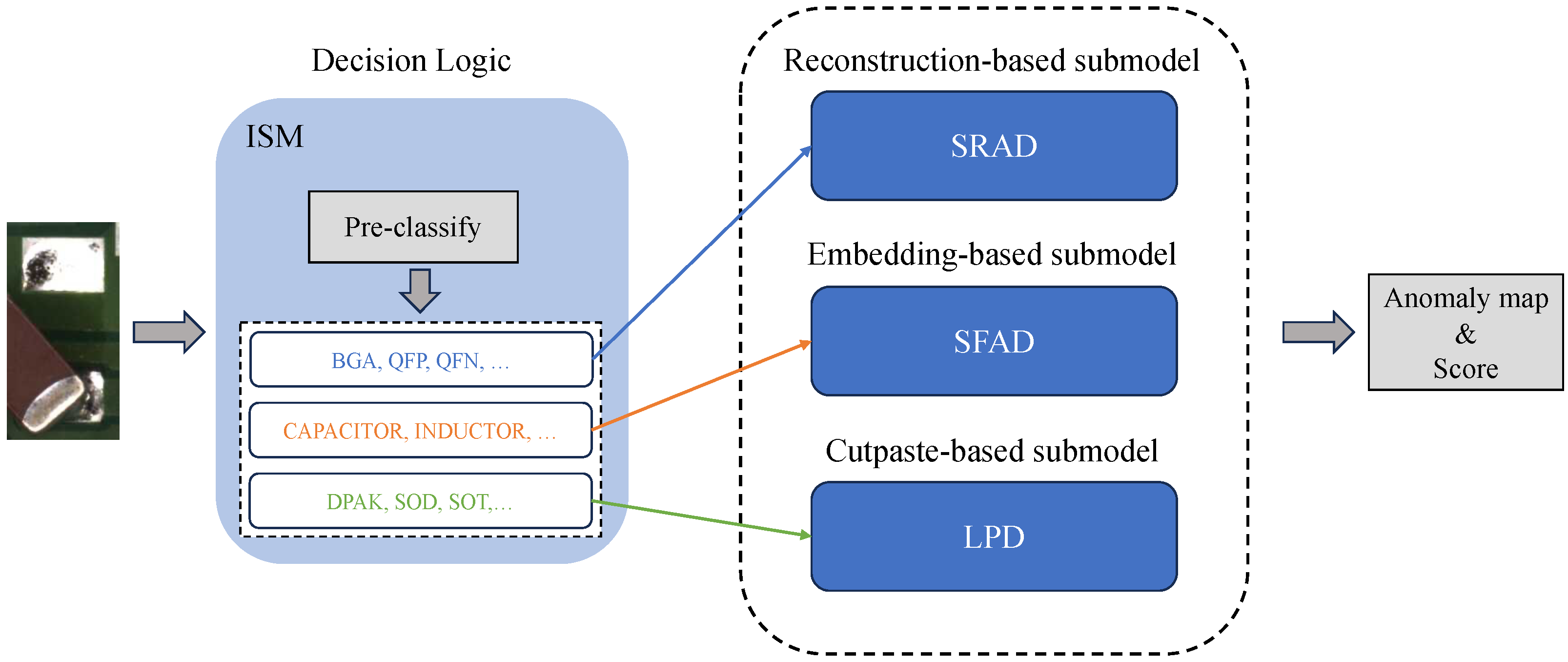
The overall architecture of MADE-Net is illustrated in Figure 1. It comprises three submodels and a dynamic integration and selection module. Specifically, SRAD, SFAD, and LPD correspond to the reconstruction-based, feature-based, and CutPaste-based approaches, respectively. In addition, we introduce a large-scale benchmark dataset, ManuDefect-21, which addresses the absence of negative samples in existing training sets. All proposed submodels are first trained in an unsupervised manner and subsequently fine-tuned on the entire training set of ManuDefect-21.

3.1. Reconstruction-Based Submodel

Reconstruction-based methods are among the most commonly used in the anomaly detection area. These methods derive their anomaly detection efficacy from the core hypothesis that neural networks, when trained exclusively on normal data, exhibit limited reconstruction fidelity for anomalous regions. This inherent limitation enables anomaly identification through pixel-wise or feature-wise comparisons between the input and its reconstructed output.

In our paper, SRAD (Submodel of Reconstruction-based Anomaly Detection) is designed as a part of the integrated model to compensate for the shortcomings of other submodels. The architecture of SRAD is outlined in Figure 2. The input image is used to synthesize anomaly samples. The synthesized sample is encoded and reconstructed using the autoencoder architecture model, aiming to reconstruct the synthesized anomaly into normal. The anomaly detection module is a Unet-based architecture that locates anomalous regions by comparing the input and reconstructed one. To address the foreground–background imbalance inherent in defect segmentation, we adopt Focal Loss [29], which adaptively down-weights easy negatives and highlights challenging anomalous regions.

3.1.1. Anomaly Synthesis Module

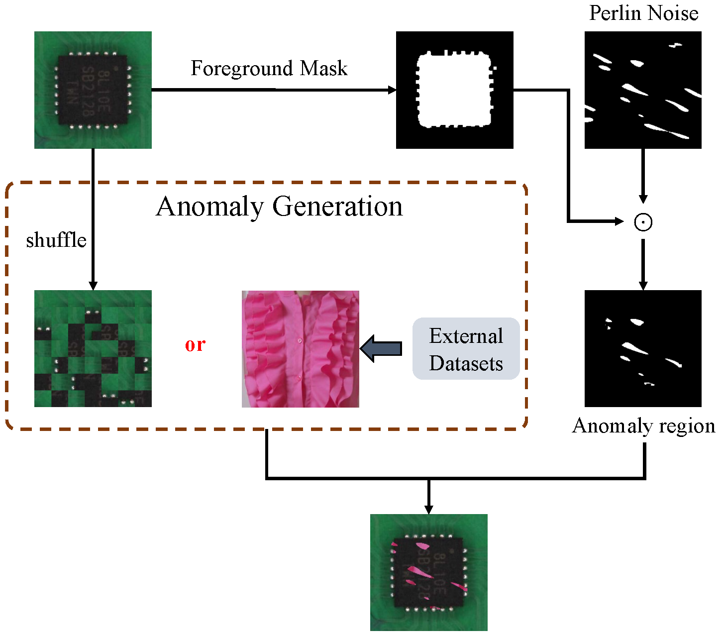
We adopt the anomaly generation strategy proposed in MSTUnet [30] to simulate both texture and structural anomalies. As illustrated in Figure 3, texture anomalies are generated by randomly selecting samples $I_{\mathrm{DTD}}$ from the DTD texture dataset [31], whereas structural anomalies are synthesized by shuffling and recombining patches extracted from a normal ground truth sample $N_{\mathrm{GT}}$. The resulting simulated anomaly is denoted as $\delta$.

An anomaly mask, ${\mathrm{mask}}_{\mathrm{ano}}$, is obtained via element-wise multiplication of a Perlin noise-based mask ${\mathrm{mask}}_p$ and a foreground mask ${\mathrm{mask}}_{\mathrm{fg}}$, where the latter is derived from the ground truth foreground region of $N_{\mathrm{GT}}$. This ensures that the injected anomalies are constrained to the primary object within the normal sample.

The final synthetic anomaly image is computed as

$$A_{\mathrm{Synth}}={\mathrm{mask}}_{\mathrm{ano}}\odot \delta +(1-{\mathrm{mask}}_{\mathrm{ano}})\odot N_{\mathrm{GT}},$$

(1)

where ⊙ denotes element-wise multiplication.

During training, texture and structural anomalies are introduced with equal probability to ensure balanced exposure to both anomaly types.

3.1.2. Reconstruction Module

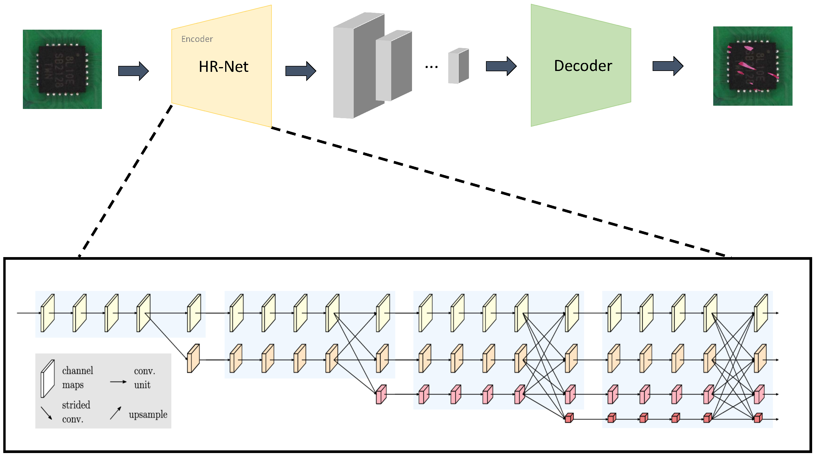
Since the synthesized anomalous sample and the corresponding anomalous mask are obtained, we propose a novel autoencoder-based reconstruction module. The architecture of the reconstruction module is shown in Figure 4.

Encoder

Current deep networks for feature encoding suffer from two critical limitations: (1) progressive resolution degradation, leading to the compromised representation of small anomalous features, and (2) insufficient multi-scale feature integration, resulting in suboptimal anomaly localization accuracy. To address these challenges, we employ HRNet-W32 [32] as the encoder backbone of our autoencoder-based reconstruction module, leveraging its unique parallel multi-resolution preservation architecture and dynamic feature exchange mechanism. The HRNet backbone preserves high-resolution feature representations throughout the reconstruction process, significantly improving the localization of small-scale defects. This design effectively maintains fine-grained anomaly signatures while simultaneously enhancing discriminative capability across diverse anomaly scales.

The input image $I\in {\mathbb{R}}^{H\times W\times 3}$ is initially processed through two stride-2 3 × 3 convolutional layers, generating a high-resolution feature map $F_1^{\left(1\right)}\in {\mathbb{R}}^{{\displaystyle \frac{H}{4}}\times {\displaystyle \frac{W}{4}}\times C}$ while maintaining 1/4 spatial resolution of the original input. The architecture progressively integrates multi-scale subnetworks across s stages ($s\in \{1,2,3,4\}$), where each subsequent stage incorporates additional parallel branches with geometrically decreasing resolutions ${\displaystyle \frac{H}{2^{s+1}}}\times {\displaystyle \frac{W}{2^{s+1}}}$ and exponentially increasing channel dimensions $C\times 2^{s-1}$. For instance, Stage 2 comprises dual parallel pathways: $F_1^{\left(2\right)}$ preserving the original 1/4 resolution and $F_2^{\left(2\right)}$ operating at 1/8 resolution.

Cross-resolution feature integration is achieved through adaptive transformation operators ${\varphi }_{i\to k}$ in the fusion function:

$$F_k^{\left(s\right)}=\sum _{i=1}^n{\varphi }_{i\to k}\left(F_i^{(s-1)}\right)$$

(2)

where the transformation mechanism adaptively applies

-

Upsampling ($i>k$): Bilinear interpolation followed by 1 × 1 convolution for channel alignment;

-

Downsampling ($i<k$): Strided-2 3 × 3 convolution with feature compression;

-

Identity mapping ($i=k$): Direct feature propagation.

The final feature encoding $\widehat{F}$ is synthesized through the channel-wise concatenation ${⨁}_{k=1}^4{F}_k^{\left(4\right)}$ of all subnetwork outputs, followed by spatial upsampling to match the original input dimensions. This architecture effectively preserves high-resolution representations throughout the network via persistent skip connections in the primary pathway, significantly enhancing the spatial localization accuracy for small-scale anomaly detection tasks.

Decoder

The decoder architecture processes the encoded feature representation $\widehat{F}$ through a hierarchical refinement pipeline comprising two sequential Residual Network (ResNet) blocks followed by two transposed convolutional upsampling modules. Each ResNet block integrates identity shortcut connections and consists of (1) a 3 × 3 convolutional layer with stride 1, (2) batch normalization, and (3) ReLU activation, designed to enhance feature expressiveness while mitigating gradient vanishing issues. The subsequent transposed convolution blocks progressively restore spatial resolution using 4 × 4 kernels with stride 2 and padding 1, systematically doubling the feature map dimensions at each stage through learnable upsampling operations. This dual-stage upsampling mechanism, interleaved with channel-wise feature recombination, transforms the latent representation into the reconstructed output image $I_{gen}\in {\mathbb{R}}^{H\times W\times 3}$ while preserving structural coherence.

3.1.3. Anomaly Detection Module

The purpose of the anomaly detection module is to localize the anomaly by inspecting the input image $N_{GT}$ and reconstructed image $I_{gen}$. The images are concatenated depth-wise and decoded into a segmentation mask M by a U-net-based architecture. M is the output anomaly map indicating the pixel-level location of the anomalies in the image. To also compute the image-level anomaly score, we apply a simple segmentation mask interpretation procedure—the segmentation mask is smoothed by a 21 × 21 averaging filter and globally max-pooled into a single score.

3.1.4. Loss Function and Inference

The reconstruction module aims at turning the anomalous sample into normal, and the Anomaly Detection Module is designed to locate the anomaly area. Since the anomaly is synthesized by the AS Module during the training stage, the ground truth anomaly mask is known. The loss function is defined below:

$${\mathcal{L}}_{\mathrm{total}}={\lambda }_{\mathrm{rec}}·{\mathcal{L}}_{\mathrm{rec}}(I_{\mathrm{gen}},N_{\mathrm{GT}})+{\lambda }_{\mathrm{seg}}·{\mathcal{L}}_{\mathrm{seg}}({\mathrm{mask}}_{\mathrm{ano}},M)$$

(3)

$${\mathcal{L}}_{\mathrm{rec}}={\displaystyle \frac{1}{HW}}\sum _{i=1}^H\sum _{j=1}^W{\left(I_{\mathrm{gen}}^{(i,j)}-N_{\mathrm{GT}}^{(i,j)}\right)}^2$$

(4)

$${\mathcal{L}}_{\mathrm{seg}}=-{\displaystyle \frac{1}{HW}}\sum _{i=1}^H\sum _{j=1}^W\left\{\begin{array}{cc}\alpha ·{(1-M_{ij})}^{\gamma }·log\left(M_{ij}\right),\hfill & \mathrm{if}{\left({\mathrm{mask}}_{\mathrm{ano}}\right)}_{ij}=1\hfill \\ (1-\alpha )·M_{ij}^{\gamma }·log(1-M_{ij}),\hfill & \mathrm{if}{\left({\mathrm{mask}}_{\mathrm{ano}}\right)}_{ij}=0\hfill \end{array}\right.$$

(5)

${\mathcal{L}}_{\mathrm{rec}}$ and ${\mathcal{L}}_{\mathrm{seg}}$ denote the reconstruction loss and segmentation loss, respectively. $I_{\mathrm{gen}}$ and $N_{\mathrm{GT}}$ represent the reconstructed image and the ground truth normal image. $\mathrm{mask}\mathrm{ano}$ and M are the binary ground truth mask of anomalous regions and the predicted anomaly mask. $\lambda \mathrm{rec}$ and ${\lambda }_{\mathrm{seg}}$ are hyperparameters used to balance the contributions of the reconstruction and segmentation losses. $\alpha$ and $\gamma$ are the focusing parameters of the Focal Loss, where $\alpha$ balances the importance of positive and negative examples, and $\gamma$ adjusts the rate at which easy examples are down-weighted.

3.2. Feature-Based Submodel

Feature-embedding-based methods represent a prominent class of approaches in image anomaly detection. These methods operate under the central assumption that neural networks trained solely on normal samples learn feature representations that are highly compact for normal data but exhibit significant deviations for anomalous inputs [8,22,33]. By mapping images into a latent feature space, anomalies can be identified by measuring the distance or similarity between an input’s embedded features and a reference distribution of normal features. This strategy enables effective anomaly detection by leveraging the discriminative power of learned feature embeddings.

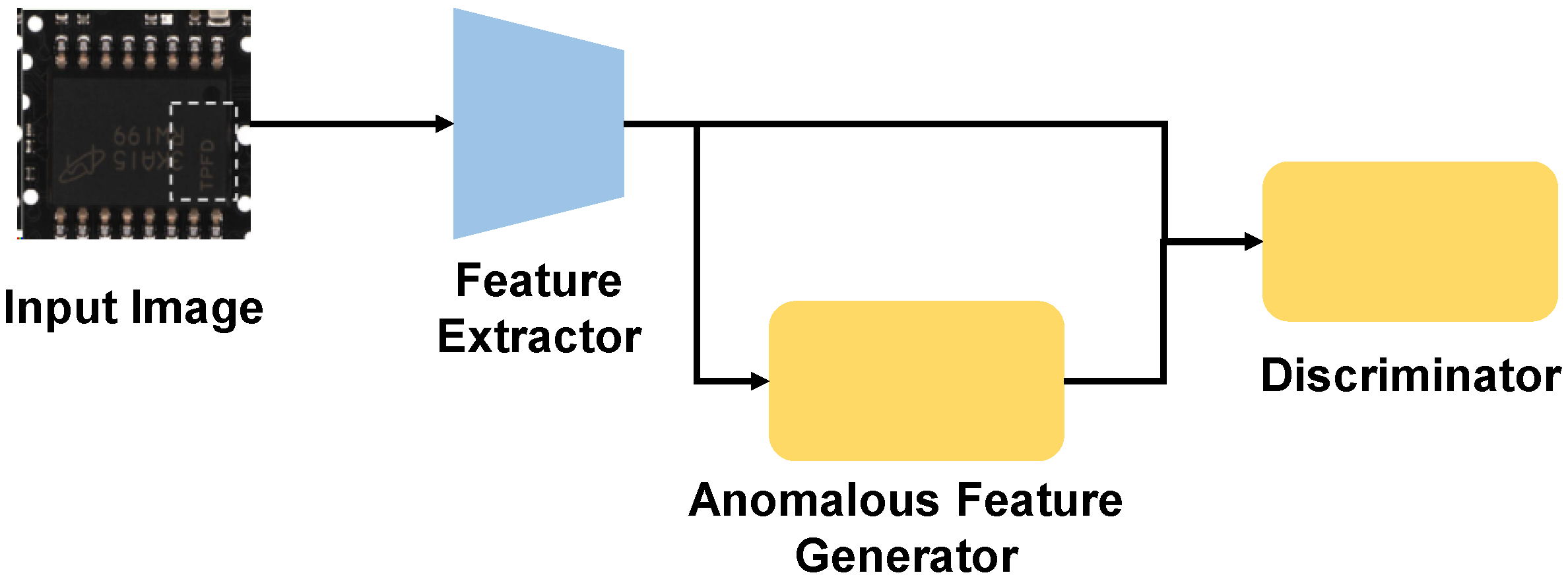
This subsection presents a comprehensive overview of SFAD (Submodel of Feature-based Anomaly Detection), a key part of our integrated model. SFAD integrates three essential components—a Feature Extractor, an Anomalous Feature Generator, and Discriminator—as illustrated in Figure 5.

During the training phase, an input image is passed through the Feature Extractor to yield a normal feature representation. Subsequently, the Anomalous Feature Generator takes this normal feature to create a synthetic anomalous counterpart. Both the normal and anomalous features are then fed to the Discriminator, which learns to differentiate them. For inference, the pipeline is simplified: the Anomalous Feature Generator is omitted, and the Feature Extractor passes its output directly to the Discriminator to produce the final anomaly score. The following subsections will examine each of these components in detail.

3.2.1. Feature Extractor

To capture semantic irregularities, we propose a feature extractor that exploits local contextual cues and hierarchical semantics. Given an input image $I_m\in {\mathbb{R}}^{H\times W\times 3}$ from the training set ${\mathcal{X}}_{\mathrm{train}}$ or the test set ${\mathcal{X}}_{\mathrm{test}}$, we apply a pretrained backbone network $\mathsf{\Phi }$ to extract intermediate feature maps from multiple layers.

To capture subtle anomalies, we design a feature representation module that leverages both local context and multi-level semantic information. Given an input image $I_m\in {\mathbb{R}}^{H\times W\times 3}$ from either the training set ${\mathcal{X}}_{\mathrm{train}}$ or the test set ${\mathcal{X}}_{\mathrm{test}}$, we first extract intermediate features from a pretrained backbone network $\mathsf{\Phi }$.

Since generic backbones pretrained on datasets like ImageNet may encode patterns irrelevant to industrial anomalies, we selectively retain a subset of layers L. This choice is a trade-off: deeper layers provide rich semantic information but have poor spatial resolution, while shallower layers offer finer detail but lack high-level context. Our selection is empirically driven to balance these factors, a common practice in feature-based methods. Each chosen feature map is represented as ${\varphi }^{l,i}={\varphi }^l\left(x_i\right)\in {\mathbb{R}}^{H_l\times W_l\times C_l}$, where $l\in L$.

To incorporate spatial locality, which is crucial for distinguishing local texture from anomalous defects, we define a neighborhood window of size $p\times p$ around each spatial position $(h,w)$:

$$\begin{array}{cc}\hfill {\mathcal{N}}_p^{(h,w)}=\{(h^{\prime },w^{\prime })\mid h^{\prime }& \in [h-\lfloor p/2\rfloor ,h+\lfloor p/2\rfloor ],\hfill \\ \hfill w^{\prime }& \in [w-\lfloor p/2\rfloor ,w+\lfloor p/2\rfloor ]\}.\hfill \end{array}$$

(6)

A local aggregation operation is then applied over each neighborhood to produce a context-aware descriptor:

$$z_{h,w}^{l,i}=f_{\mathrm{agg}}(\{{\varphi }_{h^{\prime },w^{\prime }}^{l,i}\mid (h^{\prime },w^{\prime })\in {\mathcal{N}}_p^{(h,w)}\}).$$

(7)

All aggregated feature maps $z^{l,i}$ are subsequently rescaled to a common spatial resolution $(H_0,W_0)$, typically matching the largest map, and concatenated along the channel dimension to form a unified representation.

We denote the resulting local feature at spatial location $(h,w)$ as $o_{h,w}^i\in {\mathbb{R}}^C$.

To bridge the domain gap between generic pretrained features and task-specific industrial features, a lightweight embedding transformation $G_{\theta }$ is applied. This module, typically a shallow CNN, adapts the generic local feature $o_{h,w}^i$ to a task-specific embedding $q_{h,w}^i\in {\mathbb{R}}^{C^{\prime }}$ without adding significant computational complexity:

$$q_{h,w}^i=G_{\theta }\left(o_{h,w}^i\right).$$

(8)

For brevity, the complete feature extraction and transformation process can be represented as a single function:

$$q^i=F_{\varphi ,\theta }\left(x^i\right),$$

(9)

where $F_{\varphi ,\theta }$ encapsulates both multi-level feature extraction via $\mathsf{\Phi }$ and subsequent task-specific adaptation via $G_{\theta }$.

3.2.2. Anomalous Feature Generator

Effective training of a discriminative anomaly detection model requires not only representative normal samples but also suitable negative examples to define clear decision boundaries. Obtaining real defective samples is often difficult. While prior studies [25,26,34] often rely on complex image-space augmentations to generate pseudo-anomalies, these can introduce unrealistic artifacts or have an unpredictable effect on feature representations. Here, we adopt a more direct and controlled approach by perturbing features in the latent space. This allows us to explicitly simulate the effect of an anomaly—a deviation from the normal feature manifold—rather than its visual appearance.

Specifically, let $q_{h,w}^i\in {\mathbb{R}}^C$ denote a local feature vector. We synthesize its negative counterpart by adding random noise $ϵ$ from an isotropic Gaussian distribution:

$$q_{h,w}^{i-}=q_{h,w}^i+ϵ,ϵ\sim \mathcal{N}(\mu ,{\sigma }^{2}I),$$

(10)

where each dimension of $ϵ$ is independently drawn. This isotropic perturbation ensures that we do not make strong assumptions about the nature of anomalies, making the model sensitive to a wide variety of deviations.

This method’s strength lies in its simplicity and directness, providing clear negative examples for training the discriminator. However, we acknowledge its limitation: the synthetic features are not guaranteed to correspond to the representations of real-world defects and lack semantic meaning. The goal is not to perfectly mimic real anomalies, but to effectively train the discriminator to learn a tight decision boundary around the normal data manifold, thereby making it sensitive to any feature that falls “off-manifold”.

3.2.3. Discriminator

We design a Discriminator $D_{\psi }$ to estimate a normality score at each spatial location $(h,w)$. The discriminator must distinguish on-manifold (normal) features from off-manifold (perturbed) ones. For this task, a simple Multi-Layer Perceptron (MLP) is sufficient and computationally efficient, as it operates on individual feature vectors. This avoids the complexity and potential for overfitting that a larger model might introduce. The discriminator is encouraged to output high scores for normal features and low scores for perturbed ones.

3.2.4. Training Objective and Optimization Strategy

To enable the model to differentiate between normal and perturbed features, we employ a margin-based objective inspired by truncated regression losses. Specifically, for each spatial location $(h,w)$ in the feature map, we compute a sample-wise loss as

$${\ell }_{h,w}^i=max(0,{\tau }^{+}-D_{\psi }\left(q_{h,w}^i\right))+max(0,D_{\psi }\left(q_{h,w}^{i-}\right)-{\tau }^{-}),$$

(11)

where $D_{\psi }$ is a discriminative scoring function parameterized by $\psi$, applied to both clean features $q_{h,w}^i$ and their corrupted counterparts $q_{h,w}^{i-}$. $\tau$ is the margin controlling the confidence window, set to 0.5 in our experiments.

The total objective over the training dataset ${\mathcal{X}}_{\mathrm{train}}$ is given by

$$\mathcal{L}(\theta ,\psi )=\sum _{x^i\in {\mathcal{X}}_{\mathrm{train}}}\sum _{h,w}{\displaystyle \frac{{\ell }_{h,w}^i}{H_0·W_0}},$$

(12)

where $\theta$ denotes parameters of the feature adaptor, and optimization is performed jointly over $\theta$ and $\psi$. This formulation encourages the Discriminator to assign high scores to normal regions while penalizing confidently misclassified anomalies beyond a predefined confidence band.

3.2.5. Inference and Anomaly Scoring

During inference, the synthetic anomaly generator is removed, resulting in a fully differentiable end-to-end architecture consisting solely of the feature extractor $F_{\varphi ,\theta }$ and the discriminator $D_{\psi }$. For a given test image $x_i\in {\mathcal{X}}_{\mathrm{test}}$, the adapted feature map is computed as

$$q^i=F_{\varphi ,\theta }\left(x_i\right),$$

(13)

where $q_{h,w}^i$ denotes the feature descriptor at spatial location $(h,w)$.

Anomaly scores are assigned to each spatial position using the learned discriminator:

$$s_{h,w}^i=-D_{\psi }\left(q_{h,w}^i\right),$$

(14)

with higher values corresponding to a higher likelihood of abnormality.

To obtain a spatially resolved representation of potential anomalies, we construct the anomaly map.

$$S_{\mathrm{loc}}\left(x_i\right)=\{s_{h,w}^i\mid (h,w)\in [1,H_0]\times [1,W_0]\}.$$

(15)

this map is upsampled to the original image resolution using bilinear interpolation and further smoothed with a Gaussian filter ($\sigma =4$) to suppress boundary noise and enhance spatial coherence.

For image-level anomaly detection, a single scalar score is derived by taking the maximum over all spatial positions:

$$S_{\mathrm{img}}\left(x_i\right)=\underset{(h,w)\in [1,H_0]\times [1,W_0]}{max}{s}_{h,w}^i.$$

(16)

This strategy ensures that even small but pronounced anomalous regions contribute strongly to the final decision, making the framework sensitive to subtle defects irrespective of their spatial extent.

3.3. Localized Patch Discrimination

In industrial images, normal samples typically exhibit high local structural consistency, meaning that local regions maintain natural continuity with their surrounding context in terms of texture, edges, and color. Based on this assumption, cutting and pasting a local region of an image to a different location disrupts the original structural consistency, thereby creating a localized perturbation that simulates a potential anomaly. Although such perturbations are not real defects, they effectively introduce local structural inconsistencies that can serve as training signals to guide the model in learning to recognize anomalies.

Based on this principle, this paper proposes the Localized Patch Discrimination (LPD). Unlike prior CutPaste-style methods, LPD defines standardized criteria for patch size and perceptibility, integrates self-supervised training directly into the MADE-Net framework, and leverages the learned anomaly-sensitive features for downstream detection tasks, thereby providing both a principled perturbation mechanism and transferable representations. LPD employs a self-supervised learning mechanism. Specifically, it first constructs perturbed images from normal samples by cutting and pasting patches within the same image to generate “pseudo-anomalies”. Then, a discriminative model is trained to distinguish between the original normal images and the perturbed ones, thereby encouraging the model to focus on fine-grained differences in local structures. As shown in the Figure 6, the overall architecture of LPD is presented.

3.3.1. Local Patch Distortion Generation

Given a normal image $I\in {\mathbb{R}}^{H\times W\times 3}$, we generate an anomalous counterpart $\tilde{I}$ by cutting a rectangular patch $P\subset I$ and pasting it into a different location in the same image. The patch size is a crucial hyperparameter and is selected as a fraction of the image size to ensure that the perturbation is sufficiently localized yet perceptible enough to be learned by the model. During training, both the cut patch position and the target paste location are randomly sampled to increase the diversity of synthetic anomalies. Additionally, geometric transformations such as rotation and flipping may be applied to the patch before pasting to simulate a wider range of possible defects.

In this study, the “perceptibility” of a patch is defined and assessed through two complementary criteria: (1) a size standard based on relative area and (2) a perceptibility evaluation grounded in statistical differences. Specifically, the patch size is set as a fixed proportion of the original image area (typically 5–20%), determined through preliminary and ablation experiments to ensure that the patch is neither too small to be captured by the model nor so large that it disrupts the global semantics.

To evaluate perceptibility, we employ two measures. First, we compute quantitative differences between the patched region and its surrounding context in terms of texture, color, and structural similarity (e.g., SSIM, mean squared error, edge intensity). Second, we conduct sampled human inspection to confirm that the perturbation is visually discernible.

This standardized procedure ensures that the patch perturbations remain stable across samples and sufficiently localized to be effectively learned and recognized by the model, thereby providing a consistent training signal for anomaly detection.

This procedure creates a realistic and diverse set of localized anomalies that mimic common industrial defects characterized by local disruption of texture or structure. Unlike global image transformations, such as color jitter or blurring, patch recomposition preserves the overall global semantics while introducing subtle but detectable local inconsistencies.

3.3.2. Self-Supervised Learning Objective

The LPD module employs a convolutional neural network (CNN) backbone—typically a ResNet variant—to extract hierarchical feature representations from input images. We adopt ResNet as the backbone due to its proven ability to learn rich and stable feature hierarchies, residual connections that alleviate vanishing gradients, and its effectiveness in a wide range of industrial inspection tasks. Compared with deeper or more complex architectures (e.g., Vision Transformers), ResNet strikes a balance between representational power and computational efficiency, making it well-suited for large-scale industrial datasets.

The extracted features are then fed into a lightweight classification head consisting of fully connected layers that output the probability $p_{\theta }\left(x\right)$ of the input image x being anomalous. Since our task is essentially a binary discrimination between normal and patched (“pseudo-anomalous”) images, we adopt the binary cross-entropy (BCE) loss. BCE directly models the Bernoulli likelihood for two-class classification, provides well-calibrated probabilistic outputs, and is simpler and more stable than alternatives such as focal loss when the positive and negative classes are reasonably balanced.

We define a binary classification task where normal images are labeled as $y=0$ and patched images as $y=1$. The model is trained using the binary cross-entropy loss:

$${\mathcal{L}}_{PRP}=-{\mathbb{E}}_{(x,y)}\left[ylog{p}_{\theta }\left(x\right)+(1-y)log(1-p_{\theta }\left(x\right))\right]$$

(17)

minimizing this loss encourages the model to learn discriminative features that highlight localized inconsistencies introduced by patch recomposition.

To further enhance the quality of the feature, regularization techniques such as dropout and batch normalization are applied during training. Data enhancement strategies—including patch recomposition—are also used in normal images to improve the robustness of the model.

3.3.3. Feature Transfer and Ensemble Integration

After the self-supervised training phase, the classification head is discarded and the CNN backbone serves as a pretrained feature extractor. The learned representations effectively capture localized anomalies, which can be leveraged in downstream tasks such as object detection and the classification of electronic components.

Specifically, the pretrained backbone weights initialize the feature extractor in a supervised target detection framework (e.g., Faster R-CNN [35]), providing a strong initialization that accelerates convergence and improves final detection performance. Alternatively, features of LPD can be fused as auxiliary inputs alongside conventional features, enriching the representation with anomaly-sensitive cues.

3.4. Integration and Selection Module

The Integration and Selection Module (ISM) serves as a key component in MADE-Net, enabling dynamic model selection according to the characteristics of each input image. Rather than applying a uniform model to all data, ISM performs a two-stage procedure: (1) pre-classifying the input into 1 of 11 predefined component subcategories, and (2) selecting the most suitable anomaly detection submodel for that category based on empirical performance.

Stage 1: Pre-classification. We employ an EfficientNet-B4 network as the classifier due to its favorable trade-off between accuracy and computational cost in industrial settings. The classifier takes RGB images as input and outputs probabilities across 11 component types (e.g., BGA, CAPACITOR, RESISTOR). It is pretrained on ImageNet and fine-tuned on the ManuDefect-21 training set. The final class prediction $\widehat{y}$ is obtained by $\widehat{y}=argmax\left(p_i\right)$, where $p_i$ denotes the softmax probability for category i. Only predictions with confidence above 0.85 are accepted; otherwise, the default submodel (SFAD) is invoked to ensure stability. This mechanism enhances robustness against potential misclassification.

Stage 2: Model selection via performance map. A performance map M is constructed based on the results of extensive ablation studies. For each category c, we compute the average AUROC and Pixel-AP achieved by each submodel $\{S_{SRAD},S_{SFAD},S_{LPD}\}$ on its validation subset. The optimal model $S_c^{\ast }$ is determined by

$$S_c^{\ast }=arg\underset{S}{max}[\alpha ·\mathrm{AUROC}(S,c)+(1-\alpha )·\mathrm{PixelAP}(S,c)],$$

where $\alpha =0.5$ balances image- and pixel-level accuracy. The resulting mapping $M=\left\{(c,S_c^{\ast })\right\}$ is stored and used during inference. This data-driven assignment ensures that each subcategory is processed by the submodel best suited to its typical defect morphology.

3.5. Full-Supervised Fine-Tuning

For all three submodels, we adopt a two-stage training strategy consisting of initial unsupervised training followed by full-supervised fine-tuning. In the unsupervised stage, only normal samples from the training set are utilized. Synthetic anomalies are randomly generated and injected into normal images, and the models are trained to segment and localize these artificial anomalies. This allows the networks to learn robust representations of normal patterns and their structural consistency.

Benefiting from the availability of accurately annotated samples in our dataset, which provides both normal and anomalous instances in the training and test sets, we further introduce a supervised fine-tuning stage. After the unsupervised pretraining, all submodels are fine-tuned using the entire training set that includes both positive and negative samples along with pixel-level annotations. Unlike prior work where supervised refinement is limited by the absence of defect annotations, our dataset enables the direct replacement of synthetic anomalies with real anomalies and their masks during fine-tuning. This transition allows the models to adapt from artificially constructed defects to authentic defect distributions, bridging the gap between simulation and reality. While this strategy demonstrates clear benefits in improving discriminative power under well-annotated conditions, we acknowledge that its applicability in scenarios without exhaustive annotations remains limited. Nevertheless, we consider our approach a step toward bridging unsupervised pretraining and real-world supervised adaptation in industrial anomaly detection.

This two-stage paradigm preserves the generalization capability of unsupervised training while fully exploiting the availability of labeled data, leading to improved accuracy and practical applicability in industrial scenarios.

3.6. Dataset ManuDefect-21

We proposed ManuDefect-21, a specialized dataset sampled from a real-world SMT (surface mount technology) industrial production line. As demonstrated in

Table 2. Dataset comparison across different industrial inspection benchmarks.

Dataset	#Train	#Test (Good)	#Test (Anomaly)	#Defect Classes
MVTec AD [11]	3629	467	1258	73
VisA [12]	8659	962	1200	78
ManuDefect-21	31,050	10,272	3049	82

, our proposed dataset exhibits substantial advantages in terms of scale and diversity compared to existing benchmarks. Specifically, our dataset contains 31,050 training images, which is approximately 8.6 times larger than MVTec AD [11] and 3.6 times larger than VisA [12]. ManuDefect-21’s test set comprises 10,272 normal samples and 3049 anomalous samples, providing a more comprehensive evaluation platform with balanced representation of both normal and defective cases. Furthermore, our dataset encompasses 82 distinct defect types, surpassing the variety of defect types covered in both MVTec AD (73 types) and VisA (78 types). This extensive collection of diverse defect patterns enables more robust evaluation of anomaly detection methods and better reflects the complexity of real-world industrial inspection scenarios.

Limitations and scope: While ManuDefect-21 offers significant scale and diversity, it also has limitations. Some subcategories, such as ALUMINUM_CAPACITOR, contain relatively few samples, which may affect the reliability of evaluation and model generalization for rare categories. Future work should consider expanding the dataset to cover more process types and address sample imbalance for rare categories.

Table 3. Detailed breakdown of ManuDefect-21 dataset subcategories.

Category	#Train	#Train (Good)	#Train (Anomaly)	#Test (Good)	#Test (Anomaly)	#Defect Types
ALUMINUM_CAPACITOR	505	496	9	214	4	5
BGA	794	611	183	262	79	6
CAPACITOR	9945	7007	2938	3004	1260	7
DPAK	771	517	254	222	110	8
INDUCTOR	3502	3485	17	1494	8	5
QFN	1441	1155	286	495	123	9
QFP	4680	4138	542	1774	233	10
RESISTOR	2162	890	1272	382	546	8
SOD	2037	1105	932	474	400	8
SOIC	4288	3285	463	1640	199	9
SOT	925	724	201	311	87	7
Total	31,050	23,953	7097	10,272	3049	82
Mean	2823	2178	645	934	277	8
Ratio	-	3.375	1	3.369	1	-

provides a detailed breakdown of our dataset across different electronic component categories, demonstrating the comprehensive coverage of various industrial inspection scenarios.

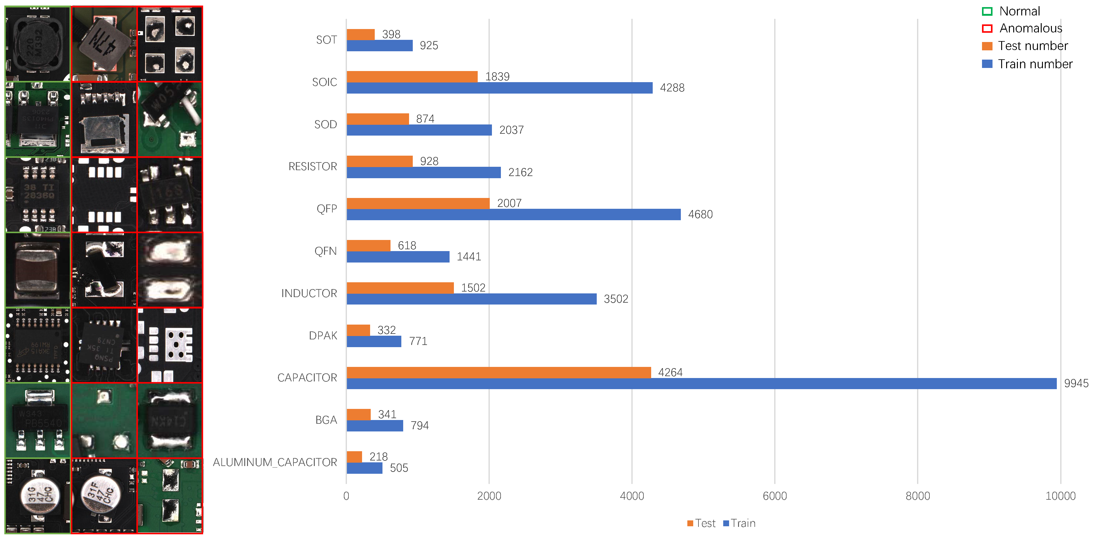
Our dataset covers 11 major electronic component categories commonly found in industrial manufacturing, including capacitors, resistors, inductors, and various integrated circuit packages (BGA, QFN, QFP, SOIC, SOT, SOD, DPAK). Each category contains a substantial number of training samples, with CAPACITOR being the largest category (9945 training images) and ALUMINUM_CAPACITOR being the smallest (505 training images). The dataset maintains a balanced distribution across different defect types, with an average of 8 anomaly types per category, ranging from 5 to 10 types per component category.

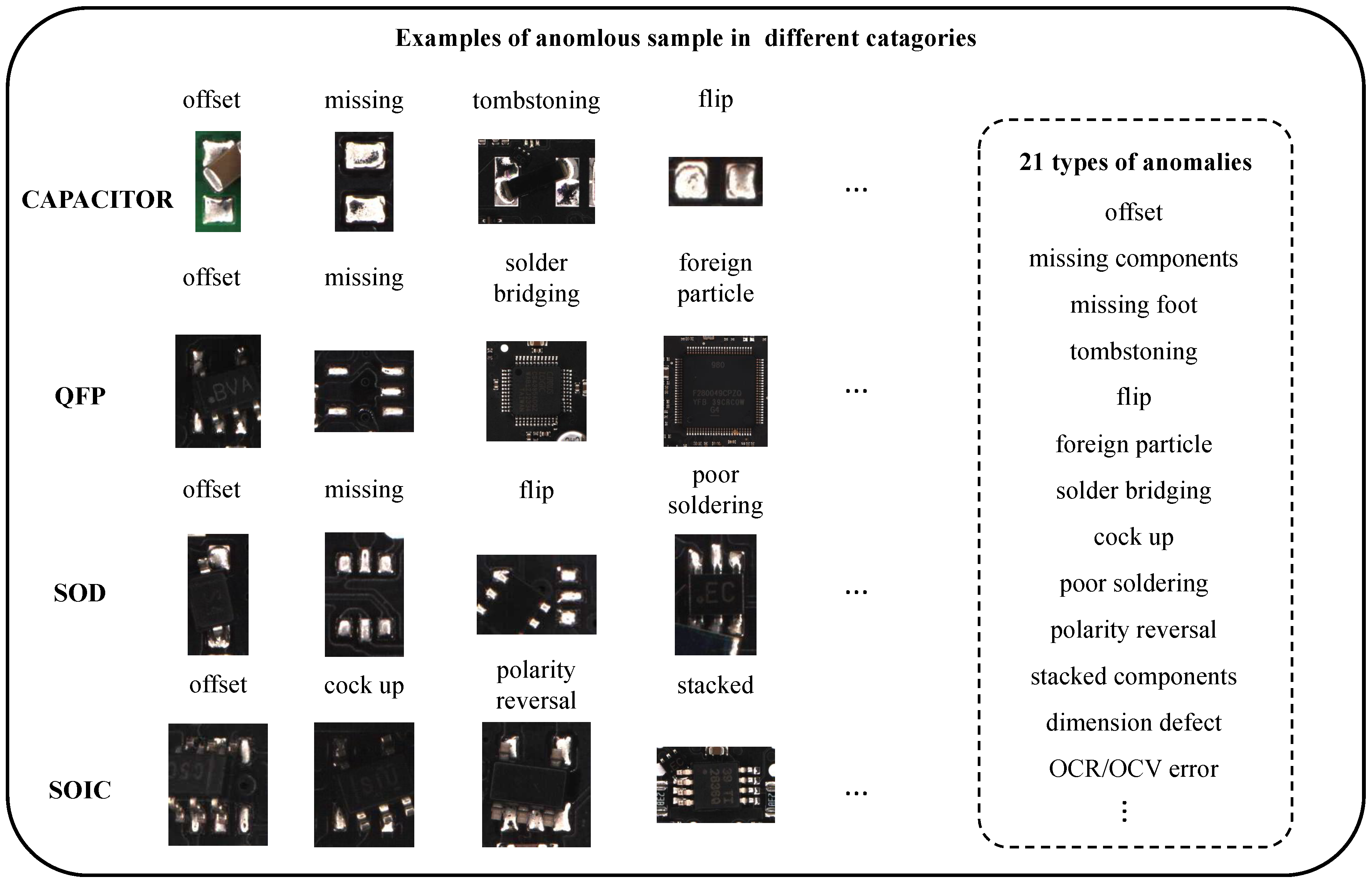
As Figure 7 shows, our dataset includes 21 well-defined anomaly types spanning mounting, soldering, and surface contamination defects, offering a comprehensive coverage of typical industrial production anomalies. Several anomaly categories exhibit subtle inter-class differences, making the dataset particularly suitable for fine-grained classification and robustness evaluation. In addition to diversity in defect types, the dataset also features challenging visual conditions, such as varying contrast, partial occlusion, and reflective interference, providing a realistic testbed for evaluating model generalization. Through detailed labeling of anomaly types, our dataset expands its applicability beyond image-level anomaly detection to include fine-grained classification of specific defect categories.

Anomaly taxonomy and distinction: For closely related defect types (e.g., insufficient solder vs. cold joint), we follow industrial inspection standards and expert annotation guidelines to define clear classification criteria. Insufficient solder is characterized by a visibly reduced solder volume, while cold joints are identified by dull, grainy surfaces and poor electrical connectivity. All anomaly types are annotated with reference to their physical characteristics and failure modes, ensuring that the dataset supports fine-grained and meaningful classification.

Figure 8 presents the sample distribution and representative images of 11 categories of electronic components in our dataset. The left panel shows images of typical categories, where green bounding boxes indicate normal samples and red bounding boxes denote anomalous samples of the corresponding category. Seven representative categories, including INDUCTOR, RESISTOR, and QFP, are selected to visually illustrate the appearance differences between normal and anomalous instances. The bar chart on the right summarizes the number of samples per category in the training and test sets. It can be observed that the data scale varies across categories, reflecting the actual occurrence frequency and defect probability of components in real production lines. For example, CAPACITOR contains 9945 and 4264 images in the training and test set, respectively, and it is a device with a relatively high occurrence frequency in the production line. The number of ALUMINUM_CAPACITOR images is relatively small, with 505 images in the training set and 218 images in the test set. This type of data distribution reflects that, in actual industrial scenarios, the failure rate of certain devices themselves is extremely low, making it difficult to collect sufficient abnormal samples. Despite this, this dataset still contains a sufficient number of samples in each category, and its overall scale is much larger than that of widely used anomaly detection datasets such as MVTec and VisA. Moreover, ManuDefect-21 provides both normal and anomalous samples in both the training and test sets, while preserving the real-world positive/negative sample ratio observed on production lines. This design not only better reflects the conditions of actual manufacturing environments but also offers a robust basis for evaluating the performance of anomaly detection methods in practical industrial applications.

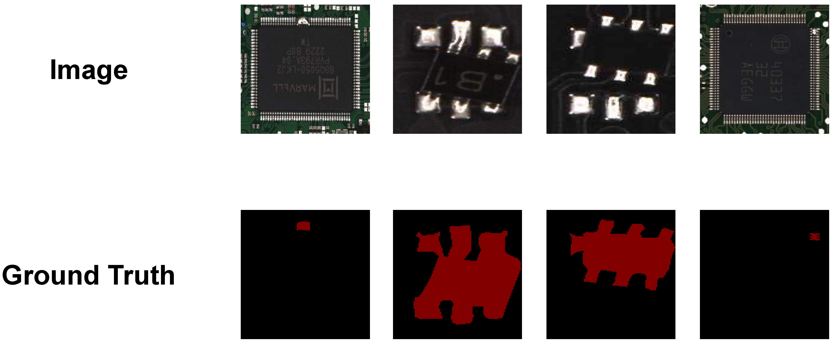
Additionally, a distinctive feature of the ManuDefect-21 dataset is the provision of fine-grained pixel-level annotations for training and evaluation phases, enabling precise anomaly localization and segmentation assessment across all stages of model development. As shown in Figure 9, these detailed annotations facilitate the comprehensive assessment of model performance in both image-level detection and pixel-level localization tasks, which is particularly valuable for industrial applications requiring precise defect identification and boundary delineation.

4. Experiments and Results

In this section, we present a comprehensive evaluation of the proposed MADE-Net framework on the newly introduced ManuDefect-21 dataset, which contains 31,050 training and 13,321 test images across 11 component categories and 82 distinct defect types, captured under real production conditions. Our evaluation is structured to assess model performance and component contributions. Specifically, we will (1) compare MADE-Net against state-of-the-art baseline methods (DSR, SimpleNet, CutPaste) using both image-level and pixel-level metrics, and (2) conduct a detailed ablation study to quantify the contribution of each submodel within our framework. This rigorous analysis demonstrates the effectiveness and practical advantages of our approach in complex industrial settings.

4.1. Experimental Setup

All experiments were conducted on an NVIDIA RTX 4090 GPU using PyTorch 2.1. We employed the Adam optimizer with an initial learning rate of 1 × ${10}^{-4}$, batch size of 8, and input resolution of 256 × 256, with early stopping applied after 10 consecutive epochs without validation improvement. These hyperparameters were determined through grid search on the validation split of the ManuDefect-21 dataset to balance convergence speed and generalization.

4.2. Baseline Methods

To contextualize the performance of our proposed MADE-Net, we benchmark it against three state-of-the-art (SOTA) anomaly detection methods: DSR, SimpleNet, and CutPaste. These baselines were selected because they represent distinct and influential paradigms in anomaly detection, each corresponding to a core principle integrated within our multi-branch MADE-Net framework. The comparison aims to demonstrate that our synergistic approach, which combines reconstruction-based, feature-based, and self-supervised learning principles, achieves superior and more robust performance than methods that rely on a single strategy. Specifically, we will highlight how MADE-Net overcomes the limitations of individual approaches by leveraging their complementary strengths.

DSR (Dual Subspace Re-projection Network) [3] is an unsupervised anomaly detection framework that leverages a dual-decoder architecture and quantized feature space. It operates by (1) extracting features using a pretrained backbone, (2) generating pseudo-anomalous features via latent space perturbation, and (3) training two decoders—one reconstructing normal samples, and the other reconstructing perturbed features. The model is optimized to minimize reconstruction error for normal data and maximize it for pseudo-anomalies, enabling the robust separation of normal and anomalous patterns. At inference, only the backbone and primary decoder are used for fast prediction. DSR’s effectiveness stems from its feature-space anomaly simulation and dual-branch design, supporting accurate detection and localization across diverse defect types.

SimpleNet [36] is a lightweight anomaly detection framework designed for ease of deployment. It employs (1) a pretrained backbone to extract local representations, (2) a compact adapter to align these representations with the target domain, (3) a feature perturbation module that fabricates pseudo-anomalous features via Gaussian noise injection, and (4) a binary discriminator separating altered from pristine features. At inference time, only the backbone, adapter, and discriminator are retained, yielding fast prediction. Its effectiveness stems from minimal architectural overhead combined with feature-space anomaly simulation, enabling competitive detection and localization quality.

CutPaste [25] is a self-supervised approach that learns discriminative features using only normal data by formulating a surrogate task: distinguishing untouched images from versions in which a patch has been cut out and pasted elsewhere (optionally resized or rotated). After this pretext training, a one-class generative classifier is fit on the learned embeddings. The simple patch relocation operation induces sensitivity to structural and textural irregularities, allowing the method to generalize to varied defect types and support coarse-to-fine localization through patch-level scoring.

4.3. Evaluation Metrics

For a comprehensive evaluation of anomaly detection performance, both image-level and pixel-level metrics are employed to assess detection accuracy and localization precision:

Metric selection and industrial relevance: We mainly adopt AUROC and AP as evaluation metrics, which are widely recognized for their ability to comprehensively reflect model performance and facilitate fair comparison. AUROC measures the overall discrimination ability between normal and anomalous samples, while AP summarizes precision–recall trade-offs. To provide a thorough assessment, we report both image-level and pixel-level results, capturing detection and localization performance, respectively.

Moreover, in real manufacturing environments, the cost of false positives (misidentifying normal regions as defective) and false negatives (missing critical defects) can be substantial. The chosen metrics help quantify overall detection and localization ability, but practitioners should also consider application-specific requirements, such as the impact of missing small but critical defects or the operational cost of excessive false alarms. We encourage future work to incorporate cost-sensitive and defect-size-aware metrics to better reflect practical needs.

Image-level Metrics

• AUC (Area Under the ROC Curve): This metric quantifies the model’s ability to differentiate between normal and anomalous images across all threshold values. A perfect classifier achieves an AUC of 1.0, while random classification results in an AUC of 0.5.
• AP (Average Precision): This metric computes the area under the precision–recall curve, offering insights into the model’s performance across varying recall levels, and is particularly valuable for imbalanced datasets.

Pixel-level Metrics

• Pixel-level AUC: This metric evaluates the model’s capacity to accurately localize anomalous regions within images, treating each pixel as a binary classification target (normal vs. anomalous).
• Pixel-level AP: This metric measures the precision of anomaly localization by calculating the average precision across different threshold values for pixel-wise anomaly scores.

These metrics provide a holistic assessment framework, where image-level metrics evaluate the overall detection performance, and pixel-level metrics assess the accuracy of anomaly localization and segmentation.

4.4. Performance

We evaluate the performance of our proposed MADE-Net framework on the ManuDefect-21 dataset by comparing it with state-of-the-art anomaly detection methods. To ensure fair and accurate comparison, we reimplemented all baseline methods from scratch using the same experimental setup and hyperparameter optimization procedures.

We present a detailed performance breakdown across the 11 subcategories of the ManuDefect-21 dataset in

Table 4. Detailed performance comparison (AUC/AP) by subcategory on the ManuDefect-21 dataset. The best results in each row are highlighted in bold.

Category	Image-Level AUC/AP				Pixel-Level AUC/AP
	SimpleNet	CutPaste	DSR	MADE-Net	SimpleNet	CutPaste	DSR	MADE-Net
ALUMINUM_CAPACITOR	0.985/0.942	0.989/0.951	0.991/0.958	0.995/0.963	0.960/0.682	0.968/0.695	0.971/0.701	0.982/0.715
BGA	0.952/0.891	0.961/0.903	0.972/0.921	0.970/0.918	0.921/0.601	0.935/0.623	0.952/0.654	0.949/0.648
CAPACITOR	0.961/0.912	0.970/0.927	0.978/0.939	0.990/0.958	0.935/0.634	0.951/0.658	0.960/0.672	0.975/0.695
DPAK	0.970/0.931	0.978/0.944	0.984/0.953	0.983/0.951	0.945/0.652	0.963/0.680	0.959/0.674	0.960/0.675
INDUCTOR	0.975/0.948	0.983/0.959	0.981/0.954	0.982/0.955	0.950/0.661	0.965/0.684	0.973/0.699	0.971/0.692
QFN	0.965/0.924	0.972/0.936	0.979/0.945	0.991/0.962	0.938/0.639	0.955/0.662	0.965/0.681	0.964/0.678
QFP	0.968/0.929	0.975/0.941	0.983/0.952	0.981/0.950	0.942/0.646	0.958/0.669	0.966/0.683	0.979/0.707
RESISTOR	0.958/0.915	0.965/0.927	0.975/0.939	0.989/0.960	0.928/0.622	0.945/0.645	0.957/0.663	0.954/0.661
SOD	0.972/0.938	0.980/0.950	0.985/0.958	0.994/0.972	0.948/0.654	0.962/0.677	0.970/0.689	0.981/0.712
SOIC	0.963/0.921	0.974/0.936	0.971/0.932	0.972/0.934	0.936/0.637	0.956/0.668	0.952/0.661	0.953/0.663
SOT	0.970/0.934	0.977/0.946	0.983/0.954	0.993/0.968	0.946/0.650	0.961/0.673	0.969/0.685	0.980/0.708
Mean	0.967/0.926	0.975/0.938	0.980/0.946	0.985/0.954	0.941/0.643	0.956/0.667	0.963/0.678	0.968/0.687

. This table compares the image-level and pixel-level AUC scores of MADE-Net with the baseline methods for each component type.

From Table 4, it can be observed that the proposed two-stage model MADE-Net achieves the best overall performance. At both the image-level and pixel-level, MADE-Net consistently outperforms the baselines in terms of average AUC and AP (image-level: 0.985/0.954; pixel-level: 0.968/0.687), demonstrating its strong capability in anomaly detection and localization.

However, a more detailed analysis reveals that, while MADE-Net excels on average, its performance is not uniformly dominant across all categories. For instance, in categories like BGA, DPAK, and SOIC, baseline methods such as DSR and CutPaste achieve comparable or even superior results on certain metrics. This suggests that the optimal anomaly detection strategy may be category-dependent. The structural complexity and defect characteristics of components like BGA or SOIC might be better captured by the specialized mechanisms of single-paradigm models.

While MADE-Net demonstrates strong overall performance, it also has potential limitations. The model’s computational complexity is higher than single-branch baselines, and its reliance on synthetic anomalies may lead to overfitting or reduced generalization to real-world defects. Additionally, its performance may be sensitive to the diversity and balance of the training dataset. These aspects should be considered when deploying the model in practical industrial scenarios, and future work should explore strategies to mitigate these weaknesses.

4.5. Ablation Study

To validate the contribution of each individual submodel within the MADE-Net framework, we conduct a comprehensive ablation study. In this study, we systematically remove the Reconstruction-based submodel, the Feature-based submodel, and the LPD submodel, and evaluate the performance of the remaining architecture. The results, presented in

Table 5. Ablation study results on the ManuDefect-21 dataset, showing the impact of removing each submodel. The best results are highlighted in bold.

Method	Image-Level		Pixel-Level
	AUC	AP	AUC	AP
- w/o Reconstruction-based	0.981	0.946	0.962	0.665
- w/o Feature-based	0.976	0.938	0.964	0.670
- w/o LPD	0.982	0.950	0.966	0.675
MADE-Net (Full)	0.985	0.954	0.968	0.687

, demonstrate the impact of each component on the overall performance.

It should be noted that the reported performance drops (e.g., pixel-level AP from 0.687 to 0.665) are relatively small. To assess the statistical and practical significance of these differences in industrial contexts, future ablation studies should report the mean, standard deviation, and confidence intervals over multiple runs. This would help distinguish genuine effects from random variation and better inform deployment decisions.

To further clarify the contribution of each submodel, we recommend supplementing quantitative results with qualitative visualizations. For example, showing anomaly maps or localization outputs for representative samples when a specific branch is removed can reveal where detection or segmentation fails. Such visual evidence would make the impact of each component more interpretable for practitioners.

The observed metric changes can be explained by the design of each submodel: the reconstruction-based branch enhances fine-grained localization by learning to reconstruct normal patterns, the feature-based branch improves semantic discrimination for robust classification, and the LPD module refines local texture patterns. The combination of these cues provides complementary strengths, but the degree of synergy may vary across datasets and tasks.

As shown in Table 5, removing any submodule leads to a performance drop, confirming that each component contributes to MADE-Net. The absence of the reconstruction-based branch results in the largest decline in pixel-level AP (0.687 → 0.665), highlighting its importance for fine-grained localization. Removing the feature-based branch causes a notable decrease at the image-level (0.985/0.954 → 0.976/0.938), showing the necessity of semantic representations for robust classification. Eliminating the LPD module yields a smaller yet consistent degradation, indicating its complementary role in refining local patterns. Overall, the full MADE-Net achieves the best results, demonstrating the effectiveness of combining reconstruction-, feature-, and pattern-based cues.

This confirms that the synergistic combination of the reconstruction-based, feature-based, and LPD methodologies allows our framework to effectively capture a diverse range of anomaly characteristics, leading to a more robust and accurate detection system.

4.6. Dynamic Model Selection

To further refine the model’s performance and computational efficiency, we introduce a dynamic model selection strategy. This strategy, summarized in

Table 6. Dynamic model selection strategy based on component category.

Optimal Submodel	Category
Feature-based	BGA, QFP, QFN, SOIC
Reconstruction-based	ALUMINUM_CAPACITOR, CAPACITOR, INDUCTOR, RESISTOR
LPD	DPAK, SOD, SOT

, links each component subcategory to its optimal anomaly detection submodel based on its characteristics. Once the classifier identifies the subcategory of the input image, the module consults this predefined mapping to select the optimal submodel. The selected submodel is then exclusively used to process the image and generate the final, high-fidelity anomaly score and localization map. This adaptive approach not only maximizes accuracy for each specific component type but also optimizes resource utilization by avoiding the computational overhead of running the full ensemble model when a specialized submodel can achieve comparable or better results.

As shown in

Table 7. Comparison of anomaly detection performance with and without the Integration and Selection Module (ISM). Metrics are averaged across all 11 categories in ManuDefect-21.

Method	AUROC (%)	Pixel-AP (%)
SRAD only	96.1	64.3
SFAD only	97.2	66.0
LPD only	97.6	65.8
ISM (Dynamic Selection)	98.5	68.7

, using ISM to dynamically select the optimal submodel for each component category leads to consistent performance improvements compared to relying on a single submodel. This confirms that adaptive model selection effectively leverages the complementary strengths of SRAD, SFAD, and LPD while mitigating their individual weaknesses.

4.7. Fine-Tuning

As shown in

Table 8. Quantitative comparison of performance before and after full-supervised fine-tuning on the ManuDefect-21 dataset.

Submodel	Training Stage	AUROC (%)	Pixel-AP (%)
SRAD	Pretraining (Unsupervised)	96.2	63.5
	Fine-tuning (Full-supervised)	98.0	67.8
SFAD	Pretraining (Unsupervised)	97.1	65.2
	Fine-tuning (Full-supervised)	98.6	68.3
LPD	Pretraining (Unsupervised)	96.8	64.7
	Fine-tuning (Full-supervised)	98.4	68.0
Average Improvement	–	+1.7	+3.1

, fine-tuning all submodels on real anomalous samples with pixel-level annotations consistently improves both detection and localization performance. On average, the AUROC and Pixel-AP increase by 1.7% and 3.1%, respectively, compared to models trained only on synthetic anomalies. These results confirm that the supervised fine-tuning stage effectively bridges the gap between synthetic and real domains, enhancing discriminative power and practical robustness in industrial applications.

5. Conclusions

This paper presented MADE-Net, a multi-model adaptive anomaly detection framework that integrates reconstruction-based, embedding-based, and CutPaste-based submodels through a dynamic integration and selection mechanism. Extensive experiments on the newly introduced ManuDefect-21 dataset demonstrate that the framework achieves competitive performance across diverse anomaly categories, with significant improvements in both image-level and pixel-level anomaly detection accuracy compared to state-of-the-art baselines. These results confirm the effectiveness of leveraging complementary submodels and a two-stage training strategy that combines unsupervised pretraining with supervised fine-tuning.

Despite these strengths, several limitations should be acknowledged. First, the approach relies on the availability of pixel-level annotations in the fine-tuning stage, which may limit applicability in domains where exhaustive annotations are costly or unavailable. Second, the integration module depends on the accurate pre-classification of component categories, and errors at this stage may reduce detection accuracy. Finally, the computational overhead introduced by maintaining multiple submodels could constrain large-scale or real-time deployment.

Future work will address these limitations by exploring annotation-efficient strategies such as weakly supervised or semi-supervised fine-tuning, as well as adaptive lightweight architectures to reduce computational cost. In addition, extending the evaluation to real-time production environments beyond the dataset will provide stronger evidence of practical readiness. By systematically addressing these aspects, we aim to further advance the deployment of MADE-Net in industrial anomaly detection scenarios.