Magnetic Source Detection Using an Array of Planar Hall Effect Sensors and Machine Learning Algorithms

Abstract

We use an array of nine elliptical Planar Hall Effect (PHE) sensors and machine learning algorithms to map the magnetic signal generated by a magnetic source. Based on the obtained mapping, the location and nature of the magnetic source can be determined. The sensors are positioned at the vertices of a symmetrical and evenly spaced 3 × 3 grid. The main electronic card orchestrates their measurement by supplying the required driving current and amplifying and sampling their output in a synchronized manner. A two-dimensional interpolation of the data collected from the nine sensors fails to yield a satisfactory mapping. To address this, we employed the Levenberg–Marquardt Algorithm (LMA) as a deterministic optimization method to estimate the magnetic source’s position and parameters, as well as machine earning (ML) algorithms, which consist of a Fully Connected Neural Network (FCNN). While LMA provided reasonable results, its reliance on a sparse sensor network and initial guesses for variables limited its accuracy. We show that the mapping is significantly improved if the data are processed with an FCNN that undergoes training and testing. Using simulations, we demonstrate that achieving similar improvement without ML would require increasing the number of sensors to more than 50.

1. Introduction

Magnetic imaging with arrays of magnetic sensors is used in various applications. Zuo et al. [1] reported the detection of magnetic signals generated by muscle fibers and Sasha et al. [2] demonstrated that it is possible to decode neuronal activities of individual neurons. Various types of magnetic sensors are used for magnetic imaging. For example, anisotropic magnetoresistance (AMR) sensors [3,4] are used to track a capsule robot motion in the human body during medical examinations. Tunnel magnetoresistance (TMR) sensors are used to detect and quantify subsurface defects in eddy current testing (ECT) [5]. Ye et al. [5] investigated a technique that combines modulated excitation with high-sensitivity magnetic field array sensors to uncover and characterize deep embedded defects. The EC-TMR sensor array, with its high-density sensing elements, generates highly detailed and accurate 2D magnetic field images. Another use is detecting the position of a magnet in two-dimensional space [6]. A combination of giant magnetoresistance (GMR) and Hall Effect sensors is used to detect magnetic flux leakage [7]. Fluxgate sensors arrays are extensively used in the detection of unexploded ordnances [8] or the localization and identification of vehicles [9]. Choosing between sensor types for magnetic mapping depends on the specific system requirements such as sensitivity, physical size, voltage supply, and so on. For instance, in a variety of medical applications, a very sensitive sensor is required. In these cases, Superconducting Quantum Interference Device (SQUID) sensors [10] are used.

An obvious way to improve the spatial resolution of an array is by increasing the number of sensors [4,11,12]. Huang et al. [4] developed a magnetic source imaging system using an array of 16 System-On-a-Chip (SoC) AMR sensors, aiming to simplify system construction. The magnetic field was recorded in a single-pass scan, and the current distribution was calculated within one second through an inverse problem-solving algorithm.

On the other hand, it appears that, by improving the data processing, the spatial resolution can be improved significantly as well. Miao et al. [13] developed a Super-Resolution (SR) neural network that improves the spatial resolution of a magnetic sensor array’s measurements. They managed to successfully localize several magnetic targets within a three-dimensional vicinity. In order to obtain the precise localization of the magnetic source using a limited number of sensors, it is possible to employ ML algorithms in the data processing. Here, we use a data processing method that consists of three main parts: pre-processing, creating and training an ML model, and calculating the precise coordinates of the external magnetic source within a two-dimensional grid.

Prior studies addressing similar problems initially utilized an analytical solution [3,14]. The analytical solution by Fu et al., shown in [3], enables the accurate localization of a magnetic dipole, such as that in a capsule robot, by linking magnetic field measurements to the dipole’s position and orientation. Using the Biot–Savart law and a magnetic dipole model, the magnetic field components are mathematically derived and transformed into spatial coordinates. A compensation method employing least-squares fitting further reduces errors between calculated and actual positions. This approach enhances positioning accuracy and real-time performance, making it suitable for precise applications like capsule robot tracking. Alimi et al. investigated the underwater localization of magnetic sensors using heuristic methods such as Genetic Algorithms (GAs) and Particle Swarm Optimization (PSO) [15,16]. By arranging eight vector magnetometers in a grid and recording the magnetic field induced by a moving ferromagnetic object, the study formulates the localization as an inverse problem. The analytical model assumes a magnetic dipole approximation and incorporates the unknown sensor positions and magnetic moment as optimization variables. Using single- and multi-objective optimization approaches, the study achieves localization accuracy within 25 to 35 cm, demonstrating the efficacy of these algorithms for realistic underwater conditions. Other deterministic approaches like the LMA [17,18,19] were also used. Pham et al. [19] introduced a real-time magnetic tracking system that was designed to locate a swallowable endoscopic capsule in the gastrointestinal tract using a small permanent magnet and a reduced number of magnetic sensors. The system calculates the capsule’s position by solving an inverse problem using a mathematical model of the magnetic field generated by the magnet. LMA refines the solution, offering fast and accurate localization while minimizing system complexity. This approach was validated through laboratory tests and in vivo animal trials, demonstrating its potential for precise and practical in-body tracking applications. Other studies utilized a positioning technique called Simultaneous Localization and Mapping (SLAM) [20]. Ouyang et al. showed that SLAM contributes significantly by enabling the creation of magnetic field maps while localizing users or robots in real time, effectively integrating mapping and positioning tasks. Techniques like particle filters and Gaussian processes are employed to model the magnetic environment, improving positioning accuracy and map consistency. The survey highlights advancements in SLAM, such as efficient map updates and reduced computational demands, which enhance the scalability and practicality of magnetic field localization systems. Additional classification schemes based on ML solutions include both unsupervised methods such as clustering and supervised methods such as k-nearest neighbor (KNN) [21]). Ouyang et al. [21] investigated magnetic field (MF)-based indoor positioning, addressing challenges like device heterogeneity and MF disturbances. They highlighted the application of the KNN algorithm for MF classification, demonstrating its ability to improve location discernibility in indoor environments. By using calibrated magnetic data, the KNN method achieves higher positioning accuracy compared to other classifiers, effectively reducing the impact of MF anomalies and enhancing the practical feasibility of MF-based positioning systems.

Supervised methods such as the Support Vector Machine (SVM) [22] have also been regarded as accurate. Fan et al. [22] proposed an adaptive Magnetic Anomaly Detection (MAD) method using SVM. They utilized Orthonormal Basis Function (OBF) energy and magnetic entropy as features to classify anomalies in low-signal-to-noise-ratio environments. The SVM model, with a radial basis function (RBF) kernel, achieves high accuracy and robustness by reducing false alarms and improving detection performance compared to traditional MAD methods. This approach eliminates the need for manual threshold settings and adapts effectively to varying noise conditions, enhancing its applicability in real-world scenarios.

Currently, the state-of-the art solution appears to rely on Neural Networks. Some use Convolutional Neural Networks (CNNs) to determine the position of a magnetic source [23,24]. Galván-Tejada et al. [24] proposed an indoor location estimator that relies on the distinctive and quasi-static magnetic fields found in rooms. By transforming the magnetic field data into a two-dimensional heat map and applying a Fourier transform, temporal dependencies are minimized. The processed data are then used to train a CNN model for building location estimation. Others employ Recurrent Neural Networks (RNNs) to detect anomalies in magnetic time-series data [25,26]. Liu et al. [25] proposed a deep learning technique for geomagnetic field forecasting, utilizing an RNN architecture with Long Short-Term Memory (LSTM). This method involves studying the properties of the geomagnetic field and applying a simple yet robust mathematical model to train on geomagnetic datasets. The LSTM outperforms current methods by providing highly accurate predictions during both calm and disturbed geomagnetic conditions, with noticeably reduced average and maximum errors. Others use more general Artificial Neural Networks (ANNs) for magnetic source localization by using the Magnetic Gradient Tensor (MGT) [27]. Chen et al. proposed a novel approach for magnetic target localization, leveraging an ANN alongside magnetic field intensity and MGT signals. The experimental findings confirmed the viability of the method, with an average localization error of 2.15 cm for targets positioned between 61 and 79 cm.

In our study, we address the challenge of accurately mapping magnetic fields using a sparse 3 × 3 array of PHE sensors. To overcome the inherent limitations of sparse sensor networks, we implement both deterministic and ML-based approaches for data processing. Specifically, we employ LMA to estimate the position and characteristics of the magnetic source and reconstruct the field map. While LMA provides a good solution for the localization problem, its accuracy is limited by its dependency on initial guesses for variables and its inability to resolve multiple sources effectively. To achieve better results than those achieved using the LMA, we solve the same problem with a different method. We introduce an FCNN [28] trained on simulated data, which significantly enhances spatial resolution and field mapping accuracy without requiring additional sensors. This combination of traditional and ML-based methodologies highlights the advantages and trade-offs in reconstructing magnetic fields using minimal hardware.

The main contributions of our study can be summarized as follows:

• Reduction in Sensor Count: Traditional magnetic field mapping methods require arrays with more than 50 sensors to achieve high spatial resolution. This work demonstrates equivalent results using only nine sensors with the help of machine learning algorithms;
• ML-Powered Mapping: An FCNN was developed to process data from the sparse sensor array, significantly enhancing the magnetic field map’s resolution and accuracy, without relying on a specific physical model, compared to deterministic methods;
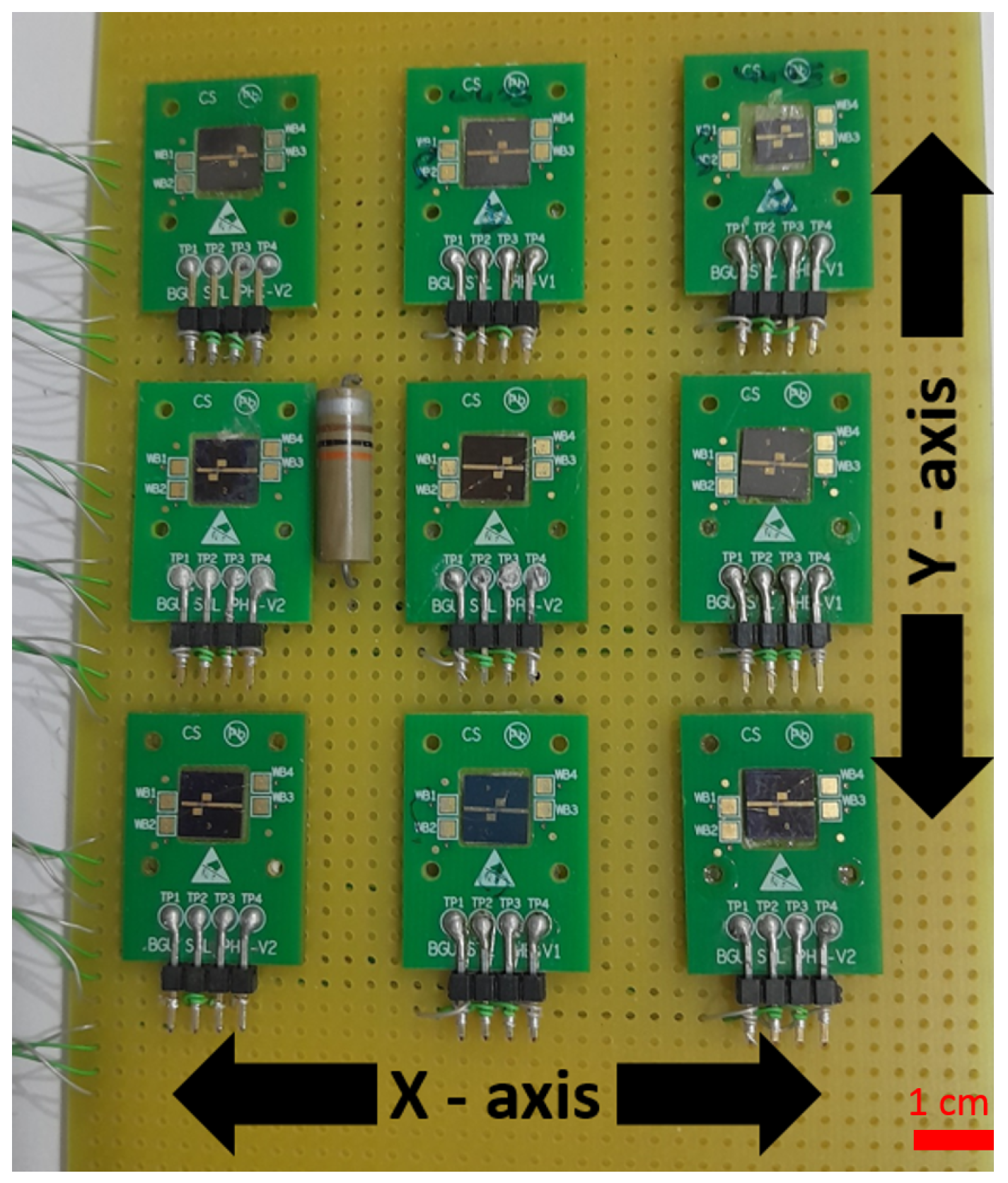
• Use of PHE Sensors for Magnetic Field Mapping: This study is the first to employ PHE sensors in a compact 3 × 3 grid for precise magnetic field mapping, highlighting their potential for high-resolution applications;
• Application of Small Sensors: The use of small elliptical PHE sensors demonstrates their feasibility for constructing dense sensor arrays in constrained environments, such as medical and industrial applications.

The structure of this paper is as follows:

Section 2 details the experimental setup, including the design of the PHE sensor array, the magnetic source, and the data acquisition system. This section also describes the deterministic and machine learning-based data processing methods used. Section 3 provides an in-depth analysis of the experimental and simulation results. This includes the performance of the LMA and the FCNN in reconstructing magnetic field maps, along with a comparison of their effectiveness. Section 4 concludes and explores the implications of the results, emphasizing the scalability and applicability of the proposed methods.

2. Materials and Methods

Our experimental setup consists of a magnetic source, a sensor array that picks up the magnetic signals, and an interface that drives and probes the sensors and processes the signal. In the following, we describe each part of the system.

2.1. The Magnetic Source

The magnetic dipole source is approximated using a miniature coil with a diameter and length of 2.5 mm and 19 mm, respectively. The coil consists of 2783 turns, carrying a sinusoidal current of 50 mA at a fixed frequency of 10 Hz.

2.2. The Magnetic Sensors

The magnetic sensors used in this study are elliptical PHE sensors.

The shape of each sensor induces a uniaxial anisotropy along its easy axis, known as shape anisotropy [29]. The sensitivity of the sensor, $S_y$, is given by

$$S_y=I_x{\displaystyle \frac{\Delta \rho }{t}}{\displaystyle \frac{1}{H_{eff}}}$$

(1)

where $▵\rho$ represents the sensor resistivity anisotropy, $H_{eff}$ is the effective anisotropy field [29,30], t is the sensors’s thickness, and $I_x$ is the applied current (the excitation current that flows along the sensor’s easy axis).

The fabrication process of the sensor involves several steps. Initially, an ion beam sputtering system is used to deposit ${\mathrm{Al}}_2{\mathrm{O}}_3$ (35 nm)/Ta (5 nm)/Py (50 nm)/Ta (5 nm) onto a silicon wafer [31]. During the deposition, a field of 100 Oe is applied to induce uniaxial anisotropy in the sensor [32]. Following this, photolithography is employed to create the elliptical shape of the sensor, along with multiple steps of dry and wet etching. Finally, gold contacts are patterned and created using another round of photolithography, deposition, and dry-etching processes [29].

The typical equivalent magnetic noise (EMN) of the 50 nm thick PHE sensors is ∼ 36 ${\displaystyle \frac{pT}{\sqrt{Hz}}}$ at 10 Hz [30].

The array, as shown in Figure 1, enables the construction of a “magnetic image”, a 2D magnetic heat map that represents the magnetic field in the array’s plane. In this paper we enhance the resolution of these magnetic heat maps using ML algorithms.

2.3. The Interface

In this chapter, we present the experimental setup and techniques underlying our magnetic imaging framework. The system combines a compact 3 × 3 array of PHE sensors with machine learning to overcome spatial resolution constraints. Key components include sensor fabrication, interface, and data processing strategies. Detailed simulations and theoretical calculations guide the application and evaluation of the methodology.

The interface for a single PHE sensor is schematically described in Figure 2. The constant current source (‘VCCS’) module drives current in the longitudinal axis (X-axis) of the sensor. In the transverse axis (Y-axis), the PHE sensor is connected through the amplification module (‘Amp.’) to the demodulation (‘Demodulator’) module. The demodulator is connected to the ADC, while the ADC is connected via $I^{2}C$ communication to the microcontroller. All nine sensors are connected to the control center by SPI communication. The control center (as described in Figure 3) synchronizes the sampling of the nine sensors using a synchronization signal. The control center is connected via USB to the system’s computer for transmitting the readouts of the array.

2.4. Data Processing

In this section, we present two different approaches to process the measured data and create an high resolution heat map from it. The first approach is a deterministic algorithm, the LMA, and the second approach is an ML-based algorithm, FCNN. The initial step for both approaches is preprocessing the data. During the preprocessing stage, the initial phase involves data filtration. The data received by the system contain high-frequency noise, as well as a direct current offset originating from the ADC. To address the DC offset, we employ a detrend technique. As for high frequencies, we used a Butterworth low-pass Infinite Impulse Response (IIR) filter with a basic cut-off of 50 Hz. In addition, it is necessary to implement another filter to eliminate any traces of the carrier wave. This is performed using a smoothing procedure, namely, the Savitzky–Golay filter [33]. For the ML approach, there is a second step in the preprocessing. The second step involves generating a two-dimensional magnetic heat map. We define three distinct categories of magnetic heat maps: theoretical magnetic heat maps, magnetic heat maps derived using simulations of measured magnetic field, and magnetic heat maps obtained using the actual experimental setup.

The purpose of the theoretical and simulated heat maps is to generate data that can be used to train a learning model. This model will predict the intensity and location of the magnetic source in the experimental heat maps.

Theoretical magnetic heat maps are generated using a dense two-dimensional grid measuring 50 mm × 50 mm. The field calculations are performed with a spatial resolution of 1 ${\mathrm{mm}}^2$ and rely on the Biot–Savart law (BSL).

The simulated magnetic maps are generated by positioning a network of simulated sensors over a 50 mm × 50 mm plane—identical to the theoretical maps, but with a much coarser grid—then computing the magnetic field using BSL only at the simulated sensors locations. The heat map is then computed by a two-dimensional interpolation on the same grid used in the theoretical maps calculations. We have tried various methods of two-dimensional interpolation, including cubic spline and Kriging, all of them leading to very similar results. As previously stated, the inclusion of more simulated sensors in the network will enhance the precision of the simulated magnetic heat map. Obviously, the more simulated sensors in the array, the higher the accuracy of the magnetic heat map. After the preprocessing stage is over, we turn to describe each approach separately:

• LMA approach:

• The general problem, solved by LMA [34], can be formulated as

  $$\underset{\mathbf{x}}{min}\sum _{i=1}^m{\left(f_i\left(\mathbf{x}\right)\right)}^2$$

  (2)

  where $f_i\left(\mathbf{x}\right)$ are the residuals, $\mathbf{x}$ is the vector of parameters to be optimized, and m is the size of the data. At each iteration, the LMA updates the current parameter estimate ${\mathbf{x}}_k$ in $\mathbf{x}$. The update rule essentially minimizes a regularized least squares objective, where a damping parameter controls the trade-off between the Gauss–Newton and Gradient Descent methods.
• The LMA is a local scheme that solves the inverse problem of the magnetic field generated by a given source using the data recorded at the sensors. For a current loop, the magnetic moment $\mathbf{m}$ is related to the current I and the area A of the loop. Specifically, the magnetic moment is given by $\mathbf{m}=I\mathbf{A}$. For a circular loop with radius $r_{\mathrm{loop}}$, the area A is $A=\pi r_{\mathrm{loop}}^2$, and the magnetic moment becomes $m=I\pi r_{\mathrm{loop}}^2$. The magnetic field at a point located at a distance r from the current loop (in the far-field or dipole approximation) is

  $$B={\displaystyle \frac{{\mu }_0}{4\pi }}{\displaystyle \frac{m}{r^3}}$$

  (3)

  Substituting the expression for m, we obtain

  $$B={\displaystyle \frac{{\mu }_0}{4\pi }}{\displaystyle \frac{I\pi r_{\mathrm{loop}}^2}{r^3}}$$

  (4)

  where
  • B is the magnetic field at the sensor in Tesla;
  • I is the current in the loop (in amperes);
  • $r_{\mathrm{loop}}$ is the radius of the current loop;
  • $r=\sqrt{x_s^2+y_s^2}$ is the distance from the loop to the sensor located at $(x_s,y_s)$;
  • ${\mu }_0$ is the permeability of free space (${\mu }_0=4\pi \times {10}^{-7}\mathrm{T}·\mathrm{m}/\mathrm{A}$).
• Thus, the magnetic field at the sensor is

  $$B={\displaystyle \frac{{\mu }_{0}I{r}_{\mathrm{loop}}^2}{4r^3}}$$

  (5)

  where $r=\sqrt{{(x-x_s)}^2+{(y-y_s)}^2}$ is the distance from the current loop to the sensor. In our case, we solve a system of nine equations (nine sensors) with three unknowns: the position of the source (x,y) and the current I. This is an overdetermined system of equations that is ready for LMA treatment. Its solution is not a map but a single point. In order to obtain a two-dimensional solution, we develop a three-step strategy:

  (a)

  We divide the cylindrical source into 15 equal sub-sources (see Figure 4);

  (b)

  We solve by LMA for each segment separately and obtain 15 positions and current values;

  (c)

  We build a magnetic heat map by interpolating the field computed at the LMA solution and the recorded field of the 9 senors, using Equation (4) to convert from current to magnetic intensity.

2.

FCNN model training:

• We use a machine learning (ML) methodology for several compelling factors. First, the simulation process allows us to generate a substantial amount of labeled data required by the learning algorithm. Second, the ML approach is inherently powerful due to its ability to train the model without relying on assumptions about the physical model of the problem. This property enables almost any modifications of the problem type and the retraining of the model without compromising its accuracy. Finally, once the model has been trained offline, the real-time predictions are significantly faster compared to any heuristic approaches.
• We chose the FCNN due to its straightforwardness and practicality. The localization problem, i.e., determining the 2D coordinates of the anomaly, may be addressed as a straightforward regression problem. This can be effectively solved using an FCNN, yielding a high level of accuracy.

3. Results

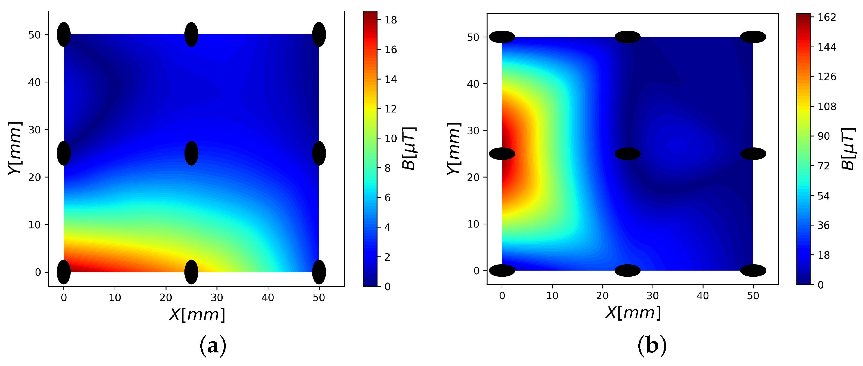
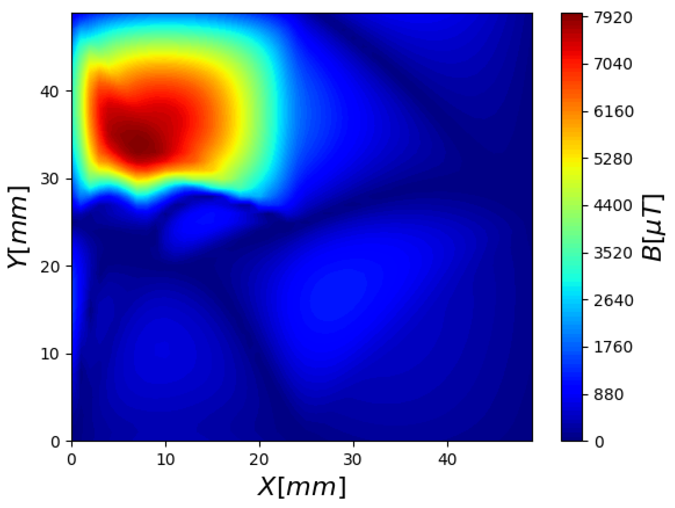
3.1. Theoretical Magnetic Map

We begin by calculating the magnetic map based on the expected values for the magnetic source described in Section 2.1.

Figure 5 shows the calculated magnetic field over a square grid of 5 cm side length, with a spatial resolution of 1 ${\mathrm{mm}}^2$. The position of the center of the coil was set to be (8 $\mathrm{mm}$, 29.5 $\mathrm{mm}$), as shown in Figure 5.

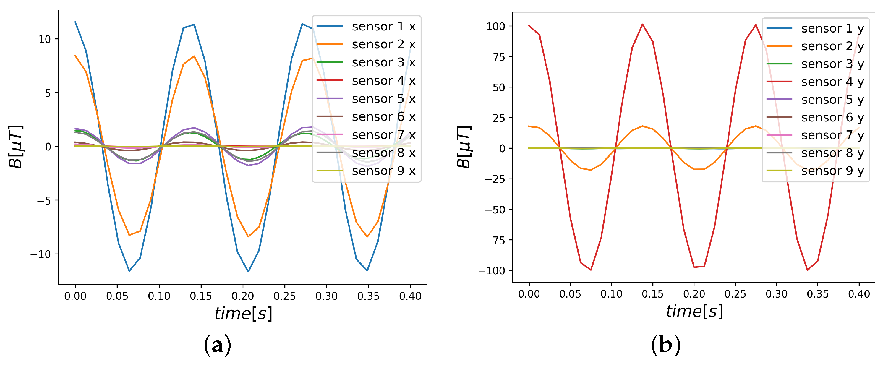
3.2. Measurement Setup of Nine PHE Sensor Array

We now turn to the experimental measurement. The experimental measurement setup is shown in Figure 1. The measurement was carried out in two parts: x-axis measurements and y-axis measurements. In each measurements, we measured the magnetic field in each sensor as a function of time, as shown in Figure 6.

For each sensor in Figure 6, we calculated the root mean square (rms) value of the magnetic field, $B_{IP}=\sqrt{B_{x_{rms}}^2+B_{y_{rms}}^2}$, and from these values we have built a continuous map, using a two-dimensional interpolation on the same dense grid used for the theoretical maps (see Figure 7).

In Figure 8, we show the interpolation of $B_{IP}$ based on the measurements and using the theoretical values of $B_{IP}$ at the same locations.

The maps in Figure 8 are quite similar, as expected, and they both fail to provide a satisfactory representation of the magnetic field map shown in Figure 5.

3.3. Simulations

To study the expected effect of increasing the number of sensors in the same area on the quality of the magnetic field map, we performed simulations using arrays consisting of 50, 500, 1000, and 10,000 sensors, placed on an equidistant two-dimensional mesh. Figure 9 illustrates the results of the these simulations after a 2D interpolation has been performed.

We note that the field map obtained with an array consisting of 50 sensors, as shown in Figure 9a, has its maximum value at coordinates (9, 33), while we expect the maximum to be at the center of the coil, which is (8, 29.5). In addition, the overall map is still quite different from Figure 5. Only after further increasing the array to 1000 sensors, the shape of the coil starts emerging (Figure 9c). By increasing the number of sensors by another factor of magnitude, one is able to reconstruct the full magnetic map (Figure 9d).

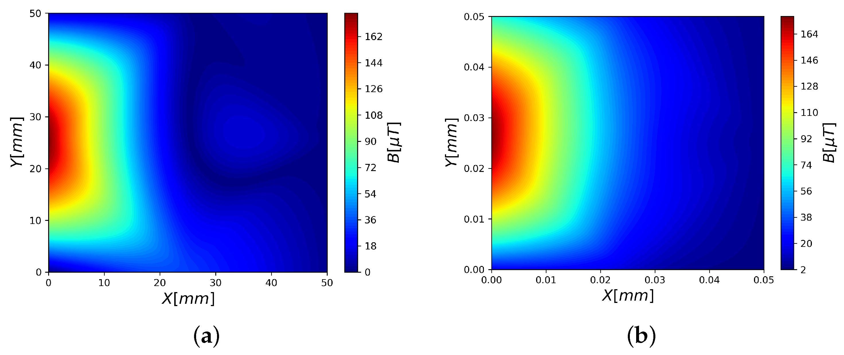
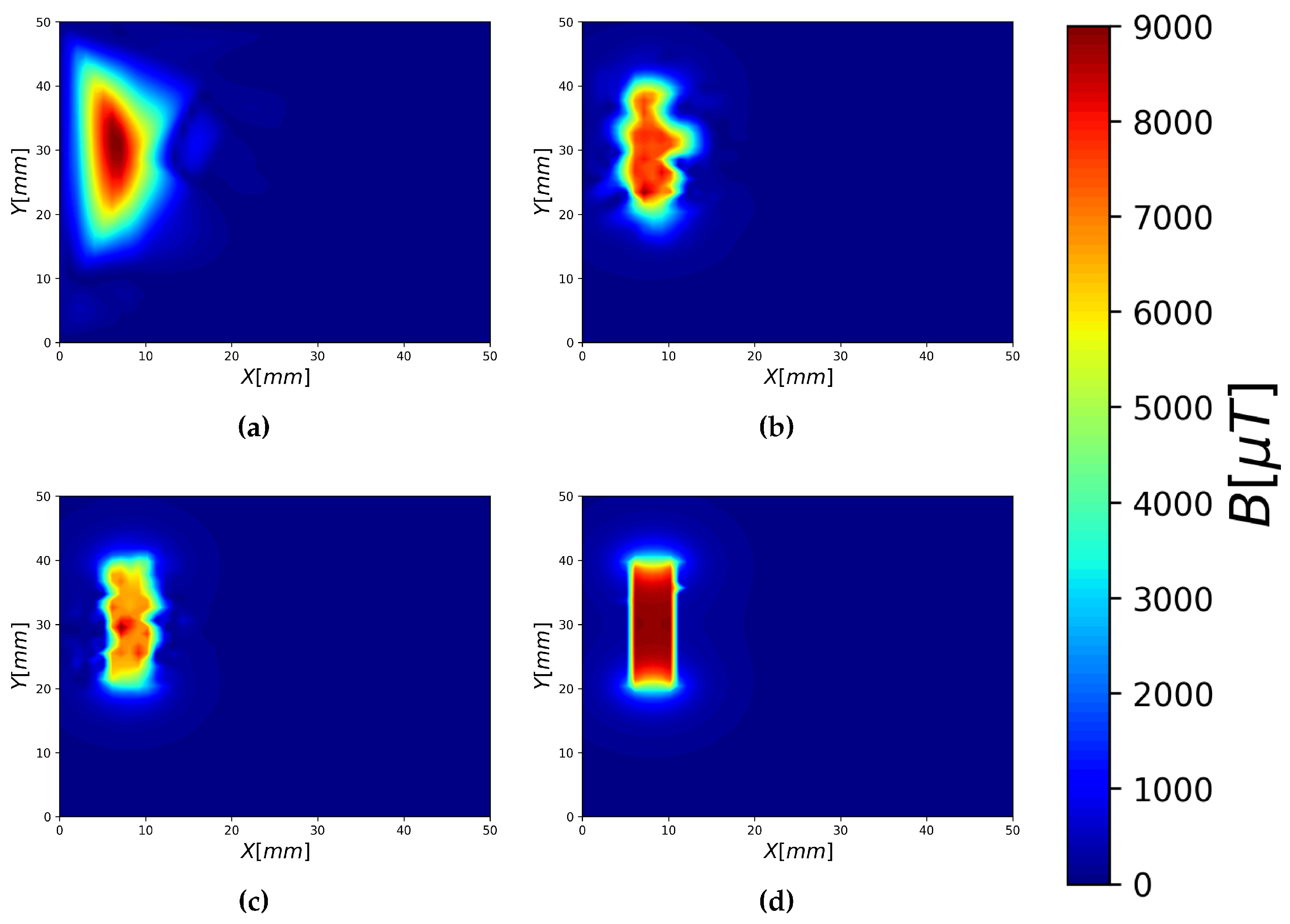
3.4. Mapping Using LMA Approach

The LMA was utilized to determine the magnetic source’s location and parameters by minimizing the discrepancy between the theoretical and experimental magnetic field data. The algorithm iteratively adjusted the source’s position and current until the residuals converged to a satisfactory level. Using nine PHE sensors in a 3 × 3 grid, the LMA estimated the centers of each segment of the coil with reasonable accuracy, as illustrated in Figure 10b. The real center of each segment of the coil is illustrated in Figure 10a.

Based on the magnetic values produced by the LMA and the nine measurement points, we calculated the magnetic heat map. This heat map, as shown in Figure 11, shows some improvement over the heat map that is based on the measurement (Figure 8a).

However, the sparsity of the sensor data led to significant deviations in the reconstructed field map, emphasizing the limitations of traditional optimization methods for sparse sensor arrays. The initial guess for the algorithm, set to (25, 25, 1), was chosen as the center of the 50 mm × 50 mm plane, assuming that the source is approximately at the center due to its symmetric placement and for simplicity in calculations. Each coordinate took 15 ms to calculate with this algorithm. In general, for 15 points, the total run time of this algorithm is 45 ms. This approach aimed to reduce the likelihood of convergence issues by starting at a neutral point with respect to the array geometry. For setups with multiple magnetic sources, the algorithm’s performance significantly degrades due to its reliance on single-source assumptions, making it challenging to resolve overlapping fields or distinguish between closely located sources. Compared to the ML method, LMA is constrained by its need for a good initial guess and struggles with complex, non-linear relationships in data. Moreover, the ML approach excels in handling multiple sources and extracting richer spatial information, offering superior flexibility and spatial resolution.

The reconstruction of the magnetic field map using the LMA involved two key approaches illustrated in Figure 11. Here, the magnetic field map is derived based on the estimated source parameters obtained from the algorithm, ignoring direct sensor measurements. This approach highlights the limitations of LMA when interpolating sparse sensor data, as the reconstructed map often deviates from the expected spatial profile due to the algorithm’s reliance on the estimated parameters alone. In contrast, the image in Figure 11 represents a 2D interpolation that combines the results of the LMA with the measured magnetic field values from the nine PHE sensors. By integrating these measurements, the map retains features influenced directly by the experimental data, offering a more accurate representation of the field. However, while this combined approach improves fidelity, the sparse sensor grid still limits the resolution, and the map remains unable to capture finer spatial details of the magnetic field. This reinforces the need for additional sensors or advanced methods, such as ML-based techniques, to enhance the spatial accuracy of the reconstruction.

3.5. Mapping Using ML Approach

Here, we show that data obtained from nine sensors can yield a much better magnetic field mapping when ML algorithms are used. We use a dedicated FCNN, which learns the map created by a cylinder-shaped coil from many different simulations of nine-sensor array data. For each simulation, we also calculate the theoretical magnetic heat map, so the FCNN uses the theoretical magnetic heat map as labels for the simulation.

3.5.1. FCNN Model Training

The training and validation set consist of encoded magnetic heat maps, where the precise position of the coil’s center is indicated by the matching theoretical magnetic heat maps. For training purposes, we utilized a diverse range of encoded images with varying numbers of sensors, along with different coil positions and various magnetic moments. This is carried out to prevent overfitting. We mostly utilize experimental heat maps in the test set, along with synthetic heat maps.

• FCNN meta parameters:
  We implement our network in Python using PyTorch. The network architecture consists of an input layer with 2500 neurons, 2 hidden layers (the first has 750 neurons and the second has 500 neurons), and an output layer, which has 2500 neurons. The total number of trainable parameters in the network is 3,503,750. The Adam optimization method with a learning rate of $\alpha =0.01$ was chosen. The training process involves a total of 2000 simulations.
  These simulations were restricted in a two-dimensional area of 50 mm × 50 mm. In each simulation, the following parameters were randomly chosen according to a normal distribution:
  • The coordinates of the center of mass of the coil, $(X_{cm},Y_{cm})$;
  • The orientation of the coil in the x–y plane, $\theta$;
  • The length of the coil, l;
  • The current intensity, I.
  The mean and the variance for each parameter are given in

  Table 1. Mean and standard deviation of the parameters based on their uniform distributions.

  Parameter	Mean	Standard Deviation
  ${\overrightarrow{R}}_{cm}$ (mm)	$35.355$	$10.202$
  $\theta$ (radians)	$\pi$	$1.813$
  l (mm)	$20.0$	$2.886$
  I (mA)	$50.5$	$28.589$

  .
  The training process was conducted for a total of 200 epochs using NVIDIA A100, with cuda version 12.1.
  The process is shown in Figure 12. It took 25 min of CPU time, and testing the network with our measurements (the measurements are equal to 1 simulation in size) took 20 ms. The final step is to test the model with experimental data (the magnetic heat map on the left side of Figure 8).
• Loss function:
  For training the FCNN we decided to use a loss function that combines a global and a local estimation error. The purpose was optimizing the network convergence from the full heat map point of view but still emphasizing the most significant physical structure, namely, the coil’s center of mass, which can be considered as an anchor point.
  The global part of the loss function is given by the Structural Similarity Index Measure (SSIM) [35]. Unlike traditional metrics such as mean squared error (MSE) or peak signal-to-noise ratio (PSNR), which primarily focus on pixel-wise differences, SSIM considers changes in structural information, luminance, and contrast. This often makes it more aligned with human visual perception. SSIM is a combination of luminance, contrast, and structure. We chose the SSIM components’ adjustment parameters to be $\alpha =\beta =\gamma =1$.
  The local term of the loss function, noted as $L{F}_{net}$, is defined by

  $$L{F}_{net}={({\overrightarrow{\rho }}_{pred}-{\overrightarrow{\rho }}_{theoretical})}^2$$

  (6)

  where ${\overrightarrow{\rho }}_{pred}$ is the center of mass of the coil predicted by the FCNN, and ${\overrightarrow{\rho }}_{theoretical}$ is its theoretical, i.e., exact, position. We summarize this hybrid loss function in the following expression:

  $$\begin{array}{c}\hfill Loss={\lambda }_1(1-SSIM)+{\lambda }_{2}L{F}_{net}\end{array}$$

  (7)

  where $0\le {\lambda }_1$, ${\lambda }_2\le 1$, and ${\lambda }_1+{\lambda }_2=1$.

3.5.2. Prediction Results

From now on, the prediction presented here is solely based on the measurement, as shown in Figure 8a as a test case, and we stop using simulations. We trained the network using only a global and no local contribution (${\lambda }_1=1$, ${\lambda }_2=0$). We tested the trained FCNN model with our measurement as input, in order to obtain the true shape and position of the coil in our measurement or, in other words, “detect” the coil in the measurement. The goal was to achieve a prediction that would resemble, as much as possible, the theoretical magnetic heat map (Figure 5). The trained model prediction is shown in Figure 13.

We trained the network four additional times with varying global and local contributions: ${\lambda }_1=0.5$, ${\lambda }_2=0.5$; ${\lambda }_1=0.25$, ${\lambda }_2=0.75$; ${\lambda }_1=0.1$, ${\lambda }_2=0.9$; and ${\lambda }_1=0$, ${\lambda }_2=1$. Each trained FCNN model was tested using our measurement as input, consistent with the previously stated rationale. The trained model’s predictions are shown in Figure 14.

All the predicted heat maps resemble the theoretical heat map (Figure 5). The magnetic heat map predicted by the FCNN trained with the loss function parameters ${\lambda }_1=1,{\lambda }_2=0$ (Figure 13) most closely reproduced the shape of the magnetic object. However, the other magnetic heat maps (Figure 14a–d) achieved significantly smaller offsets in the coil’s center coordinates, as shown in

Table 2. MSE calculations and coordinate offsets for different loss functions. The worst values are colored red, and the best values are colored blue.

Loss Function		Results
${\mathbf{\lambda }}_{\mathbf{1}}$	${\mathbf{\lambda }}_{\mathbf{2}}$	MSE Value	X Offset (mm)	Y Offset (mm)
1.0	0.0	2.4615	0.5	1.02
0.5	0.5	2.6621	0.162	0.9
0.25	0.75	2.6484	0.157	0.051
0.1	0.9	2.5768	0.145	0.045
0.0	1.0	2.467	0.142	0.042

(with the highest offset marked in red and the lowest in blue). Finally, we also calculated the MSE between the theoretical heat map and the predicted heat maps in order to quantitatively estimate the matching of the predicted heat maps to the theoretical heat map, as shown in Table 2.

Intuitively, the prediction that is based on a trained model with loss function that has ${\lambda }_1=1$, ${\lambda }_2=0$ should visually be the most similar to the theoretical heat map. As it turns out, the prediction of the trained model with the loss function that has ${\lambda }_1=1$, ${\lambda }_2=0$ (Figure 13) is the most similar to the theoretical heat map, by the MSE metric that we used (marked as blue in Table 2), and the prediction of the trained model with the loss function that has ${\lambda }_{0.5}=1$, ${\lambda }_2=0.5$ (Figure 14a) is the least similar (marked as red in Table 2) to the theoretical heat map. We were successful in achieving the proper arrangement of the coil, and the overall topography relative values have also been accurately restored. The final result is quite promising, as the form and general topography now closely resemble the one achieved through a simulation with 1000 sensors (see Figure 9c).

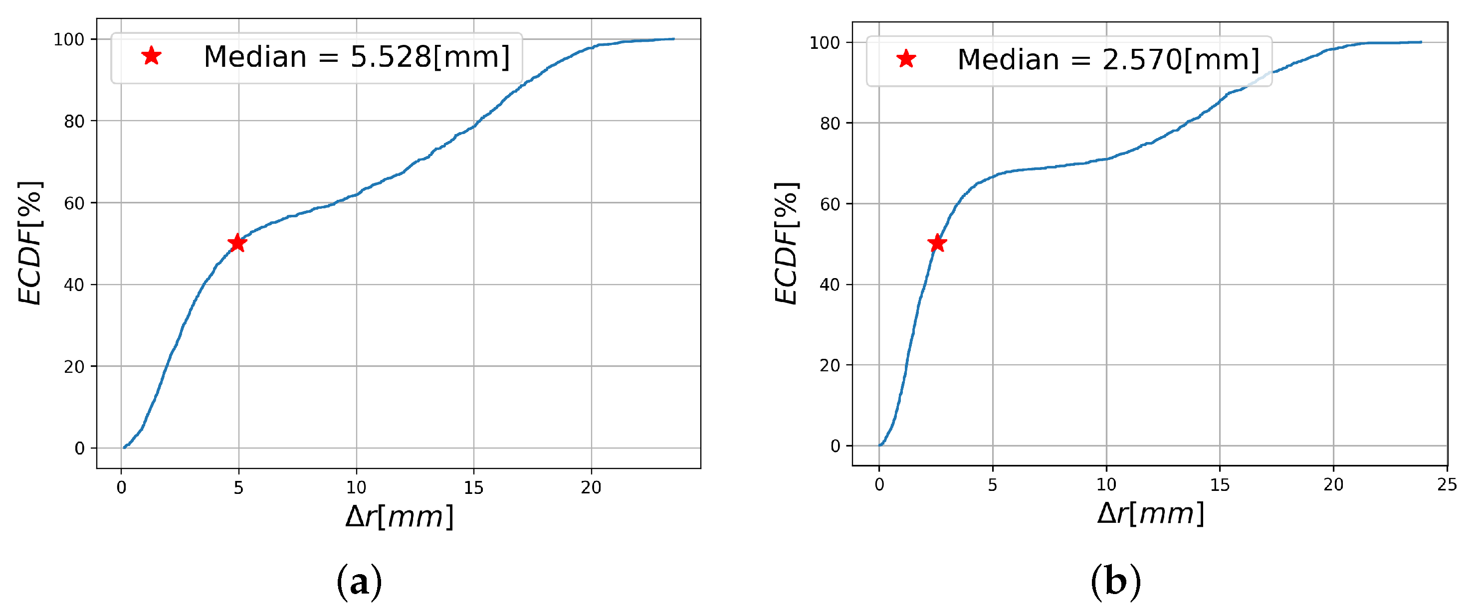
3.5.3. Performance of the ML Model Against Simulated Measurements

Until now, we have developed a deep learning network and tested it against one single real-life experimental configuration. Conducting hundreds, if not thousands, of such tests to measure the model’s performance is not actually realistic. However, a first estimation of the model performance can be obtained if one replaces the real-life experiment by suitable simulations. For this purpose, we created a new database of 4800 simulations, in which we kept the coil’s length and the current intensity constant, to stay as close as possible to the real-life measurement setup. The other two variables, namely, the coil’s position and its orientation, were varied in order to cover the full test space without passing through the boundaries of the perimeter.

The model was then applied to each of the simulations, providing a prediction that was compared to the true, exact position and orientation of the coil.

Let us define $\Delta r$ by

$$\begin{array}{c}\hfill \Delta r=|\Delta \overrightarrow{r}|=|{\overrightarrow{r}}_{prediction}-{\overrightarrow{r}}_{simulation}|\end{array}$$

(8)

and $\Delta \theta$ as

$$\begin{array}{c}\hfill \Delta \theta =|{\theta }_{prediction}-{\theta }_{simulation}|\end{array}$$

(9)

where ${\overrightarrow{r}}_{simulation}$ is equivalent to ${\overrightarrow{r}}_{measurement}$ in the previous section, ${\theta }_{simulation}$ is the calculated orientation in the tests images, and ${\overrightarrow{r}}_{prediction}$ and ${\theta }_{prediction}$ are the vector position and the orientation predicted by the FCNN model. The performance of the model with respect to $\Delta r$ and $\Delta \theta$ can be estimated using the Empirical Cumulative Distribution Function (ECDF). This function estimates the probability that, in a reconstructed magnetic field containing a strong source like a coil, the center of mass of this coil will not deviate from its true position by more than $\Delta r$ and from its true orientation by $\Delta \theta$. The model tested was trained with the loss functions ${\lambda }_1=1$, ${\lambda }_2=0$ and ${\lambda }_1=0$, ${\lambda }_2=1$.

In Figure 15a, we mark the median of $\Delta r$ using a red star at 5.528 mm. Taking into account the length of the coil and the fact that the coil cannot cross the perimeter boundaries, this value can be converted into a localization error of approximately 15.6%. In Figure 15b, the median of $\Delta r$ is 2.57 mm, resulting in a localization error of approximately 7.2%.

As far as the orientation is concerned, we plot the ECDF for $\Delta \theta$ in Figure 16. Here too, we consider two extreme cases of loss functions with respect to the relative weights of the global and local terms.

An important remark should be made here. The second parameter that we used to generate the various scenarios of the database is the angle $\theta$ made by the rectangular coil with the x-axis. Although the original angle is a well-known value (input), the “predicted” angle is not trivially calculated. From the magnetic field picture we need to extract the angle between the long axis of the pattern and the x-axis. This was achieved by running a Radon transform [36] that searches and analyzes ellipse-shaped patterns. The Radon transform is a mathematical operation that transforms a 2D image into a set of projections used for tasks like image reconstruction and pattern recognition. When applied to elliptical shapes, the Radon transform helps to identify the parameters (e.g., the center, axes, and orientation) of the ellipse in the image. The Radon transform $R\left\{f\right\}(\rho ,\theta )$ of a function $f(x,y)$ is given by the following integral:

$$R\left\{f\right\}(\rho ,\theta )={\int }_{-\infty }^{\infty }f(x,y)\delta (xcos\theta +ysin\theta -\rho )dxdy$$

where

• $f(x,y)$ is the original image function;
• $\rho$ is the perpendicular distance from the origin to the line of projection;
• $\theta$ is the angle of projection relative to the x-axis;
• $\delta (xcos\theta +ysin\theta -\rho )$ is the Dirac delta function that constrains the projection to a particular line at a distance $\rho$.

The Radon transform accumulates the projection of the intensity values along the lines at different angles $\theta$. It then produces a heat map in which the local maximum corresponds to the main parameters of the ellipse, in particular, the angle $\theta$ that we are looking for.

In Figure 16a, we use the median of $\Delta \theta$ to calculate the orientation error, taking into account the maximum possible rotation, which is 360°, we obtain an error of approximately 13%. In Figure 16b, the error is approximately 2.5%.

We believe that these errors, both localization and orientation, can be further reduced by using more sophisticated models, such as the ‘pix2pix’ method [37], or advanced ML techniques such as the Super Resolution Generative Adversarial Network (SRGAN) [38].

4. Conclusions

This study addresses the challenge of precise magnetic field mapping with minimal hardware, leveraging a sparse array of PHE sensors. By integrating traditional optimization techniques with machine learning, the research provides an innovative approach to enhance spatial resolution without increasing the sensor density.

We introduce a novel method for quantifying the magnetic field using PHE sensors, as well as conducting measurements with numerous sensors (an array of sensors) to generate a magnetic heat map. In order to further improve the resolution of our magnetic map, we developed dedicated machine learning models that use simulated measurements from an array of sensors to learn the theoretical magnetic heat map of the specific unit under test and the distortion of the field that it generates.

The findings reported in this research demonstrate that employing ML yields equivalent resolution for a measured magnetic heat map compared to the one obtained using a significantly larger number of sensors. The FCNN outperforms deterministic methods in accuracy and flexibility, achieving resolutions comparable to a much denser sensor arrays. The findings suggest that advanced ML models can effectively reconstruct magnetic fields, making them a promising tool for applications requiring minimal hardware.

However, while the results show clear improvements in spatial resolution and efficiency, there are inherent trade-offs associated with this approach. The reliance on simulated data for neural network training introduces a dependency on the accuracy and representativeness of the simulations. Any deviations between the simulated and experimental conditions may lead to inaccuracies in the heat map generation. Additionally, the sparsity of the sensor array, while innovative, inherently limits the granularity of the raw data, requiring robust interpolation methods to reconstruct the magnetic field. This places significant demand on the ML model’s ability to generalize and accurately infer details that are not explicitly captured by sensor measurements.

Future work could focus on validating the robustness of the ML approach using diverse experimental conditions and investigating hybrid strategies that combine ML with additional sparse measurements to balance accuracy and resource efficiency. In future work, our objective is to enhance the quantitative accuracy of the magnetic heat map while also achieving a precise estimation of the magnetic object’s location. This could have several applications, such as identifying and differentiating multiple magnetic objects on a map, as well as determining the geometric characteristics of the anomalies. A possible solution could, for instance, integrate the ‘pix2pix’ method, as described in the study by Henry et al. [37]. A significant challenge lies in effectively training the model due to the requirement of a large and diverse dataset. Other future work includes optimizing the ratio of space size to sensor count to balance accuracy and cost-efficiency; adapting the method for varied magnetic object geometries, dimensions, and materials to ensure versatility; and exploring advanced ML techniques such as the Super Resolution Generative Adversarial Network (SRGAN) [38] to further refine field reconstructions.

References

1. Zuo, S.; Heidari, H.; Farina, D.; Nazarpour, K. Miniaturized magnetic sensors for implantable magnetomyography. Adv. Mater. Technol. 2020, 5, 2000185. [Google Scholar] [CrossRef]
2. Saha, R.; Tonini, D.; Hopper, M.S.; Goyal, A.; Yuen, J.; Oh, Y.; Sanger, Z.; Faramarzi, S.; Shiao, M.; Van Helden, D.; et al. Micromagnetic Neural Stimulation and Spintronic Neural Sensing. In Proceedings of the 2024 IEEE International Magnetic Conference-Short Papers (INTERMAG Short Papers), Rio de Janeiro, Brazil, 5–10 May 2024; IEEE: Piscataway, NJ, USA, 2024; pp. 1–2. [Google Scholar]
3. Fu, Q.; Wang, X.; Guo, J.; Guo, S.; Cai, Z. Magnetic Localization Technology of Capsule Robot Based on Magnetic Sensor Array. In Proceedings of the 2020 IEEE International Conference on Mechatronics and Automation (ICMA), Beijing, China, 13–16 October 2020; Volume 10, pp. 267–272. [Google Scholar] [CrossRef]
4. Huang, G.W.; Jeng, J.T. Implementation of 16-channel AMR sensor array for quantitative mapping of two-dimension current distribution. IEEE Trans. Magn. 2018, 54, 1–5. [Google Scholar] [CrossRef]
5. Ye, C.; Wang, Y.; Wang, M.; Udpa, L.; Udpa, S.S. Frequency domain analysis of magnetic field images obtained using TMR array sensors for subsurface defect detection and quantification. NDT E Int. 2020, 116, 102284. [Google Scholar] [CrossRef]
6. Wu, Z.; Huang, H.; Zhao, G.; Liu, J. TMR-Array-Based Pipeline Location Method and Its Realization. Sustainability 2023, 15, 9816. [Google Scholar] [CrossRef]
7. Chen, C.H.; Chen, P.W.; Chen, P.J.; Liu, T.H. Indoor positioning using magnetic fingerprint map captured by magnetic sensor array. Sensors 2021, 21, 5707. [Google Scholar] [CrossRef]
8. Munschy, M.; Boulanger, D.; Ulrich, P.; Bouiflane, M. Magnetic mapping for the detection and characterization of UXO: Use of multi-sensor fluxgate 3-axis magnetometers and methods of interpretation. J. Appl. Geophys. 2007, 61, 168–183. [Google Scholar] [CrossRef]
9. Christou, C.T.; Jacyna, G.M. Vehicle detection and localization using Unattended Ground Magnetometer Sensors. In Proceedings of the 2010 13th International Conference on Information Fusion, Edinburgh, UK, 26–29 July 2010; pp. 1–8. [Google Scholar] [CrossRef]
10. Yoshiaki, A.; Shigenori, K.; Jun, H.; Yoshinori, O.; Yoshihisa, N.; Taishi, W.; Yuki, M.; Gen, U. Multichannel SQUID magnetoneurograph system for functional imaging of spinal cords and peripheral nerves. IEEE Trans. Appl. Supercond. 2021, 31, 1600405. [Google Scholar]
11. Kim, J.; Lee, J.; Jun, J.; Le, M.; Cho, C. Integration of Hall and giant magnetoresistive sensor arrays for real-time 2-D visualization of magnetic field vectors. IEEE Trans. Magn. 2012, 48, 3708–3711. [Google Scholar] [CrossRef]
12. Ribeiro, P.; Neto, M.; Cardoso, S. Strategy for determining a magnet position in a 2-D space using 1-D sensors. IEEE Trans. Magn. 2018, 54, 9401605. [Google Scholar] [CrossRef]
13. Miao, L.; Zhang, T.; Zuo, C.; Chen, Z.; Yang, X.; Ouyang, J. A Rapid Localization Method Based on Super Resolution Magnetic Array Information for Unknown Number Magnetic Sources. Sensors 2024, 24, 3226. [Google Scholar] [CrossRef]
14. Xiao, C.; Liu, S.; Zhou, G.h. Real-time localization of a magnetic object with total field data. In Proceedings of the 2008 World Automation Congress, Waikoloa, HI, USA, 28 September–2 October 2008; IEEE: Piscataway, NJ, USA, 2008; pp. 1–4. [Google Scholar]
15. Alimi, R.; Fisher, E.; Nahir, K. In Situ Underwater Localization of Magnetic Sensors Using Natural Computing Algorithms. Sensors 2023, 23, 1797. [Google Scholar] [CrossRef]
16. Yang, W.; Hu, C.; Meng, M.Q.H.; Song, S.; Dai, H. A six-dimensional magnetic localization algorithm for a rectangular magnet objective based on a particle swarm optimizer. IEEE Trans. Magn. 2009, 45, 3092–3099. [Google Scholar]
17. Song, S.; Hu, C.; Meng, M.Q.H. Multiple objects positioning and identification method based on magnetic localization system. IEEE Trans. Magn. 2016, 52, 9600204. [Google Scholar] [CrossRef]
18. Hu, S.; Tang, J.; Ren, Z.; Chen, C.; Zhou, C.; Xiao, X.; Zhao, T. Multiple underwater objects localization with magnetic gradiometry. IEEE Geosci. Remote. Sens. Lett. 2018, 16, 296–300. [Google Scholar] [CrossRef]
19. Pham, D.M.; Aziz, S.M. A real-time localization system for an endoscopic capsule. In Proceedings of the 2014 IEEE Ninth International Conference on Intelligent Sensors, Sensor Networks and Information Processing (ISSNIP), Singapore, 21–24 April 2014; IEEE: Piscataway, NJ, USA, 2014; pp. 1–6. [Google Scholar]
20. Ouyang, G.; Abed-Meraim, K. A Survey of Magnetic-Field-Based Indoor Localization. Electronics 2022, 11, 864. [Google Scholar] [CrossRef]
21. Ouyang, G.; Abed-Meraim, K. Analysis of Magnetic Field Measurements for Indoor Positioning. Sensors 2022, 22, 4014. [Google Scholar] [CrossRef]
22. Fan, L.; Kang, C.; Wang, H.; Hu, H.; Zhang, X.; Liu, X. Adaptive Magnetic Anomaly Detection Method Using Support Vector Machine. IEEE Geosci. Remote. Sens. Lett. 2022, 19, 8001705. [Google Scholar] [CrossRef]
23. Ashraf, I.; Hur, S.; Park, Y. Application of Deep Convolutional Neural Networks and Smartphone Sensors for Indoor Localization. Appl. Sci. 2019, 9, 2337. [Google Scholar] [CrossRef]
24. Galván-Tejada, C.E.; Zanella-Calzada, L.A.; García-Domínguez, A.; Magallanes-Quintanar, R.; Luna-García, H.; Celaya-Padilla, J.M.; Galván-Tejada, J.I.; Vélez-Rodríguez, A.; Gamboa-Rosales, H. Estimation of indoor location through magnetic field data: An approach based on convolutional neural networks. ISPRS Int. J. Geo-Inf. 2020, 9, 226. [Google Scholar] [CrossRef]
25. Liu, T.; Wu, T.; Wang, M.; Fu, M.; Kang, J.; Zhang, H. Recurrent Neural Networks based on LSTM for Predicting Geomagnetic Field. In Proceedings of the 2018 IEEE International Conference on Aerospace Electronics and Remote Sensing Technology (ICARES), Singapore, 4–7 December 2018; pp. 1–5. [Google Scholar] [CrossRef]
26. Jang, H.J.; Shin, J.M.; Choi, L. Geomagnetic Field Based Indoor Localization Using Recurrent Neural Networks. In Proceedings of the GLOBECOM 2017—2017 IEEE Global Communications Conference, Singapore, 4–8 December 2017; pp. 1–6. [Google Scholar] [CrossRef]
27. Chen, S.; Zhu, M.; Zhang, Q.; Cai, X.; Bo, X. Accurate magnetic object localization using artificial neural network. In Proceedings of the 2019 15th International Conference on Mobile Ad-Hoc and Sensor Networks (MSN), Shenzhen, China, 11–13 December 2019; pp. 25–30. [Google Scholar]
28. Zhang, Y.; Lee, J.; Wainwright, M.; Jordan, M.I. On the learnability of fully-connected neural networks. In Proceedings of the 20th International Conference on Artificial Intelligence and Statistics, Fort Lauderdale, FL, USA, 20–22 April 2017; Volume 54, pp. 83–91. [Google Scholar]
29. Lahav, D.; Schultz, M.; Amrusi, S.; Grosz, A.; Klein, L. Planar Hall Effect Magnetic Sensors with Extended Field Range. Sensors 2024, 24, 4384. [Google Scholar] [CrossRef] [PubMed]
30. Nhalil, H.; Das, P.T.; Schultz, M.; Amrusi, S.; Grosz, A.; Klein, L. Thickness dependence of elliptical planar Hall effect magnetometers. Appl. Phys. Lett. 2020, 117, 262403. [Google Scholar] [CrossRef]
31. Gehanno, V.; Freitas, P.P.; Veloso, A.; Ferrira, J.; Almeida, B.; Soasa, J.; Kling, A.; Soares, J.; Da Silva, M. Ion beam deposition of Mn-Ir spin valves. IEEE Trans. Magn. 1999, 35, 4361–4367. [Google Scholar] [CrossRef]
32. Nhalil, H.; Givon, T.; Das, P.T.; Hasidim, N.; Mor, V.; Schultz, M.; Amrusi, S.; Klein, L.; Grosz, A. Planar Hall effect magnetometer with 5 pT resolution. IEEE Sensors Lett. 2019, 3, 2501904. [Google Scholar] [CrossRef]
33. Krishnan, S.R.; Seelamantula, C.S. On the selection of optimum Savitzky-Golay filters. IEEE Trans. Signal Process. 2012, 61, 380–391. [Google Scholar] [CrossRef]
34. Marquardt, D.W. An algorithm for least-squares estimation of nonlinear parameters. J. Soc. Ind. Appl. Math. 1963, 11, 431–441. [Google Scholar] [CrossRef]
35. Wang, Z.; Bovik, A.C.; Sheikh, H.R.; Simoncelli, E.P. Image quality assessment: From error visibility to structural similarity. IEEE Trans. Image Process. 2004, 13, 600–612. [Google Scholar] [CrossRef] [PubMed]
36. Brady, M.L. A fast discrete approximation algorithm for the Radon transform. SIAM J. Comput. 1998, 27, 107–119. [Google Scholar] [CrossRef]
37. Henry, J.; Natalie, T.; Madsen, D. Pix2pix Gan for Image-to-Image Translation; Research Gate Publication: Berlin, Germany, 2021; pp. 1–5. [Google Scholar]
38. Xiong, Y.; Guo, S.; Chen, J.; Deng, X.; Sun, L.; Zheng, X.; Xu, W. Improved SRGAN for remote sensing image super-resolution across locations and sensors. Remote. Sens. 2020, 12, 1263. [Google Scholar] [CrossRef]
Figure 1. The array of PHE sensors.
Applsci 15 00964 g001
Figure 2. The relevant interface for a single PHE sensor.
Applsci 15 00964 g002
Figure 3. System communication network diagram.
Applsci 15 00964 g003
Figure 4. The magnetic source segmented into 15 sub-sources, each one located at ( x i , y j ) , according to its position in the cylinder. The three dots (“...”) in the plot represent values that follow a consistent pattern, they are continuing in the same way as previous ones and are not shown for simplicity or brevity.
Applsci 15 00964 g004
Figure 5. The theoretical magnetic heat map.
Applsci 15 00964 g005
Figure 6. Magnetic field vs. time: (a) B x , (b) B y . Notice that some curves listed in the legend are not visible since their magnitudes are much smaller compared to the other signals. They all fall within the zero line (x axis).
Applsci 15 00964 g006
Figure 7. The magnetic field, calculated based on nine measurements and 2D interpolation, (a) B x , (b) B y . The black ellipses represent the PHE sensors in this measurement.
Applsci 15 00964 g007
Figure 8. A 2D interpolation based on 9 experimental (a) and theoretical (b) values of B I P .
Applsci 15 00964 g008
Figure 9. A 2D interpolation of B I P based on theoretical values assuming an array consisting of 50 (a), 500 (b), 1000 (c), and 10,000 (d) sensors.
Applsci 15 00964 g009
Figure 10. Coil locations: (a) Real, (b) Estimated with the LMA.
Applsci 15 00964 g010
Figure 11. The full reconstructed magnetic heat map using LMA.
Applsci 15 00964 g011
Figure 12. Loss function training and validation curves over 200 epochs. λ 1 = 1 , λ 2 = 0 .
Applsci 15 00964 g012
Figure 13. Visualization of FCNN prediction with loss function parameters λ 1 = 1 , λ 2 = 0 .
Applsci 15 00964 g013
Figure 14. (a) FCNN prediction with loss function parameters λ 1 = 0.5 , λ 2 = 0.5 ; (b) FCNN prediction with loss function parameters λ 1 = 0.25 , λ 2 = 0.75 ; (c) FCNN prediction with loss function parameters λ 1 = 0.1 , λ 2 = 0.9 ; (d) FCNN prediction with loss function parameters λ 1 = 0 , λ 2 = 1 .
Applsci 15 00964 g014
Figure 15. Empirical cumulative distribution function (ECDF) of (a) Δ r for the trained model with loss function that has λ 1 = 1 , λ 2 = 0 , (b) Δ r for the trained model with loss function that has λ 1 = 0 , λ 2 = 1 .
Applsci 15 00964 g015
Figure 16. ECDF of (a) Δ θ for the trained model with loss function that has λ 1 = 1 , λ 2 = 0 , (b) Δ θ for the trained model with loss function that has λ 1 = 0 , λ 2 = 1 .
Applsci 15 00964 g016