

A Bionic Social Learning Strategy Pigeon-Inspired Optimization for Multi-Unmanned Aerial Vehicle Cooperative Path Planning


Abstract
1. Introduction
2. Bionic Social Learning Strategy Pigeon-Inspired Optimization
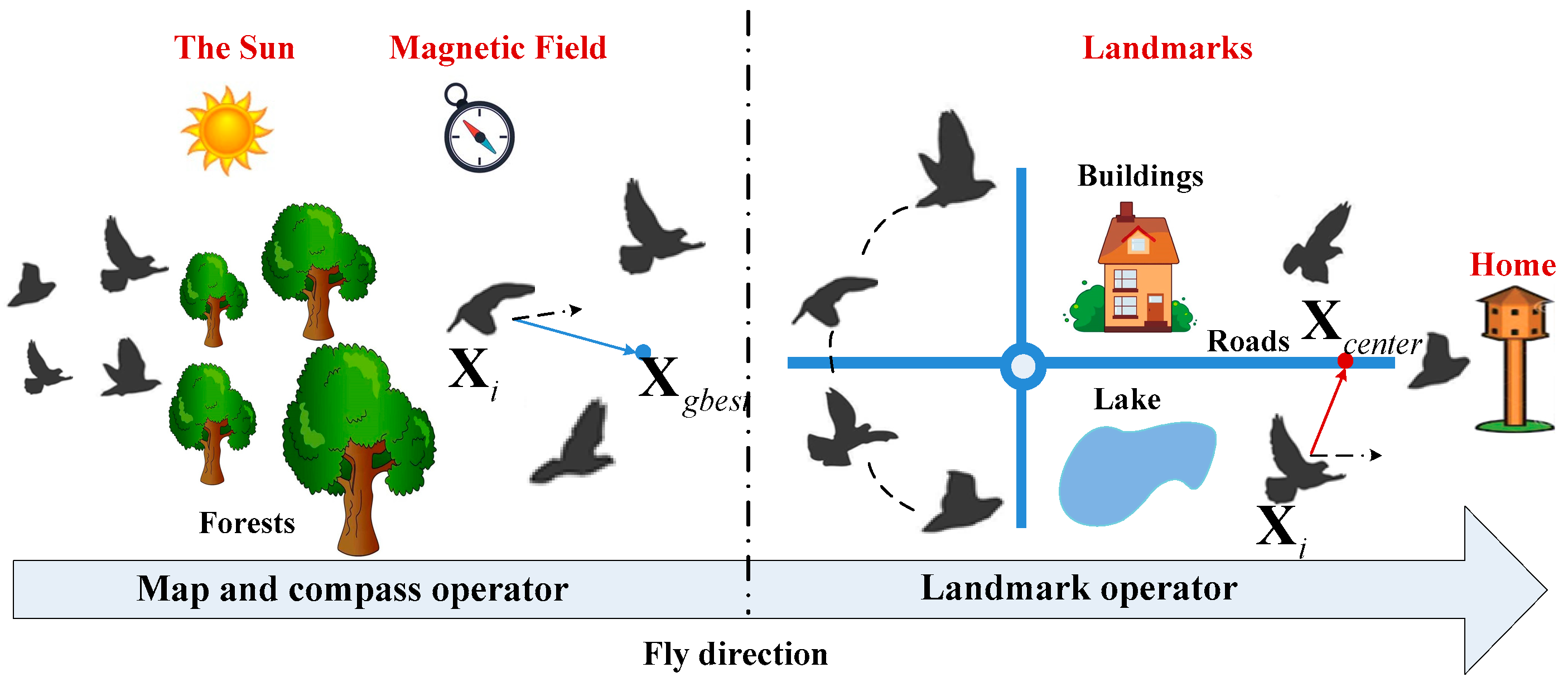
2.1. Review of Standard Pigeon-Inspired Opimization
- Map and compass operator:
- Landmark operator:
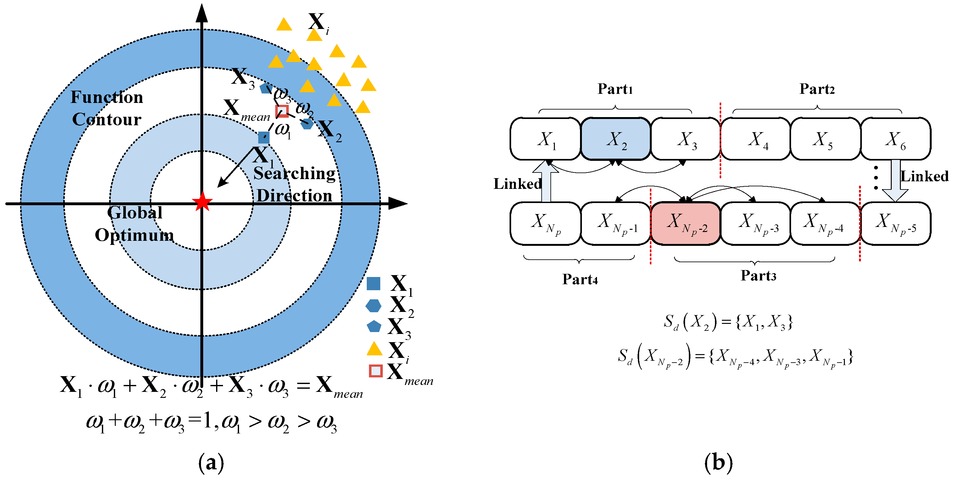
2.2. A Bionic Social Learning Strategy Pigeon-Inspired Optimization
2.3. Convergence Proof of the Bionic Social Learning Strategy Pigeon-Inspired Optimization
2.4. Complexity Analysis of the Bionic Social Learning Strategy Pigeon-Inspired Optimization
3. Experiment and Analysis of the Benchmark Functions Test
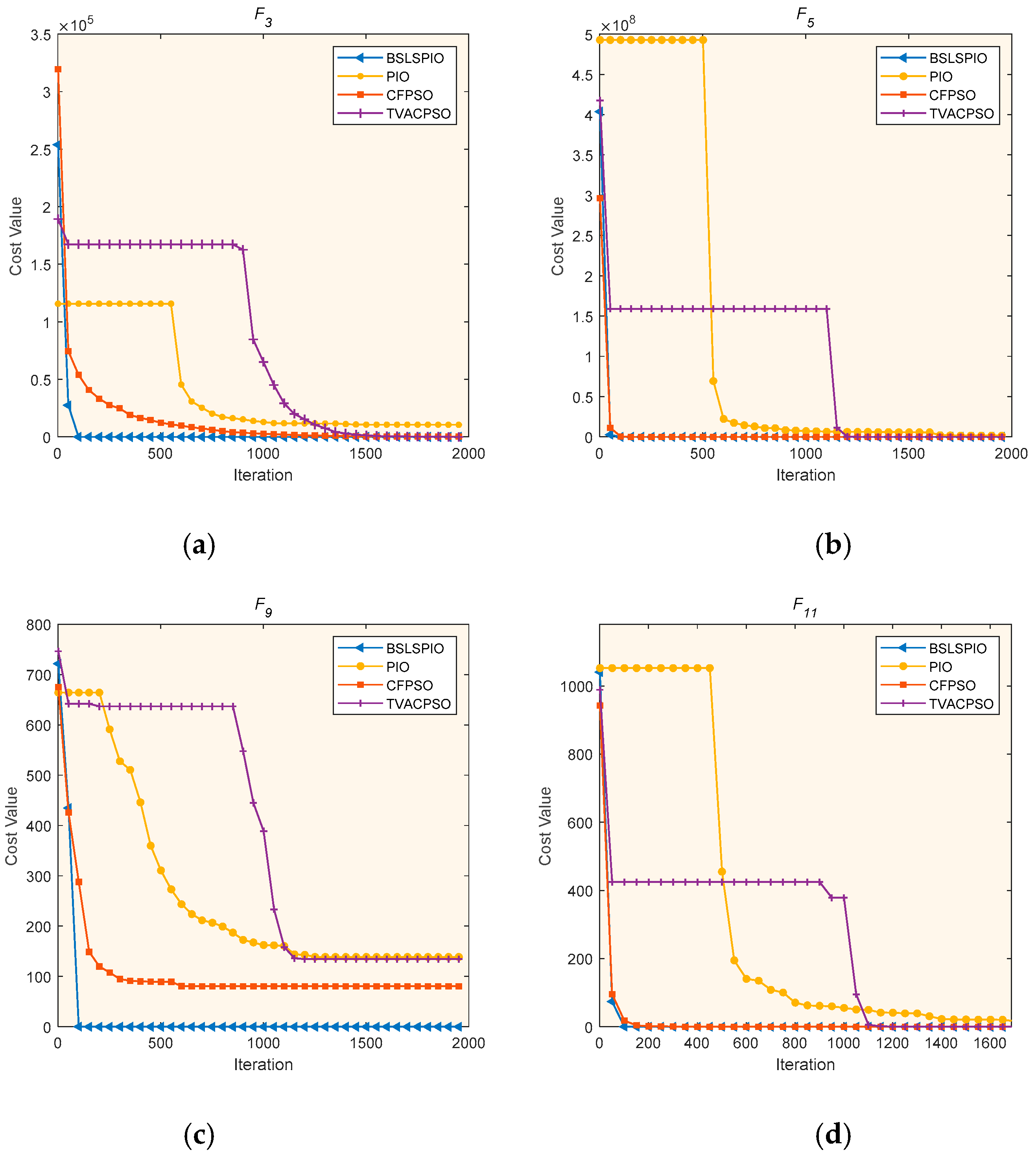
3.1. Performance on Uni-Modal and Multi-Modal Benchmark Functions
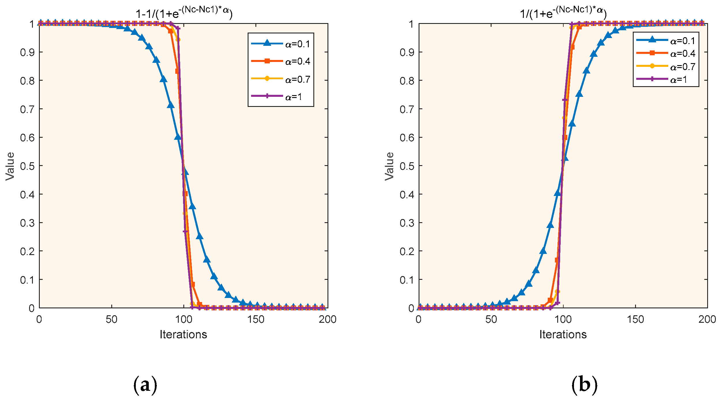
3.2. Influence of the Additional Parameters
4. UAV Path Planning with Cooperative Detection Using BSLSPIO
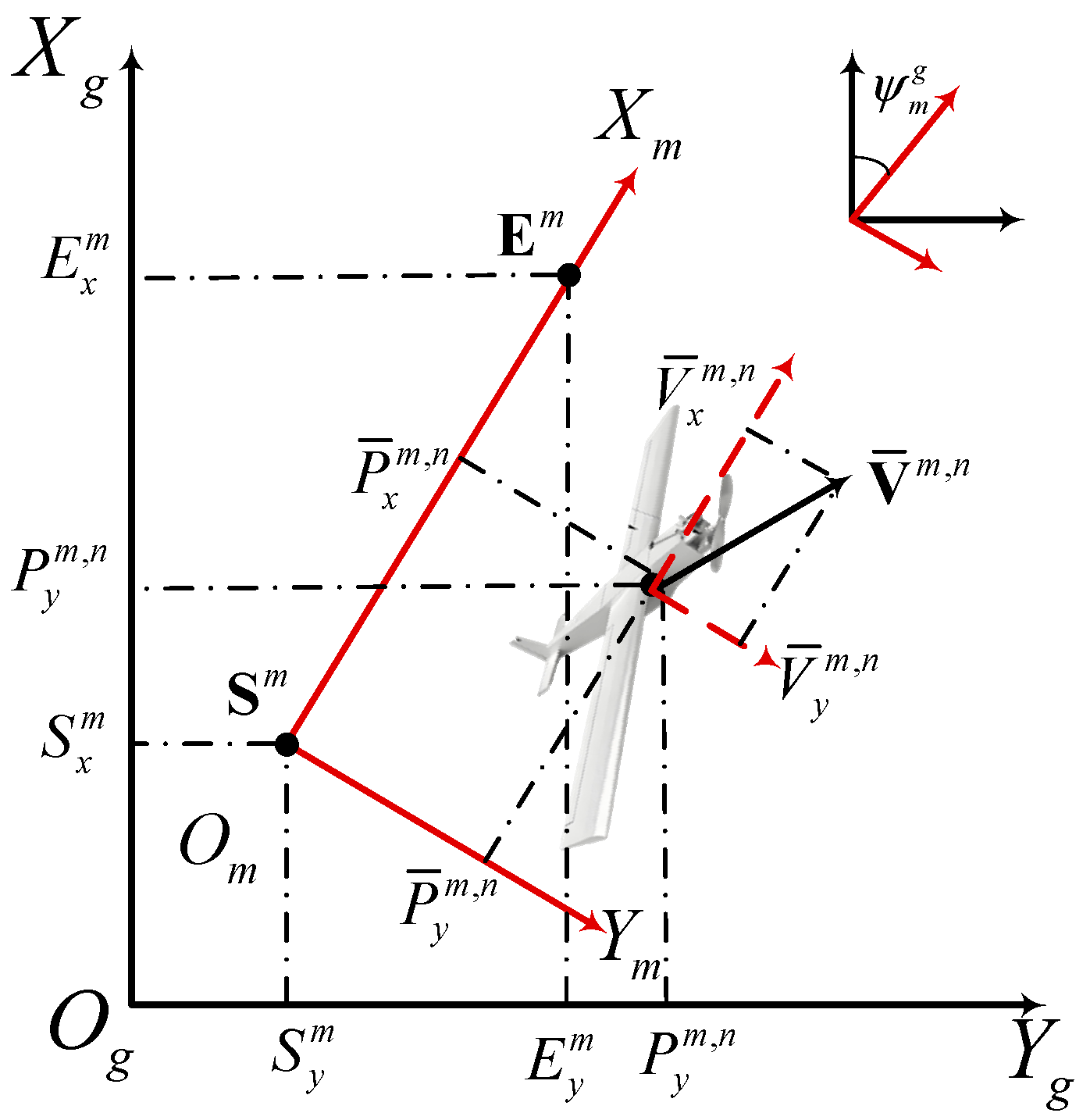
4.1. UAV Model
4.2. Path-Planning Models
- Models of the detection network:
- Detection modeling:
- Mountains cost:
- Coordination costs:
- Flight constraints:
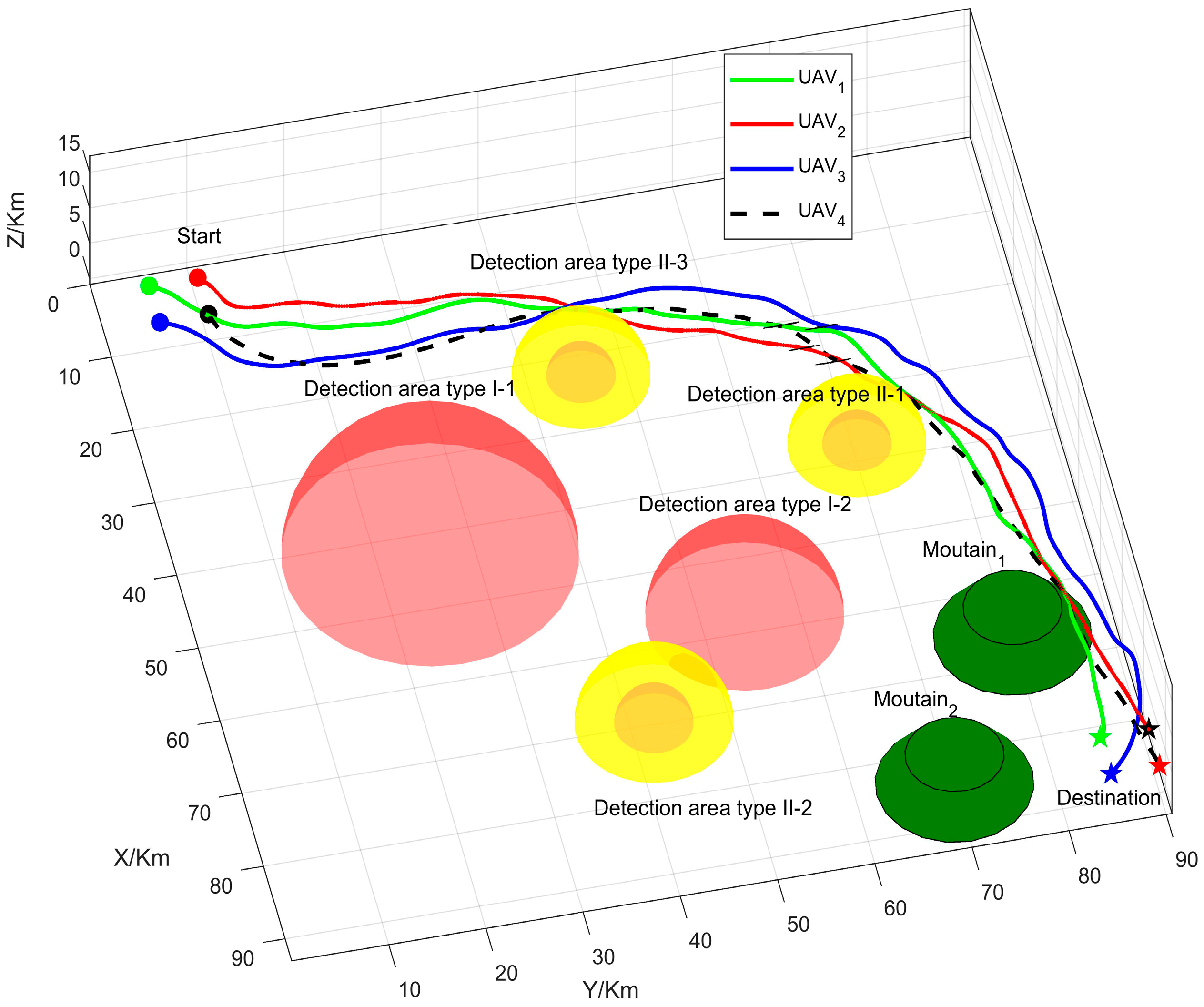
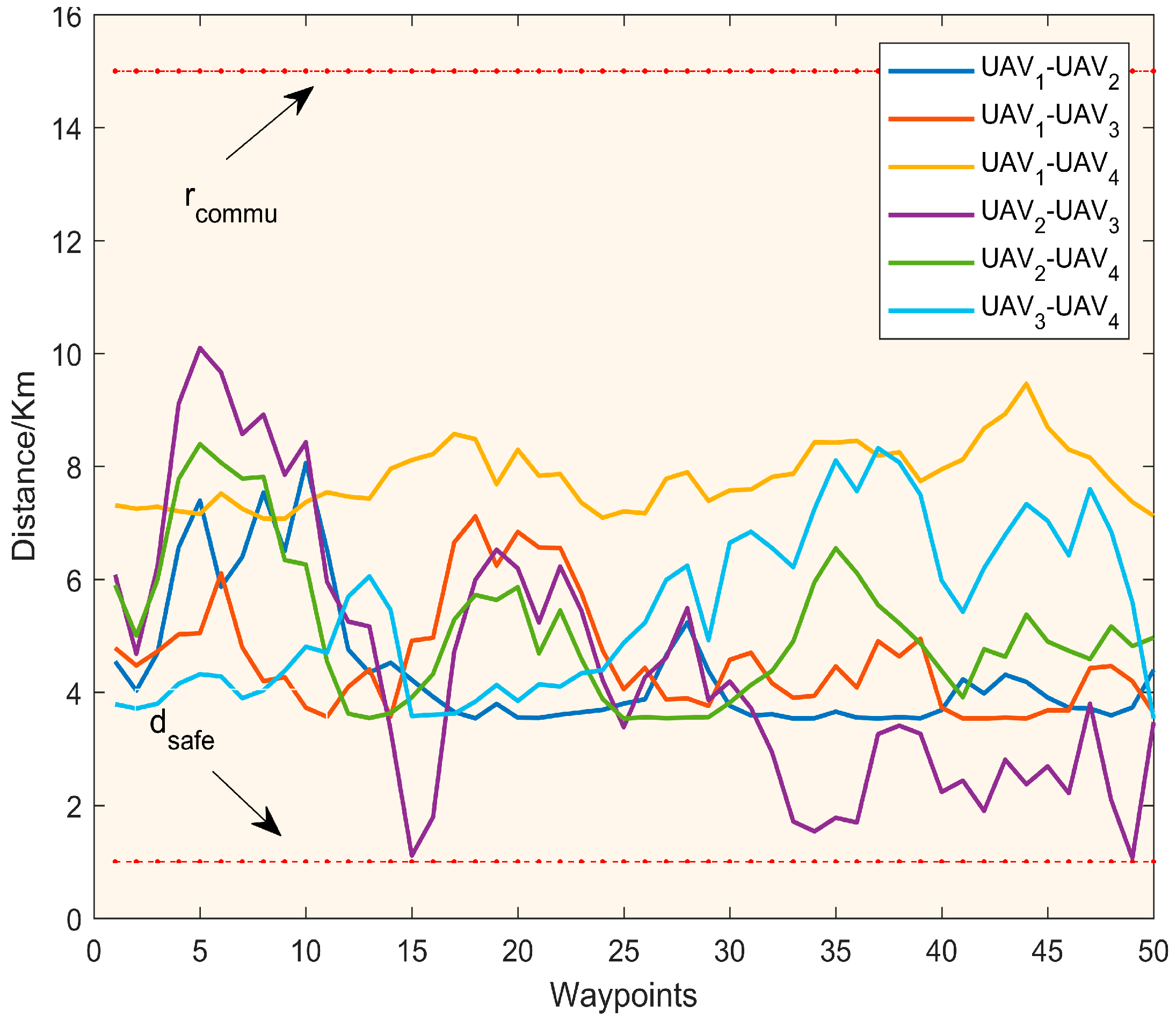
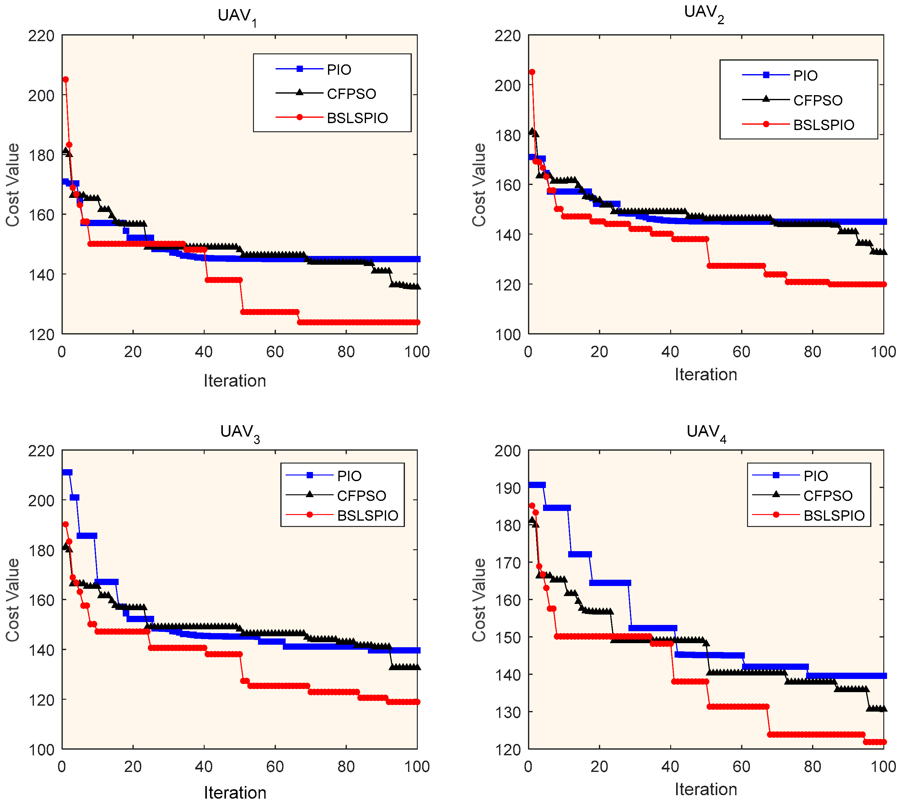
4.3. Simulation
5. Conclusions
Author Contributions
Funding
Institutional Review Board Statement
Informed Consent Statement
Data Availability Statement
Conflicts of Interest
References
- Chui, K.T.; Liu, R.W.; Zhao, M. Bio-inspired algorithms for cybersecurity—A review of the state-of-the-art and challenges. Int. J. Bio-Inspired Comput. 2024, 23, 1–15. [Google Scholar] [CrossRef]
- Chatterijee, Y.; Bourreau, E.; Rancic, M.J. Solving various NP-hard problems using exponentially fewer qubits on a quantum computer. Phys. Rev. A 2024, 109, 052441. [Google Scholar] [CrossRef]
- Das, S.; Suganthan, P.N. Differential evolution: A survey of the state-of-the-art. IEEE Trans. Evol. Comput. 2010, 15, 4–31. [Google Scholar] [CrossRef]
- Sivaraj, R. Novel Techniques for enhancing performance of genetic algorithms. AI Commun. 2016, 29, 545–546. [Google Scholar] [CrossRef]
- Yazdani, M.; Kabirifar, K.; Haghani, M. Optimising Post-disaster waste collection by a deep learning-enhanced differential evolution approach. Eng. Appl. Artif. Intell. 2024, 132, 107932. [Google Scholar] [CrossRef]
- Yang, Q.; Qiao, Z.Y.; Xu, P. Triple Competitive Differential evolution for global numerical optimization. Swarm Evol. Comput. 2024, 84, 101450. [Google Scholar] [CrossRef]
- Vargas, G.A.D.; Mosquera, D.J.; Trujillo, E.R. Optimization of topological reconfiguration in electric power systems using genetic algorithm and nonlinear programming with discontinuous derivatives. Electronics 2024, 13, 616. [Google Scholar] [CrossRef]
- Ballinas, E.; Montiel, O.; Martínez-Vargas, A. Hybrid quantum genetic algorithm with fuzzy adaptive rotation angle for efficient placement of unmanned aerial vehicles in natural disaster areas. Axioms 2024, 13, 48. [Google Scholar] [CrossRef]
- Chen, J.; Cai, H.; Wang, W. A new metaheuristic algorithm: Car tracking optimization algorithm. Soft Comput. 2018, 22, 3857–3878. [Google Scholar] [CrossRef]
- Wang, G.G.; Deb, S.; Coelho, L.D. Earthworm optimization algorithm: A bio-inspired metaheuristic algorithm for global optimization problems. Int. J. Bio-Inspired Comput. 2018, 12, 1–22. [Google Scholar] [CrossRef]
- Shareef, H.; Lbrahim, A.A.; Mutlag, A.H. Lightning search algorithm. Appl. Soft Comput. 2015, 36, 315–333. [Google Scholar] [CrossRef]
- Zhao, W.G.; Wang, L.Y.; Zhang, Z.X. Atom search optimization and its application to solve a hydrogeologic parameter estimation problem. Knowl.-Based Syst. 2019, 163, 283–304. [Google Scholar] [CrossRef]
- Oca, M.A.M.D.; Stutzle, T.; Enden, K.V.d. Incremental social learning in particle swarms. IEEE Trans. Syst. Man Cybern. Part B Cybern. 2011, 41, 368–384. [Google Scholar] [CrossRef] [PubMed]
- Abdesslem, L.; Zeyneb, B. A novel firefly algorithm based ant colony optimization for solving combinatorial optimization problems. Int. J. Comput. Sci. 2014, 11, 19–37. [Google Scholar]
- Snehlata, S.; Neetu, M.; Alexander, G. Artificial bee colony algorithm in data flow testing for optimal test suite generation. Int. J. Syst. Assur. Eng. 2020, 11, 340–349. [Google Scholar]
- Duan, H.B.; Qiao, P.X. Pigeon-inspired optimization: A new swarm intelligence optimizer for air robot path planning. Int. J. Intell. Comput. Cybern. 2014, 7, 24–37. [Google Scholar] [CrossRef]
- Liu, Y.; As’arry, A.; Hassan, M.K.; Hairuddin, A.A. Review of the grey wolf optimization algorithm: Variants and applications. Neural Comput. Appl. 2024, 36, 2713–2735. [Google Scholar] [CrossRef]
- Deng, L.; Liu, S. Deficiencies of the whale optimization algorithm and its validation method. Expert Syst. Appl. 2024, 237, 121544. [Google Scholar] [CrossRef]
- Yuan, G.S.; Duan, H.B. Extremum seeking control for UAV close formation flight via improved pigeon-inspired optimization. Sci. China Technol. Sci 2024, 67, 435–448. [Google Scholar] [CrossRef]
- Su, H.; Sun, Y.; Zeng, Z. Image segmentation model for vicinagearth security technology of unmanned aerial vehicle using improved pigeon-inspired optimization. Guid. Navig. Control 2024, 4, 2441002. [Google Scholar] [CrossRef]
- Jiang, Y.; Bai, T.; Wang, D. Coverage path planning of UAV based on linear programming-Fuzzy C-means with pigeon-inspired optimization. Drones 2024, 8, 50. [Google Scholar] [CrossRef]
- Liu, Y.; Wei, C.; Duan, H.B. Active disturbance rejection heading control of USV based on parameter tuning via an improved pigeon-inspired optimization. Trans. Inst. Meas. Control. 2024, 47, 1–24. [Google Scholar] [CrossRef]
- Xue, Q.; Duan, H.B. Robust attitude control for reusable launch vehicles based on fractional calculus and pigeon-inspired optimization. IEEE CAA J. Autom. Sin. 2017, 4, 89–97. [Google Scholar] [CrossRef]
- Duan, H.B.; Qiu, H.X. Advancements in pigeon-inspired optimization and its variants. Sci. China Inf. Sci. 2019, 62, 070201:1–070201:10. [Google Scholar] [CrossRef]
- Chen, S.J.; Duan, H.B. Fast image matching via multi-scale Gaussian mutation pigeon-inspired optimization for low cost quadrotor. Aircr. Eng. Aerosp. Technol. 2017, 89, 777–790. [Google Scholar] [CrossRef]
- Duan, H.B.; Yang, Z.Y. Large civil aircraft receding horizon control based on Cauthy mutation pigeon inspired optimization. Sci. Sin. Technol. 2018, 48, 277–288. [Google Scholar] [CrossRef]
- Sun, Y.B.; Duan, H.B.; Xian, N. Fractional-order controllers optimized via heterogeneous comprehensive learning pigeon-inspired optimization for autonomous aerial refueling hose-drogue system. Aerosp. Sci. Technol. 2018, 81, 1–13. [Google Scholar] [CrossRef]
- Li, S.Q.; Deng, Y.M. Quantum-entanglement pigeon-inspired optimization for unmanned aerial vehicle path planning. Aircr. Eng. Aerosp. Technol. 2019, 91, 171–181. [Google Scholar] [CrossRef]
- Xu, X.B.; Deng, Y.M. UAV power component-DC brushless motor design with merging adjacent-disturbances and integrated-dispatching pigeon-inspired optimization. IEEE Trans. Magn. 2018, 54, 1–7. [Google Scholar] [CrossRef]
- Zhang, D.F.; Duan, H.B. Social-class pigeon-inspired optimization and time stamp segmentation for multi-UAV cooperative path planning. Neurocomputing 2018, 313, 229–246. [Google Scholar] [CrossRef]
- Qiu, H.X.; Duan, H.B. A multi-objective pigeon-inspired optimization approach to UAV distributed flocking among obstacles. Inf. Sci. 2020, 509, 515–529. [Google Scholar] [CrossRef]
- Shan, X.; Wang, Y. Energy efficiency optimization for discrete workshop based on parametric knowledge pigeon swarm algorithm. J. Syst. Simul. 2017, 9, 2140–2148. [Google Scholar]
- Viadero-Monasterio, F.; Nguyen, A.T.; Lauber, J. Event-triggered robust path tracking control considering roll stability under network-induced delays for autonomous vehicles. IEEE Trans. Intell. Transp. Syst. 2023, 24, 14743–14756. [Google Scholar] [CrossRef]
- Sun, X.; Cai, C.; Shen, X. A new cloud model based human-machine cooperative path planning method. J. Intell. Robot. Syst. 2015, 79, 3–19. [Google Scholar] [CrossRef]
- Qin, P.; Liu, F.; Guo, Z. Hierarchical collision-free trajectory planning for autonomous vehicles based on improved artificial potential field method. Trans. Inst. Meas. Control 2024, 46, 799–812. [Google Scholar] [CrossRef]
- Bhattacharya, P.; Gavrilova, M. Roadmap-based path planning using the Voronoi diagram for a clearance-based shortest path. IEEE Robot. Autom. Mag. 2008, 15, 58–66. [Google Scholar] [CrossRef]
- Maini, P.; Sujit, P. Path planning for a UAV with kinematic constraints in the presence of polygonal obstacles. In Proceedings of the International Conference on Unmanned Aircraft Systems, Arlington, VA, USA, 4 July 2016; pp. 62–67. [Google Scholar]
- Gómez Arnaldo, C.; Zamarreño Suárez, M. Path Planning for unmanned aerial vehicles in complex environments. Drones 2024, 8, 288. [Google Scholar] [CrossRef]
- Hu, X.; Chen, L.; Tang, B. Dynamic path planning for autonomous driving on various roads with avoidance of static and moving obstacles. Mech. Syst. Signal Proc. 2018, 100, 482–500. [Google Scholar] [CrossRef]
- Fierrez, J.; Navarro, E. Adaptive morphological time stamp segmentation based on efficient global motion estimation. In Proceedings of the International Conference on Image Processing, Rochester, NY, USA, 22 September 2002; pp. 289–292. [Google Scholar]
- Whiten, A. Operant study of sun altitude and pigeon navigation. Nature 1972, 237, 405–406. [Google Scholar] [CrossRef]
- Dell’Ariccia, G.; Dell’Omo, G.; Wolfer, D.P. Flock flying improves pigeons’ homing: GPS track analysis of individual flyers versus small groups. Anim. Behav. 2008, 76, 1165–1172. [Google Scholar] [CrossRef]
- Heyes, C.; Ray, E.D.; Mitchell, C.J. Stimulus enhancement: Controls for social facilitation and local enhancement. Learn. Motiv. 2000, 31, 83–89. [Google Scholar] [CrossRef]
- Young, H.P. Innovation diffusion in heterogeneous populations: Contagion, social influence, and social learning. Am. Econ. Rev. 2009, 99, 1899–1924. [Google Scholar] [CrossRef]
- Bond, C.F.; Titus, L.J. Social facilitation: A meta-analysis of 241 studies. Psychol. Bull. 1983, 94, 265–292. [Google Scholar] [CrossRef]
- Zentall, T.R. Imitation in animals: Evidence, function, and mechanisms. Cybernet Syst. 2001, 32, 53–96. [Google Scholar] [CrossRef]
- Whiten, A. Primate culture and social learning. Cogn. Sci. 2000, 24, 477–508. [Google Scholar] [CrossRef]
- Naik, B.B.; Raju, C.P.; Rao, R.S. A constriction factor based particle swarm optimization for congestion management in transmission systems. Int. J. Electr. Eng. Inform. 2018, 10, 232–241. [Google Scholar] [CrossRef]
- Mohammadiivatloo, B.; Rabiee, A.; Soroudi, A. Iteration PSO with time varying acceleration coefficients for solving non-convex economic dispatch problems. Int. J. Electr. Power Energy Syst. 2012, 42, 508–516. [Google Scholar] [CrossRef]
- Zhan, Z.H.; Zhang, J.; Li, Y. Orthogonal learning particle swarm optimization. IEEE Trans. Evol. Comput. 2011, 15, 832–847. [Google Scholar] [CrossRef]

| Types | Name | Range | Optimum | |
| Uni-modal benchmark functions | F1 | Sphere model | [−100,100] N | 0 |
| F2 | Schwefel’s problem 2.22 | [−10,10] N | 0 | |
| F3 | Schwefel’s problem 1.2 | [−10,10] N | 0 | |
| F4 | Schwefel’s problem 2.21 | [−100,100] N | 0 | |
| F5 | Generalized Rosenbrock’s functions | [−30,30] N | 0 | |
| F6 | Step function | [−100,100] N | 0 | |
| F7 | Quartic function | [−1.28,1.28] N | 0 | |
| Multi-modal benchmark functions | F8 | Generalized Schwefel’s problem 2.26 | [−500,500] N | −418.9829 × N |
| F9 | Generalized Rastrigin’s function | [−5.12,5.12] N | 0 | |
| F10 | Ackley’s function | [−32,32] N | 0 | |
| F11 | Generalized Griewank function | [−600,600] N | 0 | |
| F12 | Generalized Penalized function 1 | [−50,50] N | 0 | |
| F13 | Generalized Penalized function 2 | [−50,50] N | 0 | |
| Algorithm | CFPSO | TVACPSO | PIO | BSLSPIO |
| Parameter settings |
| Methods | Avg | Std | Med | Rank | |
| F1 | CFPSO | 9.47 × 10⁻²⁷ | 2.97 × 10⁻²⁶ | 9.53 × 10⁻²⁸ | 2 |
| TVPSO | 2.80 × 10⁻¹³ | 7.75 × 10⁻¹³ | 5.33 × 10⁻¹⁴ | 3 | |
| PIO | 2136.0847 | 1123.6571 | 2101.5801 | 4 | |
| BSLSPIO | 0 | 0 | 0 | 1 | |
| F2 | CFPSO | 1.24 × 10⁻¹² | 4.85 × 10⁻¹² | 8.72 × 10⁻¹⁴ | 2 |
| TVPSO | 7.97 × 10⁻⁸ | 2.20 × 10⁻⁷ | 1.18 × 10⁻⁹ | 3 | |
| PIO | 27.3957 | 9.9191 | 25.6175 | 4 | |
| BSLSPIO | 0 | 0 | 0 | 1 | |
| F3 | CFPSO | 2010.4804 | 6091.3022 | 410.5686 | 3 |
| TVPSO | 94.4166 | 82.6071 | 67.0160 | 2 | |
| PIO | 29,839.9109 | 20,303.1877 | 27,833.7117 | 4 | |
| BSLSPIO | 0 | 0 | 0 | 1 | |
| F4 | CFPSO | 27.9293 | 10.7908 | 27.2225 | 4 |
| TVPSO | 15.4113 | 4.0431 | 14.9686 | 2 | |
| PIO | 23.9575 | 5.6872 | 23.8019 | 3 | |
| BSLSPIO | 0 | 0 | 0 | 1 | |
| F5 | CFPSO | 74.3672 | 54.3561 | 57.2061 | 2 |
| TVPSO | 92.0536 | 39.5895 | 96.0884 | 3 | |
| PIO | 1,279,313.4833 | 1,264,079.8109 | 888,139.5883 | 4 | |
| BSLSPIO | 48.8882 | 0.0205 | 48.8885 | 1 | |
| F6 | CFPSO | 4.8667 | 9.1151 | 1.5000 | 2 |
| TVPSO | 29.3667 | 21.9819 | 22.5000 | 3 | |
| PIO | 14,317.9333 | 4141.05242 | 13,939.5000 | 4 | |
| BSLSPIO | 0 | 0 | 0 | 1 | |
| F7 | CFPSO | 0.0127 | 0.0043 | 0.0122 | 2 |
| TVPSO | 0.0841 | 0.0350 | 0.0763 | 3 | |
| PIO | 13.1480 | 5.25569 | 11.2427 | 4 | |
| BSLSPIO | 3.80 × 10⁻⁶ | 3.54 × 10⁻⁶ | 2.48 × 10⁻⁶ | 1 | |
| F8 | CFPSO | −14,651.8092 | 533.6465 | −14,661.5504 | 1 |
| TVPSO | −13,690.6476 | 722.5480 | −13,615.4023 | 2 | |
| PIO | −11,174.7664 | 1737.2869 | −11,144.1739 | 3 | |
| BSLSPIO | −4788.7586 | 485.1123 | −4725.8601 | 4 | |
| F9 | CFPSO | 108.11866 | 20.3810 | 103.9730 | 2 |
| TVPSO | 113.8231 | 20.5732 | 113.4251 | 3 | |
| PIO | 162.6306 | 21.3486 | 160.5944 | 4 | |
| BSLSPIO | 0 | 0 | 0 | 1 | |
| F10 | CFPSO | 1.1372 | 0.8397 | 1.3220 | 2 |
| TVPSO | 3.4449 | 1.5962 | 2.9647 | 3 | |
| PIO | 14.7115 | 2.0469 | 14.7623 | 4 | |
| BSLSPIO | 0 | 0 | 0 | 1 | |
| F11 | CFPSO | 0.0054 | 0.0095 | 0 | 2 |
| TVPSO | 0.0506 | 0.1492 | 3.0498 × 10⁻¹³ | 3 | |
| PIO | 21.0374 | 11.7086 | 16.7073 | 4 | |
| BSLSPIO | 0 | 0 | 0 | 1 | |
| F12 | CFPSO | 0.1832 | 0.3246 | 0.0311 | 1 |
| TVPSO | 0.3832 | 0.5081 | 0.0978 | 2 | |
| PIO | 246,661.6902 | 1,271,510.9285 | 14.9824 | 4 | |
| BSLSPIO | 0.8017 | 0.0821 | 0.8004 | 3 | |
| F13 | CFPSO | 0.0066 | 0.0114 | 1.9134 × 10⁻²³ | 1 |
| TVPSO | 0.2302 | 0.8032 | 0.0110 | 2 | |
| PIO | 589,203.9899 | 122,0421.8138 | 6302.2066 | 4 | |
| BSLSPIO | 4.9778 | 0.0294 | 4.9886 | 3 |
| Uni-Modal Benchmark Functions | |||||||
| F1 | F2 | F3 | F4 | F5 | F6 | F7 | |
| Avg | 0 | 0 | 0 | 0 | 998.8497 | 0 | 2.16 × 10⁻⁶ |
| Std | 0 | 0 | 0 | 0 | 0.0269 | 0 | 2.36 × 10⁻⁶ |
| Med | 0 | 0 | 0 | 0 | 998.8519 | 0 | 1.28 × 10⁻⁶ |
| Multi-Modal Benchmark Functions | |||||||
| F8 | F9 | F10 | F11 | F12 | F13 | ||
| Avg | −22,604.3559 | 0 | 0 | 0 | 1.1482 | 99.9825 | |
| Std | 2113.57601 | 0 | 0 | 0 | 0.0077 | 0.0050 | |
| Med | −22,364.7032 | 0 | 0 | 0 | 1.1477 | 99.9835 | |
| Start Position (km) | End Position (km) | |||
| UAVs States | UAV1 | (5, 5, 3) | (85, 85, 3) | |
| UAV2 | (5, 10, 3) | (85, 90, 3) | ||
| UAV3 | (10, 5, 3) | (90, 85, 3) | ||
| UAV4 | (10, 10, 3) | (90, 90, 3) | ||
| Position (km) | Radius (km) | Communication Range (km) | ||
| Detection Units | type I-1 | (45, 25) | 15 | 60 |
| type I-2 | (60, 54) | 10 | 50 | |
| type II-1 | (40, 70) | 7 | 30 | |
| type II-2 | (72, 42) | 8 | 30 | |
| type II-3 | (25, 45) | 7 | 30 | |
| Position (km) | (km) | Height (m) | ||
| Mountains | Mountain1 | (67, 80) | (8, 5) | 60 |
| Mountain2 | (85, 70) | (8, 5) | 50 | |
| 1 | 300 | |||
| Constraints | 400 km/h | 300 km/h | ||
| 1.2274 km | 1 h | |||
| 0.0066 h | 0 h | |||
| 0.33 h | 0.9383 rad | |||
| 342.85 km/h | (−233.90, 233.90) km/h | |||
| 1 km | 15 km | |||
| 50 | ||||
| Other Parameters | 1.01 | 1.25 × 10⁻¹⁸ | ||
| 2.4637 | 0.05 | |||
| 0.8 | 0.6 | |||
Disclaimer/Publisher’s Note: The statements, opinions and data contained in all publications are solely those of the individual author(s) and contributor(s) and not of MDPI and/or the editor(s). MDPI and/or the editor(s) disclaim responsibility for any injury to people or property resulting from any ideas, methods, instructions or products referred to in the content. |
© 2025 by the authors. Licensee MDPI, Basel, Switzerland. This article is an open access article distributed under the terms and conditions of the Creative Commons Attribution (CC BY) license (https://creativecommons.org/licenses/by/4.0/).
Share and Cite
Shen, Y.; Liu, X.; Ma, X.; Du, H.; Xin, L. A Bionic Social Learning Strategy Pigeon-Inspired Optimization for Multi-Unmanned Aerial Vehicle Cooperative Path Planning. Appl. Sci. 2025, 15, 910. https://doi.org/10.3390/app15020910
Shen Y, Liu X, Ma X, Du H, Xin L. A Bionic Social Learning Strategy Pigeon-Inspired Optimization for Multi-Unmanned Aerial Vehicle Cooperative Path Planning. Applied Sciences. 2025; 15(2):910. https://doi.org/10.3390/app15020910
Chicago/Turabian StyleShen, Yankai, Xinan Liu, Xiao Ma, Hong Du, and Long Xin. 2025. "A Bionic Social Learning Strategy Pigeon-Inspired Optimization for Multi-Unmanned Aerial Vehicle Cooperative Path Planning" Applied Sciences 15, no. 2: 910. https://doi.org/10.3390/app15020910
APA StyleShen, Y., Liu, X., Ma, X., Du, H., & Xin, L. (2025). A Bionic Social Learning Strategy Pigeon-Inspired Optimization for Multi-Unmanned Aerial Vehicle Cooperative Path Planning. Applied Sciences, 15(2), 910. https://doi.org/10.3390/app15020910