Sidewall Roughness Measurement and Bearing Performance Simulation of Rock-Socketed Piles Based on Laser Scanning Point Cloud

Abstract

Rock-socketed piles are commonly used in pile foundations for large buildings because of their excellent load-bearing characteristics. The roughness of the pile–rock interface affects the load transfer and the ultimate side resistance of the pile. In this work, a laser radar system is developed to measure the surface roughness of a dry bored pile and the shape of the borehole, and a three-dimensional model of the borehole is reconstructed based on the laser point cloud. The 3D surface model was used to extract the vertical contour lines in different directions and thus calculate the roughness of the pile. A numerical simulation of the real measured 3D model using FLAC3D is presented. A borehole of a real rock-socketed pile was measured and simulated. The results show that, although the working load is carried by both the side and base resistances, the former plays a major role. The slow-varying load-settlement curve indicates that the pile has a superior load–bearing capacity, and the maximum allowable settlement should be considered in the application. The simulations, using the actual piles tested, produced a more realistic load response and were able to predict the load-bearing performance of the piles more accurately. Furthermore, this approach offers a reference for the design of rock-socketed piles.

1. Introduction

Rock-socketed piles are a prevalent form of pile foundation utilized in underground bedrock to transfer structural loads of large buildings. They exhibit high bearing performance, low settlement, and allow for the full exploitation of the structural strength of the pile body and the surrounding rock mass. The bearing capacity of rock-socketed piles is attributable primarily to two factors: side frictional resistance and pile base resistance. Among these factors, the side resistance shaft resistance is considered the dominant factor under common working loads [1,2,3]. The development of side resistance is influenced primarily by the shear stress at the pile–rock contact interface, which is largely contingent on the material strength of the pile and the rock body, as well as the interface morphology [4]. Additionally, extensive laboratory experiments and field observations have demonstrated that the roughness of a hole wall strongly affects the bearing capacity of rock-socketed piles.

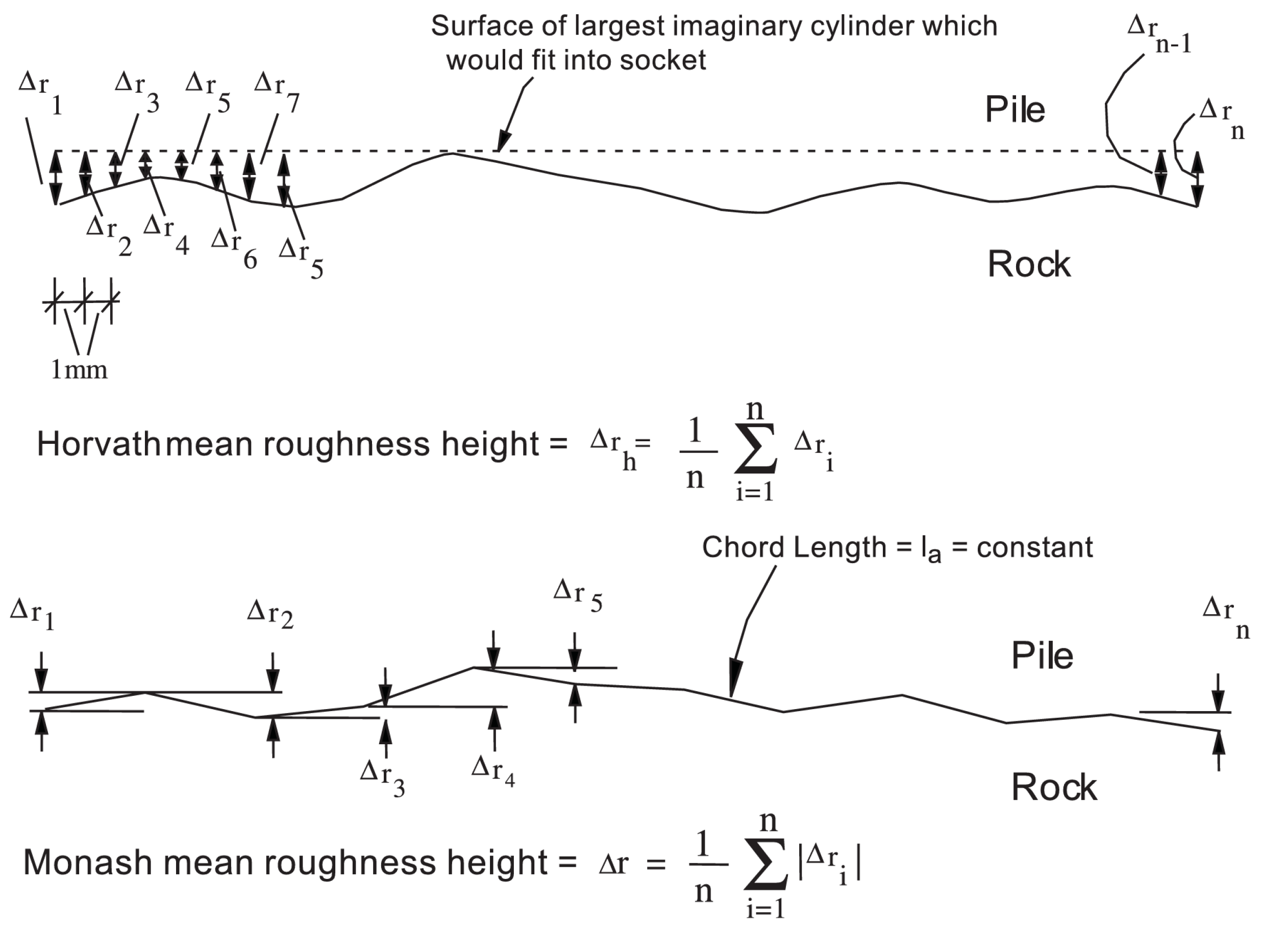
In a previous study, Pells et al. [5] examined the roughness of the sleeves formed via various drilling techniques in Sydney sandstone. They classified the hole wall roughness into four grades on the basis of the size of the concavity and convexity of the inner wall of the borehole. Subsequently, Rowe et al. [6], Williams et al. [4], Horvath et al. [7] investigated the correlation and influencing factors between the side resistance and roughness from different perspectives. Rowe et al. proposed a relationship between the ultimate side friction resistance and hole wall roughness, and Williams et al. noted that the degree of roughness was influenced by the rock type, the drilling method employed, and the drilling speed. Furthermore, Horvath et al. proposed a factor, $RF$, for the quantitative characterization of roughness, which accounts for the socket length, hole radius, and undulation of the sidewall. Seidel et al. [8] proposed a shaft resistance coefficient SRC that can describe the side resistance–settlement relationship by idealizing the undulating rock surface as multiple short lines of constant length, and assuming that the bump heights are approximated as Gaussian distributions, as shown in Figure 1.

The aforementioned studies were typically founded upon experimental and idealized analyses. With the swift advancements in computer technology and numerical modeling, the ability to construct intricate pile–rock models, and rapidly solve and compute them has become possible. Numerical simulations, including the finite element method (FEM) [9,10,11,12], discrete element method (FDM) [13], and boundary element method (BEM), have been employed by numerous researchers to examine the side resistance [14,15,16] and shear response of rock-socketed piles [17,18,19,20]. For example, Emirler et al. [21] utilized a finite element approach to investigate the influence of pile surface roughness on the pile load-carrying capacity and elucidate the associated damage mechanism. Similarly, Gutiérrez-Ch et al. [15] conducted load tests using a numerical discrete element model of a rock-socketed pile to analyze the effects of different roughnesses on the settlement response and lateral shear capacity. Jiang et al. [22] solved the load–displacement curves using the finite difference method and assumed that the contact interface was circular and wavy, with the goal of considering the effect of roughness on the bearing capacity.

The roughness data employed in the aforementioned methods is typically measured by a mechanical profilometer [23]. The amount of data measured by profilometers is relatively small, and the accuracy is relatively low. Liu et al. [24] utilized an umbrella-shaped aperture gauge to measure the aperture of bored piles and designed the roughness of the pile bodies based on the aperture. Nevertheless, in reality, the aperture cannot completely reflect the roughness of the hole wall. Subsequently, ultrasound was employed to measure the shape of the boreholes [25]. Since ultrasound utilizes the slurry to transmit sound waves and thereby obtain the positional information of the hole wall, its measurement accuracy is highly influenced by the properties of the slurry. When the density of the slurry is non-uniform, the measured roughness of the hole wall will become unreliable. Conversely, the more advanced laser method has gained widespread acceptance in the field of measurement. The laser’s independence from mud propagation enables it to measure the dry hole and circumvent the inaccuracy inherent in wave velocity calculation, arising from disparate mud properties. The laser sensor is smaller in size, with higher measurement accuracy and efficiency, and is more suitable for the detection of dry boreholes in pile foundations. However, there is a lack of laser equipment available for the detection of dry boreholes in pile foundations.

Owing to the dearth of real and sufficient hole wall roughness data, these previous methods typically employ approximate empirical formulas to calculate the roughness, or utilize a limited amount of local data to represent the overall roughness. Moreover, equivalent roughness factors are commonly applied in simulations, whereas direct numerical simulations utilizing actual three-dimensional models are seldom considered. In fact, sparse data with large errors may weaken the confidence of the simulation results, leading to distortions in the shaft resistance and load curves. Accordingly, a 3D laser scanning-based borehole roughness measurement instrument was developed for the purpose of accurately measuring the point cloud of the borehole wall and extracting the surface roughness. The point cloud is employed to reconstruct the surface model of the borehole in three dimensions, and subsequently, the roughness and morphological undulations of the borehole wall are extracted from the three-dimensional model. Additionally, the reconstructed 3D model was imported into FLAC3D for simulation of the ballast, allowing for the calculation of the bearing response of the rock-socketed pile and the proportion of side resistance to the total bearing capacity. The three-dimensional numerical simulation provides a comprehensive and effective response to the bearing characteristics and settlement characteristics of the pile foundation. Finally, the extracted roughness is introduced into the approximate empirical formula to calculate the theoretical axial side resistance of the pile, thereby verifying the validity of the results of the three-dimensional numerical simulation.

2. Method

2.1. Borehole Laser Scanning System

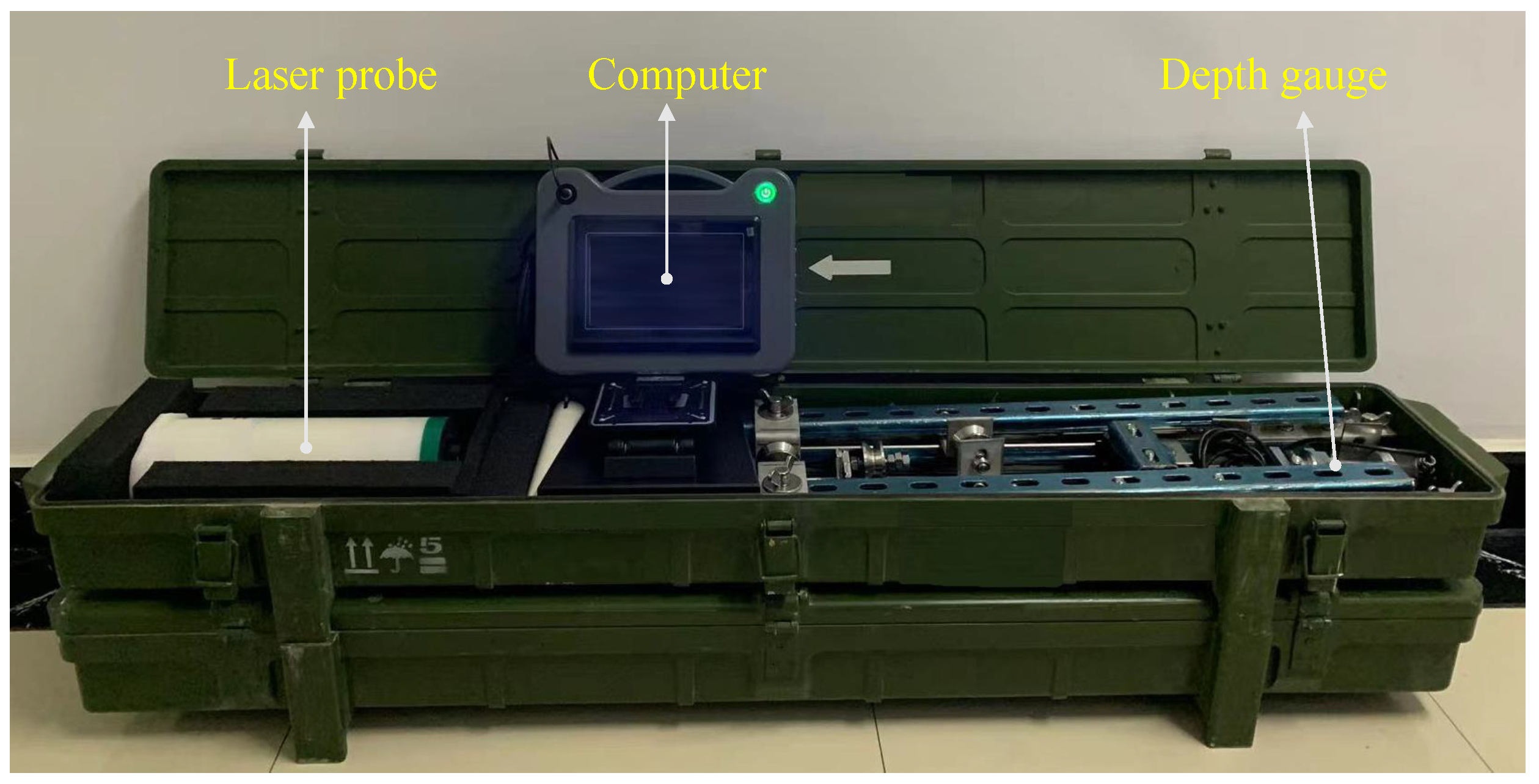
To access the surface morphology of boreholes for rock-socketed piles in situ, a LiDAR-based roughness measurement system was developed. The system utilizes the flight time of the laser to range, enabling the rapid acquisition of the surface morphology of the measured borehole. The system hardware comprises a laser probe, depth gauge, stabilizer, computer, CNC winch, and the necessary power supply and data transmission cables. A photograph of the main components of the laser system is shown in Figure 2. The system is capable of automatically measuring dry boreholes of varying diameters and depths, with a minimum diameter of 0.1 m, and can complete the sizing process with high precision and efficiency.

In the field, the devices are positioned as illustrated in Figure 3, with a computer utilized to oversee the entirety of the measurement process. The CNC winch is employed to lower and elevate the LiDAR in a vertical trajectory, and the sampling density of the drilling point cloud can be regulated by modulating the lowering velocity. A depth gauge is affixed to the winch and linked to the LiDAR via a cable, enabling real-time recording of the depth at which the LiDAR was situated. The LiDAR continuously emits laser beams and receives reflected signals from the borehole wall while descending at a constant speed. It also continuously rotates to scan the borehole wall step by step, recording and transmitting the time difference and rotation angle in real time. A corrector is employed to mitigate the impact of laser vibration on the measurement accuracy.

The above raw data were summarized in a computer for processing to obtain the 3D point cloud data of the borehole. First, the ranging and angular values recorded by the laser probe were used to calculate the 2D polar coordinate positions of the points on the rock surface within the borehole, and this polar coordinate system, with the center of the laser sensor at the time of the measurement as the origin, represents the cross-section of the borehole at different depths. The depth data were subsequently introduced to transform the 2D coordinates of the points into the 3D coordinate system in which the entire borehole is located. This conversion process is shown in Equation (1),

$${\mathrm{P}}_{\left(x_i,y_i\right)}=\left({\displaystyle \frac{1}{2}}ct·cos\alpha ,{\displaystyle \frac{1}{2}}ct·sin\alpha \right)\stackrel{+D}{\to }{P}_{\left(x_i,y_i,z_i\right)}=\left({\displaystyle \frac{1}{2}}ct·cos\alpha ,{\displaystyle \frac{1}{2}}ct·sin\alpha ,d\right)$$

(1)

where c is the speed of light, t and $\alpha$ is the time and angular values recorded by the laser probe, respectively.

2.2. Reconstruction of Borehole Models

The raw point clouds acquired via laser scanning are typically of inferior quality and contain noise and outliers resulting from the subsurface environment, equipment errors, and other factors. To reconstruct a superior mesh model, these data must undergo filtering to remove these artifacts. As outliers are characterized by a sparse distribution, and are situated at a considerable distance from the main body of the point cloud, they can be effectively removed through the utilization of statistical filtering. Statistical filtering is a method of removing outliers on the basis of the density of the point cloud. The fundamental premise is to initially traverse and calculate the distance between each point and its K nearest neighbors, which satisfies a Gaussian distribution. The distances of each point are subsequently compared with the population mean and variance, with points outside the n-fold variance considered outliers. Additionally, noise is typically Gaussian distributed near the hole wall and is eliminated through bilateral filtering. Compared with the commonly utilized Gaussian filtering, nonlinear bilateral filtering is capable of more effectively preserving the edge features of the point cloud while simultaneously facilitating superior handling of Gaussian noise. This prevents the loss of the roughness of the whole wall due to excessive smoothing.

Given the discontinuous nature of the 3D point cloud, it is not possible to extract and numerically simulate the roughness of the continuous hole wall. Accordingly, this paper presents a methodology for extracting a continuous surface model of a borehole from an unorganized point cloud. There are numerous surface reconstruction algorithms that are based on point clouds. In this paper, we utilize the Delaunay triangulation algorithm, which preserves the original position of the points. Unlike other algorithms, this approach does not alter the position of the point cloud, ensuring that the dissection results are unique and accurately reflect the true geometric features of the borehole. Additionally, it avoids smoothing the surface of the model, thus preventing any adverse effects on the roughness of the borehole surface.

2.3. Roughness Measurement and Characterization

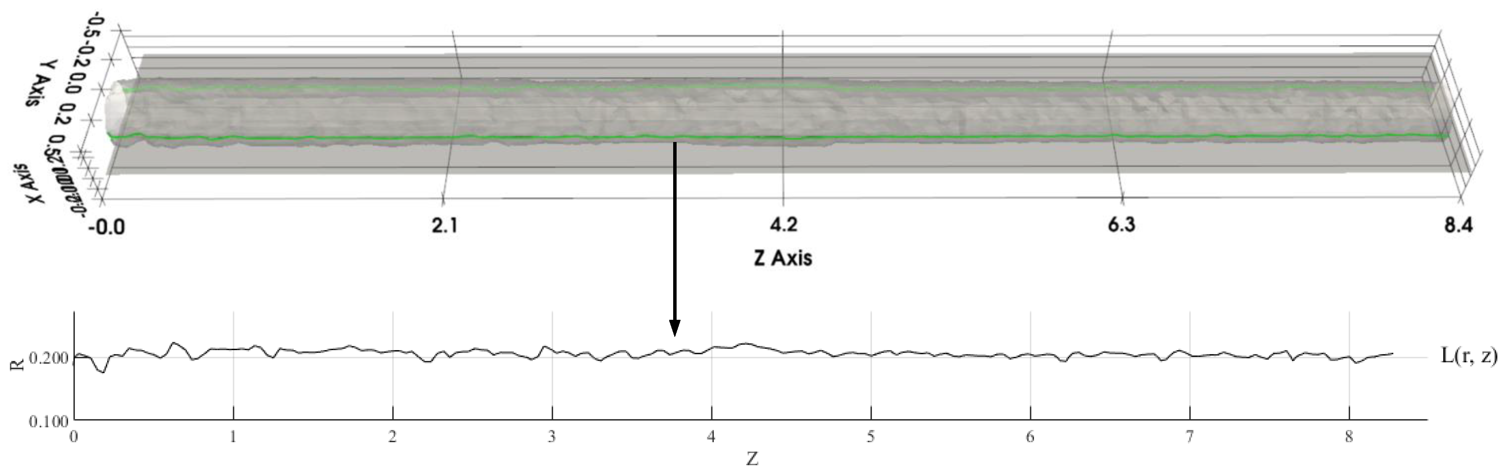
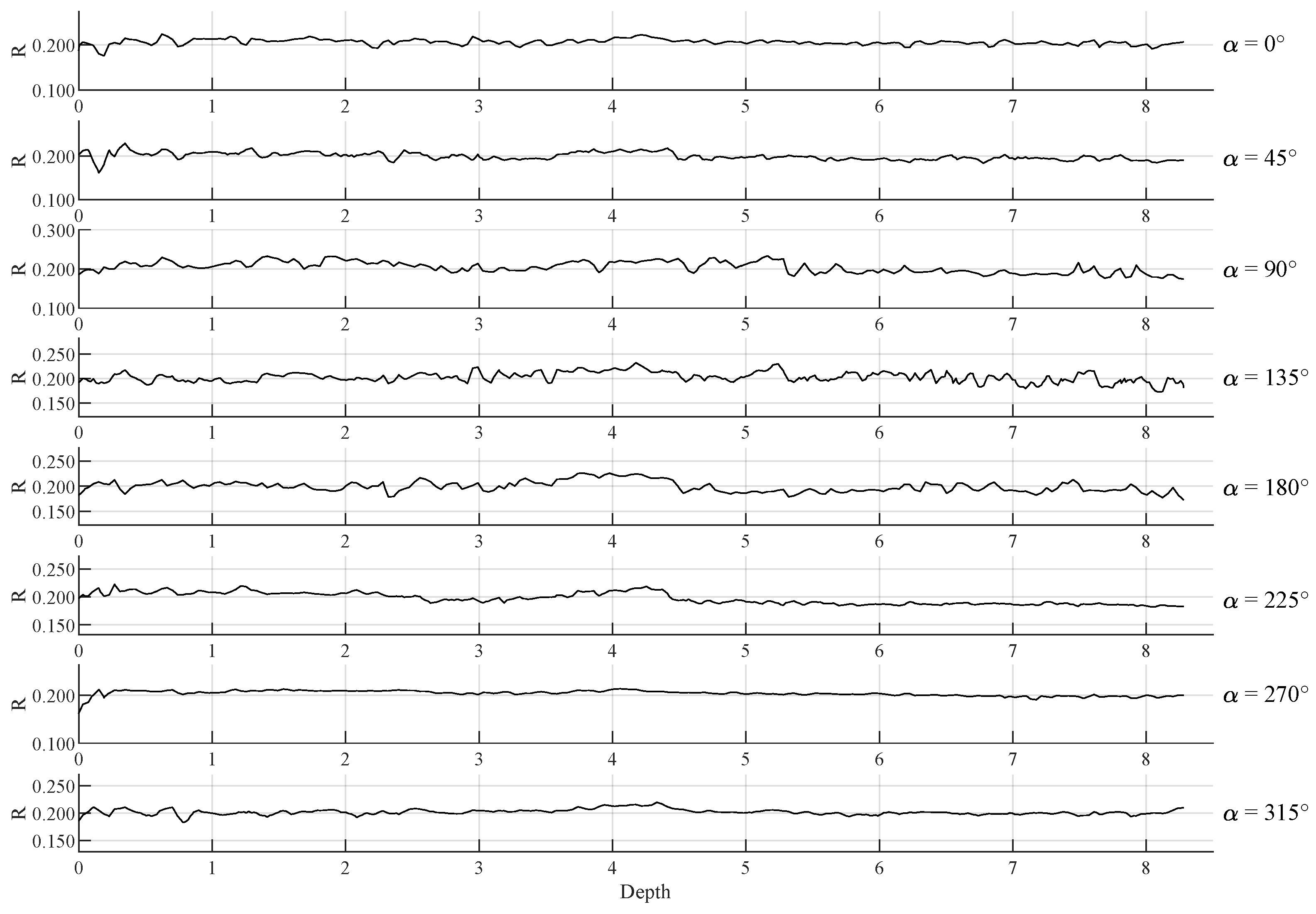
When the vertical bearing capacity of rock-socketed piles is considered, the roughness of the borehole wall in the vertical direction is the main concern because the shear action mainly occurs in the vertical direction. The reconstructed 3D mesh model is vertically dissected to extract the contour lines of the borehole in different orientations. Taking the central axis of the borehole as the center axis, the borehole is sectioned using planes with different angles, and the intersection lines between the planes and the surface model are the vertical contour lines of the corresponding angles, as shown in Figure 4. Moreover, since the surface model is continuous in three-dimensional space, it is theoretically possible to intercept countless contour lines with different orientations, thus obtaining the complete 360° roughness information of the drill hole.

To characterize the roughness of the drilled hole contour lines, the roughness factor $RF$ proposed by Horvath is introduced. $RF$ is calculated according to Equation (2), where r is the average roughness height, $r_h$ is the radius of the drilled hole, $L_t$ is the length of the bumpy and undulating contour lines, and $L_s$ is the nominal hole depth. Given that the extracted contour lines are in 3D coordinates, a conversion to radius undulations along the depth direction is undertaken in accordance with the specifications set forth in Equation (3).

$$RF={\displaystyle \frac{\Delta r_h}{r}}{\displaystyle \frac{L_t}{L_s}}$$

(2)

$$L\left(r,z\right)=\left(\sqrt{x_i^2+y_i^2},z_i\right)$$

(3)

2.4. FLAC3D Modelling

This section outlines the methodology for utilizing the reconstructed 3D surface model and FLAC3D for numerical simulation, with the objective of determining the ballast response of the rock-socketed pile. Given that the filled concrete can better accommodate the shape of the borehole, and that the shape of the pile is primarily determined by that of the borehole, it is possible to replace the geometric model of the pile with the reconstructed borehole model. In the traditional use of FLAC3D for load simulation, the lack of realistic pile geometry, and the difficulty of modeling many uneven microelements in detail, have led to the use of smooth cylinders endowed with certain shear parameters instead of real piles. However, this approach fails to account for the varying directions and magnitudes of the undulations, and the accuracy of the results is contingent upon the precise specification of the roughness and friction parameters. In this regard, this paper employs a 3D mesh model based on actual measurements for numerical simulation, which increases the model preprocessing procedure and the complexity of solving the calculation but reduces the error introduced by parameter estimation. The simulation results are more accurate, and more comprehensively reflect the bearing performance of the pile foundation.

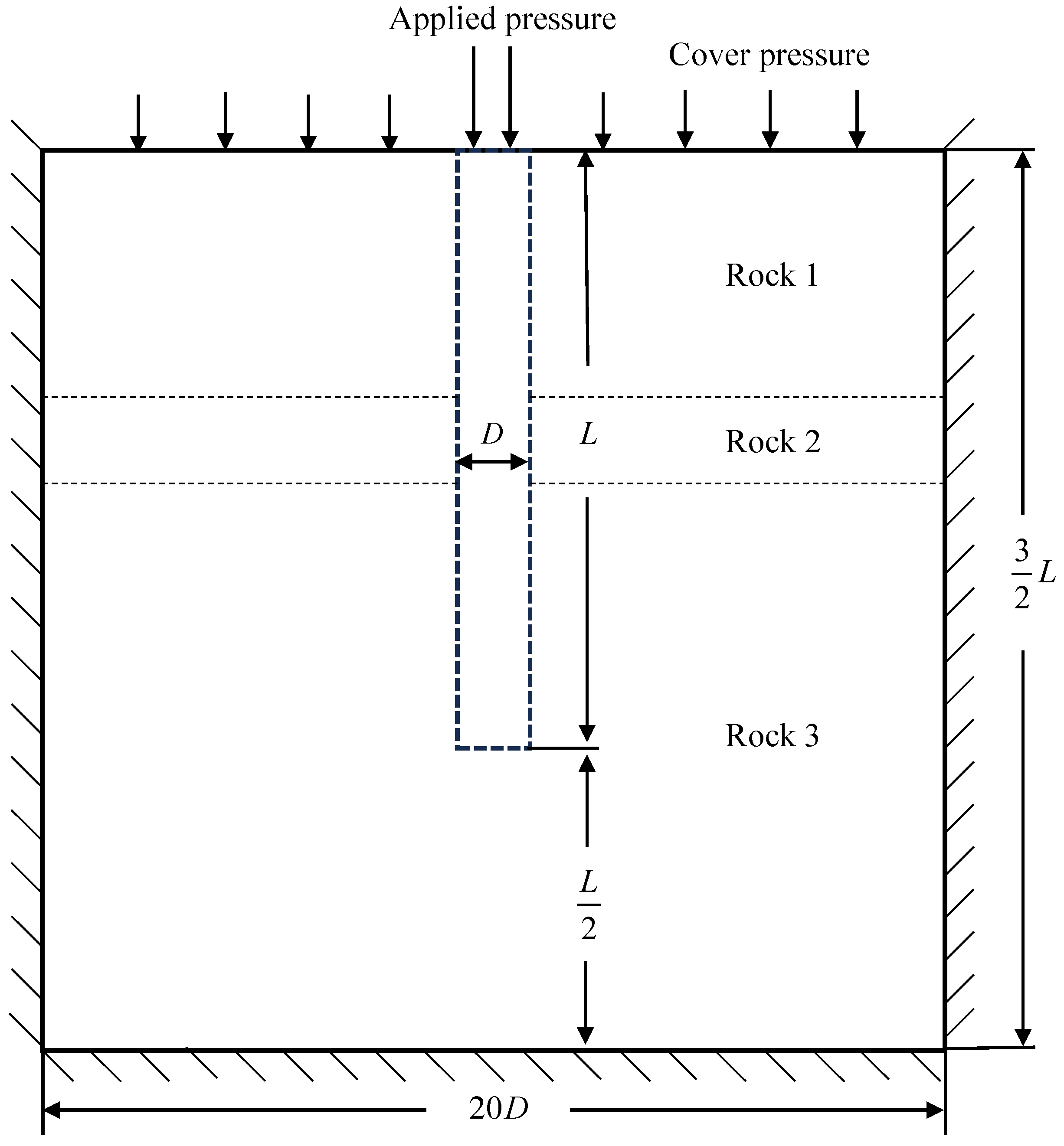
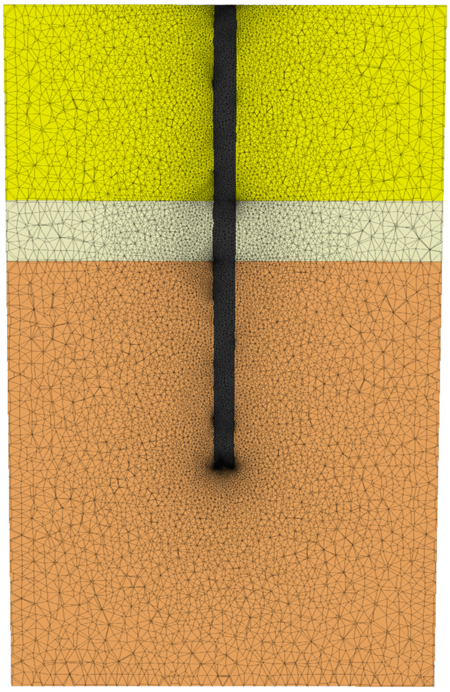
The surface model, reconstructed from the point cloud, contains a multitude of complex triangular meshes of varying dimensions. This method lacks the upper and lower surfaces of the unmeasured pile, which cannot be directly imported into FLAC3D for simulation. Accordingly, a model preprocessing stage was incorporated into the workflow to ensure the construction of a comprehensive and accurate pile–rock model. In this work, the top and bottom surfaces of the reconstructed model were complemented using Rhinoceros 8 modeling software, thereby forming a closed pile model. The pile body is subsequently positioned at the coordinate center, and several different stratigraphic models are constructed around the pile body in accordance with the actual conditions of the strata. The overall dimensions of the stratigraphic models are illustrated in Figure 5. They have a length and width of $20D$ and a height of ${\displaystyle \frac{3}{2}}L$, where D and L are the diameter and length of the pile, respectively. This range is sufficient to avoid the boundary effect of the geotechnical soil on the results, as previously discussed in reference [26].

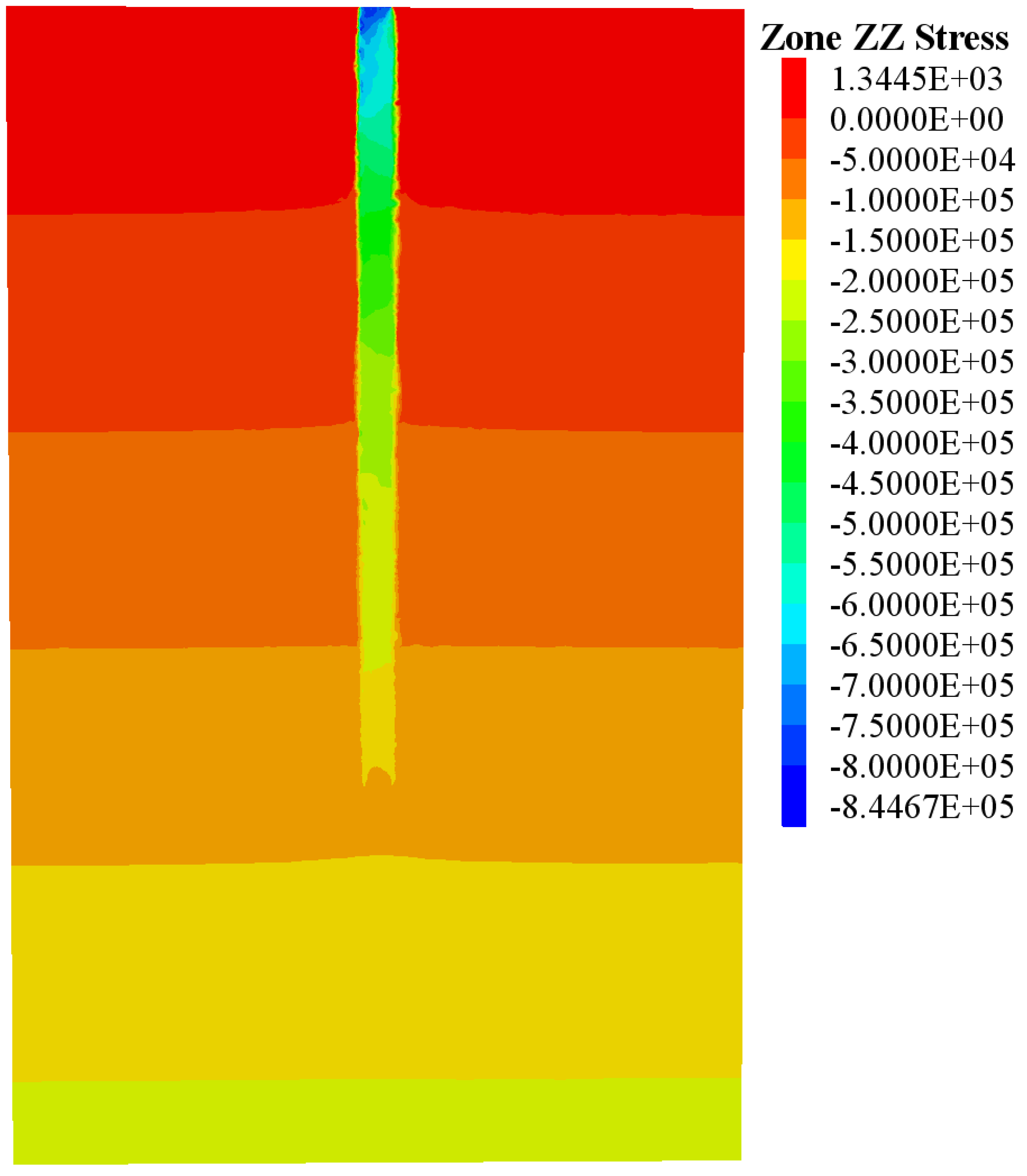
The pile–rock model is imported into FLAC3D for simulation, and the load test can be divided into 3 steps. In Step 1, the initial ground stress induced by gravity in the experimental area is generated. The pile and rock are set as elastic–plastic Mohr–Coulomb materials, and the real ground material parameters are input into the FLAC3D intrinsic model. These parameters are typically derived from geotechnical tests of core materials in the field. Given that the pile body passes through different strata, care is taken to set the parameters at different depths of the pile body to the model parameters of the corresponding strata. The boundary conditions are then set according to the actual stresses, as shown in Figure 5, the normal displacements at the sides and bottom of this modeled area are fixed, and the normal displacements at the top surface of the pile and the upper surface of the strata are set to be free. In addition, the surface of the rock formation supporting the rock-socketed pile is usually covered with a soft soil layer, which contributes minimally to the side friction resistance. Modeling it as a soil layer for simulation increases the number of meshes and computation time but has a smaller effect on the simulation results. Therefore, a certain normal pressure is applied on the top of the model to simulate the pressure generated by the weight of the soft soil instead of establishing a solid model of the soil layer. After the above setup is complete, the initial equilibrium ground stress is resolved, the initial displacements in all directions are set to zero, and the current model is saved.

In Step 2, the contact surface model of the pile–rock interface is generated. An interface is utilized as the contact surface model, which is a non-thickness unit provided by FLAC3D for shear deformation of complex contact surfaces. The interface is modeled using the “shift-around method”, and the pile body is set as a linear elastic material. Given that the shear strength of the surrounding rock and soil is much lower than that of the concrete under the working load of the rock-socketed pile, the intrinsic model of the pile is considered a linear-elastic material. The equilibrium stress state of this model should subsequently be resolved after placing the pile.

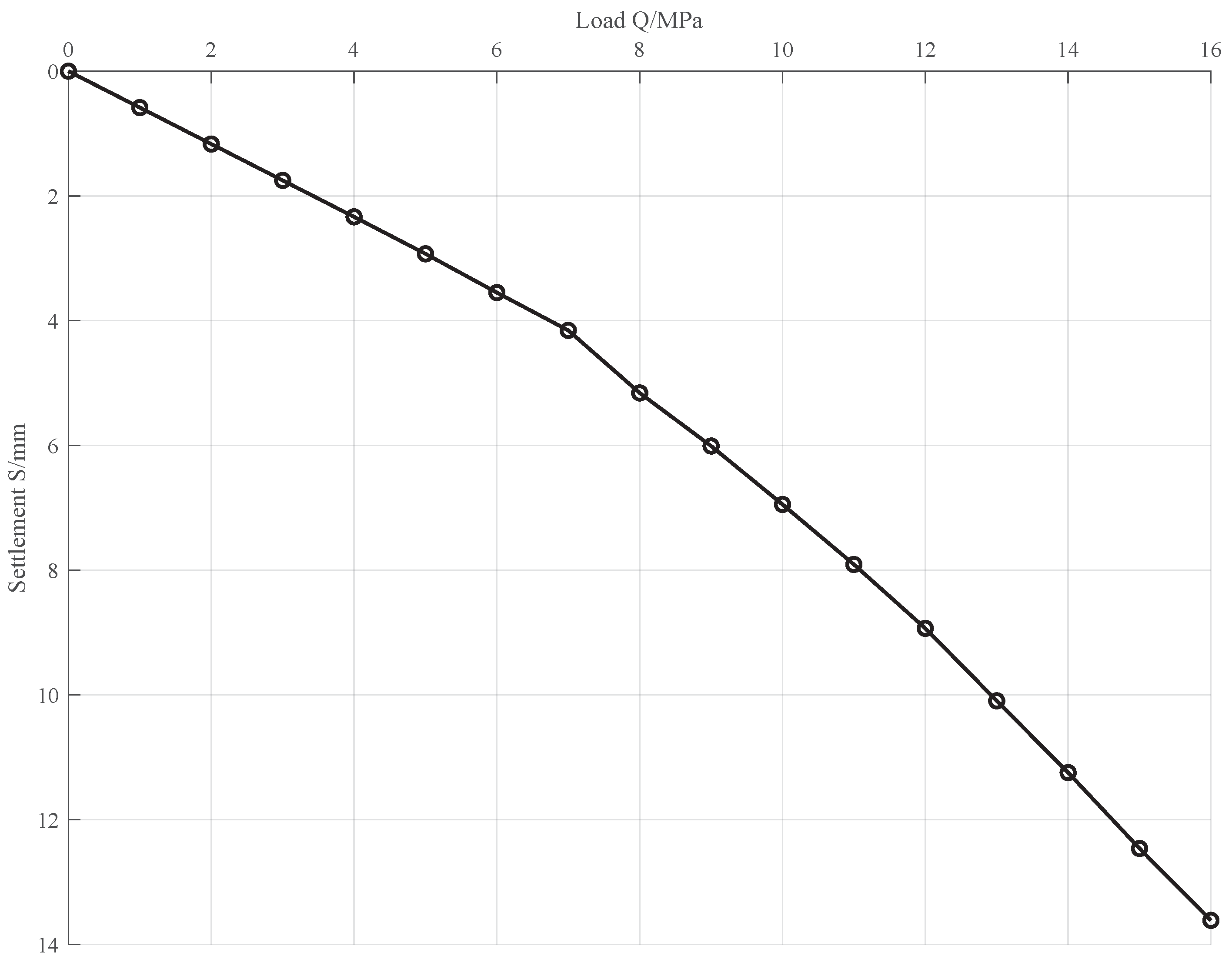
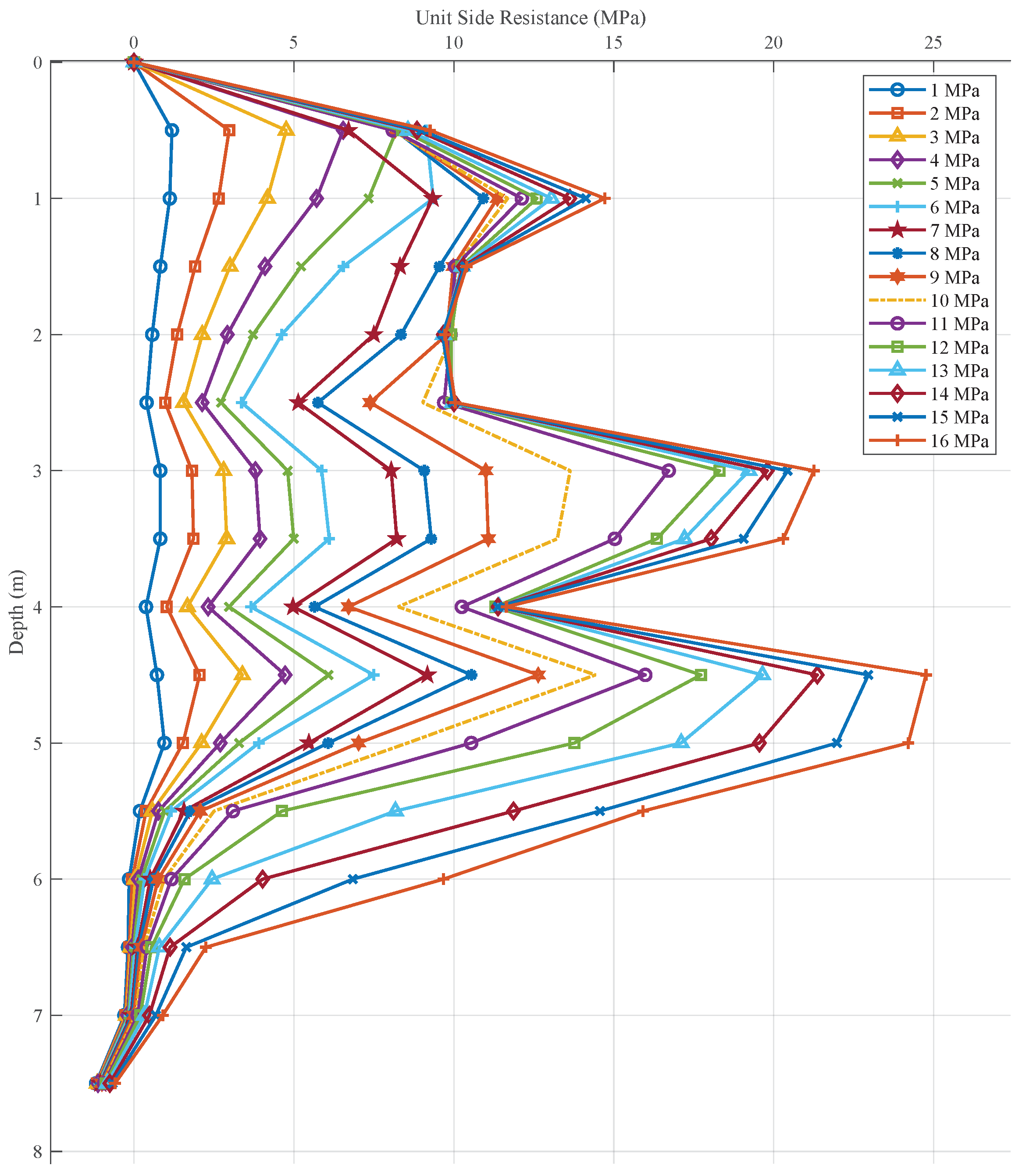
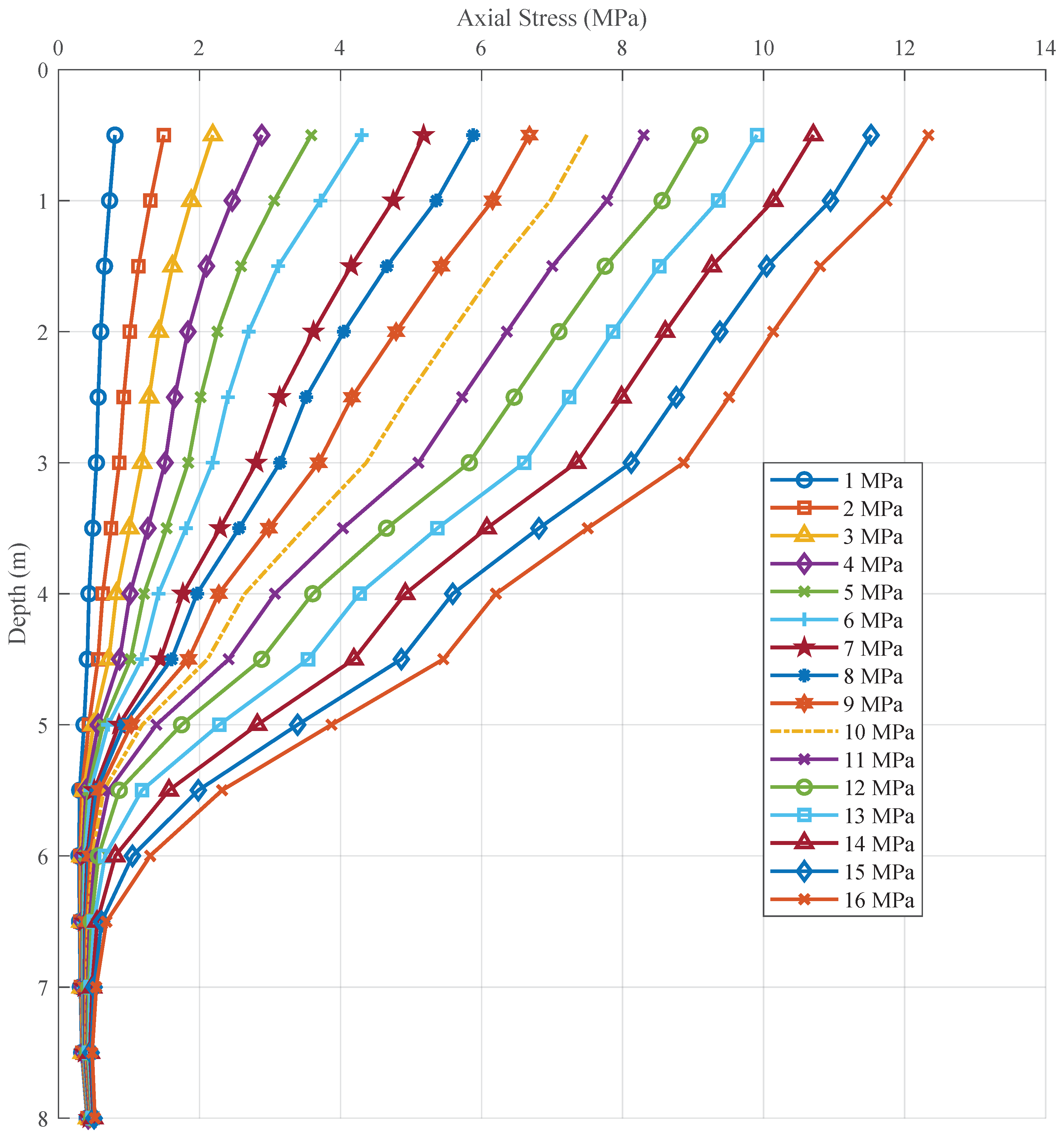
In Step 3, the load–displacement response of the pile foundation is resolved. First, the range and step size of the applied stress are determined. The stress is gradually applied to the top surface of the pile, and then increases again after equilibrium is reached. In this work, a step size of 1 MPa is employed until the specified maximum stress of 16 MPa is attained, which is achieved through the use of FISH loop construction. The large strain mode of FLAC is employed to guarantee the precision of the position and contact detection calculations and to forestall the model’s excessive movement in relation to one another, which could otherwise result in the failure of the solution. At the same time, the history of the stresses and displacements at the top and bottom of the pile are recorded, as are the stresses at different depths of the pile.

3. Experiments and Analysis

A rock-socketed pile created via rotary drilling was selected for examination in Gansu. The hole was not grouted due to the lack of water in the local environment, and the upper part was covered by an about 10 m layer of loess embedded in a rock layer at a depth of approximately 8.4 m, with a design hole diameter of 0.4 m. The borehole revealed the presence of three distinct rock strata, mudstone, sandstone and slate, from top to bottom. The borehole was scanned using the laser measurement system described above, which acquired approximately 2.5 million raw point cloud data points in three minutes.

3.1. Surface Modeling and Contour Line Roughness

The original point cloud was subjected to preprocessing and Delaunay triangulation, thereby creating a 3D surface model of the borehole. This reconstruction process was implemented on the basis of the PCL library. The reconstruction is shown in Figure 6. To obtain the contour lines of the drill holes, and calculate the roughness, the model is vertically sliced using a plane rotated along the center axis (z-axis). The angle of rotation of the plane ranges from 0 to 180°. The number of extracted contour lines is dependent upon the selected rotation step. In this study, the chosen rotation step is 45°, which results in 4 profiles and 8 contour lines. The extracted contour lines were coordinate transformed according to Equation (3) to form height undulations in the radius direction, as shown in Figure 7.

These contour lines were sampled at 1 mm intervals to calculate the $RF$ factor of the hole in different orientations, and the data are presented in

Table 1. $RF$ of contour lines in different directions.

Azimuth	0°	45°	90°	135°	180°	225°	270°	315°
RF	0.0231	0.0348	0.0612	0.0411	0.0432	0.0452	0.0213	0.0184

. As shown in Table 1, the hole is rougher in the 90° orientation, with an average value of 0.0360.

3.2. Load Simulation Results and Analysis

The pile–rock model is first subjected to preprocessing. The reconstructed surface model is imported into Rhinoceros 8 software for model processing, and rock models are established according to the actual situation. The subsurface 0∼3.5 m is mudstone, 3.5∼4.5 m is sandstone, and 3.5∼8.5 m is granite. The pile–rock model is subsequently merged into a nonmanifold mesh, which is then divided into volume entities to construct a 3D model comprising a volume mesh. The volume mesh is subsequently imported into FLAC3D for simulation purposes, as shown in Figure 8.

As detailed in Section 2.4, load simulations were conducted in FLAC3D.

Table 2. Material parameters for each model.

Parameters	Elastic Modulus ${\mathit{E}}_0$/Pa	Poisson’s Ratio $\mathit{\nu }$	Cohesion $\mathit{c}$/kPa	Friction Angle $\mathit{\phi }$/(°)	Density ρ/(kg/m3)
Pile	3.5 × 1010	0.30	-	-	2400
Mudstone	8 × 108	0.34	100	32	2080
Sandstone	2.1 × 109	0.29	150	37	2170
Slate	1.6 × 1010	0.25	200	42	2300

presents the model parameters for the concrete pile body and each rock layer used for the simulation. The material properties of the concrete were determined from the markers, and the rock material data were obtained from tests on field samples. The interface parameters were calculated using the recommended values in FLAC3D. The normal and shear stiffness of the interface was determined to be 2 × 10¹² Pa, while the friction angle and cohesion were established at 80 kPa and 25.6°, respectively. The density of the overlying loess layer was found to range from 1140 kg/m³ to 1890 kg/m³, with an intermediate value of 1500 kg/m³ taken for calculation purposes. Consequently, the surface applied ground stress was determined to be 150 kPa.

Figure 9 shows the load–displacement (Q–S) curve of the pile. The Q–S curve of this pile is generally slow-varying and relatively smooth without obvious inflection points, and the cutline stiffness $k_s$ ($k_s=Q/S$) decreases gradually with increasing displacement. The ultimate damage point of this rock-socketed pile is not obvious, the rate of change of settlement with an increasing loading in the experimental range still tends to be stable, and the surrounding rock offers greater side resistance. Therefore, when the pile parameters are designed, the ultimate bearing capacity is limited by an allowable settlement threshold.

Figure 10 shows the unit side resistance of the pile for different loads. The distribution of the pile side resistance does not exhibit a monotonic variation with depth but tends to increase and then decrease, reaching a peak at a depth of 4.5 m. This phenomenon is associated with both the displacement of strain and the type of rock mass. The displacement of the upper section is greater than that of the lower end, the shear expansion is relatively more pronounced, and the resulting stress is also greater. Moreover, the overall side resistance increases with an increasing load because as the pile moves downward due to the applied load, the sliding of the concave and convex surfaces along the interface induces radial expansion, which results in normal and shear stresses [26]. However, when the load exceeds a certain critical value (8 MPa), the side resistance in the middle and upper sections gradually stabilizes, whereas the side resistance in the lower section continues to increase. This indicates that at this point, the upper section has been destroyed by excessive displacement, and slip has occurred, whereas the lower section has not yet reached its ultimate side resistance and can continue to increase with increasing load.

Figure 11 shows the side resistance of different pile sections at relative pile-rock displacements. It is evident from the figure that the curve of the 0∼1 m pile section of the pile exhibits an inflection point, indicating that a greater side resistance is exerted at smaller displacements at this location. In contrast, the side resistance in the 4∼5 m pile section increases in a continuous manner, and the curve does not show any discernible inflection point. This is attributable to the presence of reaming at this location, which exhibits the most pronounced roughness, resulting in a larger ultimate side resistance. The overall curve of the pile demonstrates increased hardening, especially in the lower half of the pile.

Figure 12 shows the variation in the pile stresses under different loads. The figure shows that the pile axial force increases with increasing load, followed by a gradual decline in the depth direction. At each load, the pile shaft resistance and pile base resistance are present and less than the load, indicating that the shaft and base together carry their loads. The pile is an end-bearing friction pile. Moreover, the base carries a minimal percentage of the applied load, with the side resistance bearing the primary load. The degree of inclination of the pile shaft force along the depth direction is indicative of the degree of lateral resistance exerted on the pile. It was observed that as the magnitude of the applied load increased, the effect of side friction resistance also increased. Figure 13 shows the stress distribution of the pile–rock model under a load of 7 MPa. As shown in the figure, the stress distribution exhibits a similar phenomenon, with significantly higher stresses at the upper end of the region near the pile body, where most of the load is distributed. The pile stress decreases with depth, and the applied stress is gradually counteracted by the pile side resistance and transferred to the surrounding rock.

3.3. Analysis of Limit Side Resistance

Horvath fitted a relationship between the $RF$ roughness factor and the ultimate unit shaft resistance on the basis of the results of load tests on numerous bridge piers, as in Equation (4). Furthermore, the admissible value of the shaft resistance is presented and calculated via Equation (5), which should be considered in the design of piles.

$$q_{\mathrm{sL}}=0.8q_u{\left(\mathrm{RF}\right)}^{0.45}$$

(4)

$$q_s={\displaystyle \frac{\left(1-Q_b/Q_t\right)Q_t}{2\pi r_s{L}_s}}$$

(5)

where $q_u$ is the unconfined compressive strength, $Q_b$ is the bottom resistance, and $Q_t$ is the pile top load. $r_s$ and $L_s$ are the radius and length of the pile, respectively.

The roughness of the pile surface is not uniform, resulting in a constant variation in the unit shaft resistance along the depth direction. The results of the $RF$ calculations using contour lines in different directions were found to be variable. Therefore, the ultimate unit side resistance of the pile was calculated using the average $RF$ of the pile as 5.8 MPa, where $q_u$ is a typical value for concrete piles. In accordance with Figure 10, at the moment, the pile reached its upper limit, the applied load was 4 MPa and the depth was 0.5 m.

4. Conclusions

This paper presents a device for in situ measurement of socket sidewall roughness, and a numerical modeling method based on real measurement data. A laser scanning system for measuring the morphology of dry boreholes is designed to rapidly acquire numerous point clouds of the hole walls. The paper then outlines the process of extracting the roughness of the borehole from the surface model reconstructed from the point cloud, and proposes a method for load simulation in FLAC3D using the reconstructed 3D surface model. Compared with existing methodologies, the proposed approach offers a more realistic and comprehensive evaluation of the bearing performance of rock-socketed piles, providing a basis for decision-making in the construction design of rock-socketed piles. Under the condition of accurate parameter assignment, the side resistance and bearing capacity of the pile foundation can be predicted with greater accuracy.

A real borehole for a rock-socketed pile was tested and simulated, and the results demonstrated that the laser system accomplished the measurement of the borehole wall, and that the 3D model of the borehole was successfully constructed. On the basis of the reconstructed model, the roughness of the contour lines in different orientations was extracted, and the average $RF$ of the hole was 0.036. A load test was subsequently conducted in FLAC3D using the measured 3D model. The simulation results demonstrate that in this pile, the load is affected by both the side resistance and the end resistance, with the side resistance being the dominant factor. The ultimate bearing capacity can be selected by the settlement threshold.