Simulation Study of Deep Belief Network-Based Rice Transplanter Navigation Deviation Pattern Identification and Adaptive Control

Abstract

The navigation field of agricultural machinery has entered the intelligent stage, but the navigation control performance of paddy field agricultural machinery represented by rice transplanters is not stable in complex environments. Therefore, this study proposes a method to identify navigation deviation patterns based on Deep Belief Network (DBN) and designs an adaptive preview distance control method based on a driver preview model for each deviation pattern. Among them, the deviation pattern identification method is a two-stage algorithm. First, determine whether the current navigation status is abnormal. Then, the classification was refined for different abnormal states. The adaptive control method is divided into two levels. The main regulator calculates the dynamic preview distance according to the current state variable; the sub-regulator calculates the preview distance adjustment value according to the abnormal state degree. In the performance test of the identification method, all the models show excellent stability and accuracy, and the identification speed of the algorithm meets the high frequency of the rice transplanter navigation system. In the performance test of the control algorithm, compared with the static preview distance, the adaptive preview distance control method proposed in this study can effectively suppress the disturbance deviation of the rice transplanter navigation.

1. Introduction

Agricultural machinery navigation technology has been widely used in the field of intelligent agriculture [1,2]. Compared with dry fields, the stability and precision of rice transplanter navigation control in paddy fields are poor [3]. The ground structure of paddy fields is more complex, such as the mixture of mud and water, which causes the steering resistance and the poor steering control precision of agricultural machinery. Inconsistencies in the hardness of the paddy clay substrate can lead to bumpy bodywork and problems such as misalignment and sideslip.

In order to improve the stability and accuracy of navigation of agricultural machines, many researchers have focused on path-tracking control algorithms, and the preview model is the basis of traditional control algorithms. With a simple geometric algorithm for setting the preview point [4], the tracking control of different paths can be realized efficiently and flexibly. Compared with the classical control algorithms, Pure Pursuit has better tracking control performance at low speeds through simulation and comparative analysis [5]. The preview distance regulation strategy using PID [6] can minimize the preview error, which is characterized by a simple structure and a wide range of applications, but under transient conditions, the fixed PID weighting coefficients will cause the system to fail to respond in time, leading to an increase in the error.

These methods are only applicable to navigation control under steady-state conditions. Currently, control methods based on optimal control theory, such as linear quadratic regulator (LQR) [7] and model predictive control (MPC) [8], are widely used in various path-tracking scenarios. The cost function of the optimal control is composed of the errors of the variables within the preview model and has excellent performance for error prediction in dynamic environments. However, in nonlinear scenarios and complex environments, it can be computationally time-consuming or even without usable solutions [9].

Adaptive control methods incorporating deep learning are current research breakthroughs. In the application of system modeling, the method of the hybrid model can be used to correct the modeling error and obtain a high-accuracy system model [10]. In multi-degree-of-freedom complex systems, the use of radial basis neural networks (RBNNs) to adjust the state variables can effectively improve the stability of the system [11]. Many studies have shown that control methods incorporating deep learning can effectively improve the robustness, accuracy, and adaptive capability of control systems.

Deep learning methods are widely used in various fields due to their feature learning and identification capabilities. In the field of farmland environment sensing, farmland boundary information can be accurately and efficiently recognized using the Attention Gate (AG) mechanism and MultiResUnet [12]. However, it is difficult to improve the inference speed of the model due to the complex model structure and high computation. In the medical field [13] and environmental monitoring field [14], Deep Belief Network (DBN) has demonstrated strong generalization and efficient training capabilities.

In practical production studies, the main manifestation pattern of rice transplanter navigation instability is oscillation, which is motivated by sideslip [15,16,17] and systematic multi-error coupling. Therefore, realizing deviation pattern identification and adaptive regulation is an important way to improve the stability of rice transplanter navigation. For this reason, this study utilizes a deep learning approach to design an adaptive control method for suppressing deviation patterns. The main elements of this study include:

(1)

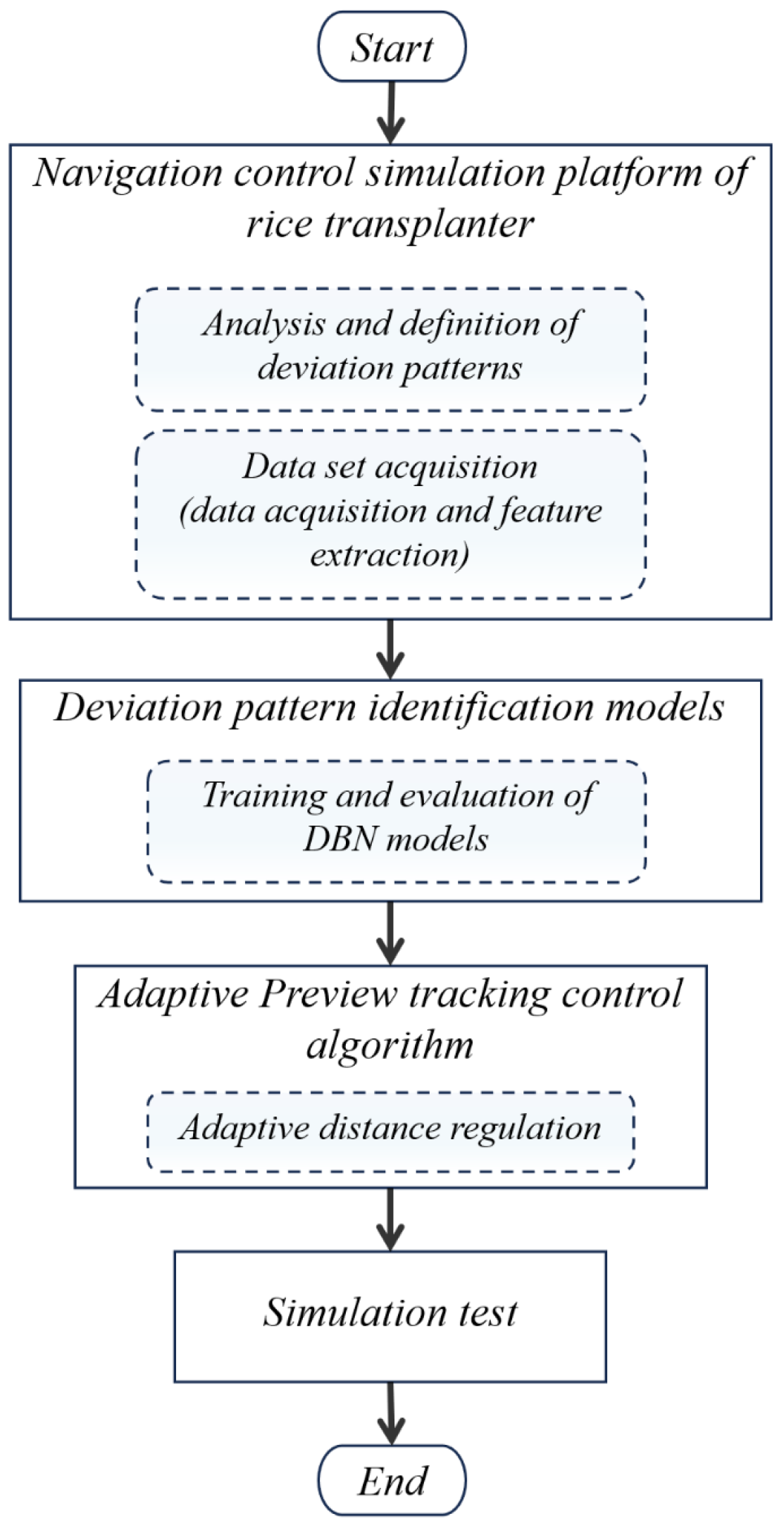
A rice transplanter navigation control simulation platform is designed. Simulating the state interference error during rice transplanter navigation operations provides a reliable and real experimental platform for subsequent research.

(2)

A deviation pattern identification method was designed. Based on the Deep Belief Network (DBN), three models were trained and implemented in two phases for real-time identification of deviation patterns.

(3)

An adaptive control method is designed. Based on the preview model, the optimal preview distance is adjusted in real time and the deviation is suppressed effectively.

2. Materials and Methods

In this study, a navigation control simulation platform of a rice transplanter was constructed in MATLAB/Simulink, and the navigation deviation pattern identification models and adaptive preview distance control algorithm were added to the platform. First, in the preliminary test, according to the defined deviation pattern, the key feature variables of navigation are analyzed and obtained, and the data set is made. Then, the deviation pattern identification models are designed and trained based on DBN. Finally, an adaptive preview distance control method is designed. The overall flow is shown in Figure 1.

2.1. Simulation Platform of Rice Transplanter Navigation Control

The simulation platform constructed in this study and all experiments were constructed in Windows 11, with Intel^® Core™ i7-10700 CPU, 16.0 GB RAM, and NVIDIA GeForce GT 730 GPU (Santa Clara, CA, USA). The software used was MATLAB/Simulink 2021a, and the simulation sampling time was 0.05 s (sampling frequency 20 Hz).

2ZGQ-80D Yangma rice transplanter (Syndmon International Co., Ltd., Changzhou, China) was taken as the research object (vehicle parameter setting), and the simulation platform is built by combining the functional units of the navigation control system, which mainly includes the sideslip kinematic model of the rice transplanter, the preview tracking control algorithm, the system measurement error generation module, and the path setting module. The overall structure is shown in Figure 2.

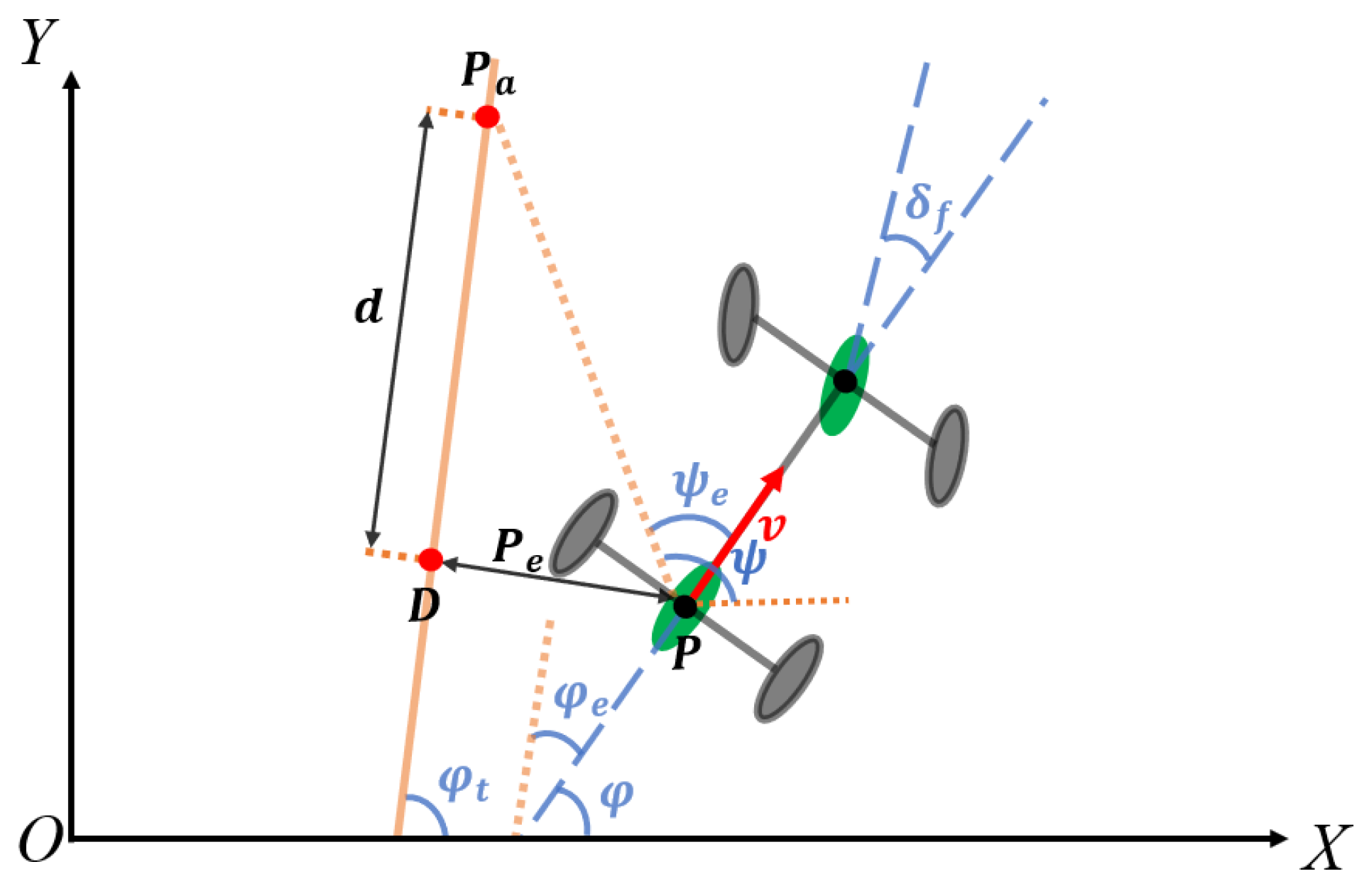
2.1.1. Sideslip Kinematic Modelling of Rice Transplanter

Due to the high complexity of the operation scene of the rice transplanter, when the narrow wheel is in contact with the mud surface, the dynamic parameters change dramatically, and it is difficult to estimate, and then the accuracy of the dynamic model cannot be guaranteed. Therefore, the simplified kinematic model of the rice transplanter is used instead of the dynamic model in this study.

The forward speed of the rice transplanter is slow, and it is regarded as a rigid body. Then, the kinematic model of the rice transplanter was constructed based on the Ackermann steering geometry principle. In order to simulate the sideslip state of a rice transplanter when traveling on a muddy and slippery road, the lateral speed $v_y$ is added to control point $P$, and the sideslip kinematics model is shown in Figure 3.

The parameters of the model are described in

Table 1. Parameterization of the kinematic model.

Symbol	Description	Symbol	Description
$\left(x,y\right)$	Position of control point $P$	$\phi$	Vehicle heading angle
$v$	Forward velocity	${\delta }_f$	Steering angle
${\nu }_y$	Lateral velocity	$l$	Wheelbase length
$\beta$	Sideslip angle	$R$	Turning radius

.

When the lateral speed $v_y=0$, the kinematic model of the rice transplanter is shown in Equation (1):

$$\left[\begin{array}{c}\dot{x}\\ \dot{y}\\ \dot{\phi }\end{array}\right]=\left[\begin{array}{c}cos\phi \\ sin\phi \\ {\displaystyle \frac{\tan {\delta }_f}{l}}\end{array}\right]v,$$

(1)

When there exists a lateral speed $v_y$ perpendicular to the vehicle, the sideslip angle $\beta$ and speed $V$ of the rice transplanter are shown in Equations (2) and (3).

$$\beta =arctan{\displaystyle \frac{v_y}{v}},$$

(2)

$$V={\displaystyle \frac{v}{cos\beta }}.$$

(3)

The simulation module is built in Simulink based on the sideslip kinematics model, and the status is updated after each sampling period.

2.1.2. Design of Preview Tracking Algorithm Based on Small Angle Linearization

In this study, a preview tracking control algorithm is designed based on the preview control theory [18], and its structure is shown in Figure 4.

The parameters and descriptions of the preview tracking model are shown in

Table 2. Parameterization of the preview model.

Symbol	Description	Symbol	Description
${\phi }_t$	Target heading angle	$d$	Preview distance
$P_a$	preview point	$P_e$	Position deviation
$\psi$	Preview heading angle	${\phi }_e$	Deviation to target heading angle
${\psi }_e$	Deviation to preview heading angle

.

Taking the preview straight line ${PP}_a$ as an auxiliary line, based on the small angle linearization method and the pole assignment method [19], the steering angle is obtained as

$${\delta }_f={\displaystyle \frac{2\cdot l}{\nu }}({\psi }_e+{\displaystyle \frac{1}{2\cdot \nu }}{p}_e),$$

(4)

where $p_e$ is the lateral deviation from control point $P$ to ${PP}_a$.

It can be seen as a rice transplanter always traveling along ${PP}_a$, when $p_e=0$ ($P$ is always on the ${PP}_a$), then Equation (4) is changed as

$${\delta }_f={\displaystyle \frac{2\cdot l}{\nu }}\left({\psi }_e+{\displaystyle \frac{1}{2\cdot \nu }}\cdot 0\right)={\displaystyle \frac{2\cdot l}{\nu }}{\psi }_e,$$

(5)

According to the preview tracking model, as shown in Figure 4,

$$\psi ={\phi }_t-arctan\left({\displaystyle \frac{P_e}{d}}\right),$$

(6)

$${\psi }_e=\phi -\psi ,$$

(7)

Therefore,

$${\psi }_e=\phi -\psi +arctan\left({\displaystyle \frac{P_e}{d}}\right)={\phi }_e+arctan\left({\displaystyle \frac{P_e}{d}}\right).$$

(8)

The optimal steering angle can be obtained by Equations (5) and (8) as

$${\delta }_f=k\left({\phi }_e+arctan\left({\displaystyle \frac{P_e}{d}}\right)\right).$$

(9)

2.1.3. Systematic Measurement Error Generation Module

In the actual environment, there is a systematic measurement error in the state quantity of the navigation system. The rice transplanter navigation system generally selects a dual-antenna scheme, and the measurement error of its heading fluctuates very slightly in the dynamic environment, so the heading perturbation is not considered. In order to simulate the measurement error of the rice transplanter navigation system, this study adds positioning noise and steering noise to the simulation platform.

(1)

Positioning measurement error

Add measurement errors, $x_e$, $y_e$, at vehicle control point $P$: The rice transplanter navigation system utilizes RTK-GNSS technology to achieve high-precision positioning, and its measurement accuracy can reach below 0.02 m with a dynamic error range of 0.01~0.02 m [20,21]. Therefore, the positioning measurement error $x_e$, $y_e$ (mean 0 m, variance 0.0004 m², normal distribution) in the X-Y direction was added to the control point $P$ of the rice transplanter.

(2)

Steering control error

The control error ${\delta }_{fe}$ and lag time $\tau$ are added to the steering control: In the steering control of the rice transplanter, the control error will appear due to the high steering resistance and the untimely control response. The rice transplanter navigation system utilizes the steering wheel motor to achieve steering control, with an error standard deviation of 1° and an average steering lag time of 0.3 s [22,23,24]. In this study, the steering angle control error ${\delta }_{fe}$ (mean 0°, variance 1, normal distribution) and steering lag time $\tau$ (mean 0.3 s, variance 0.04, normal distribution) were added at the steering angle.

2.1.4. Navigation Path Setting Module

Path setting is an important part of the navigation process for agricultural machines. The workflow of the path-setting module designed in this study is described below:

(1)

Enter the measured position $P^{\prime }=(x+x_e,y+y_e,)$ of the rice transplanter control point $P$ and its heading angle $\phi$.

(2)

Set the target heading angle ${\phi }_t$, forward speed $v$, and extend the navigation line ${Line}_{AB}$ from the starting point.

(3)

Calculate the heading angle deviation ${\phi }_e$ between $\phi$ and ${\phi }_t$, and the position deviation $P_e$ between $P^{’}$ and ${Line}_{AB}$, and output ${\phi }_e$ and $P_e$.

Eventually, the information is input to the preview tracking control algorithm.

2.2. Definition and Analysis of Path-Tracking Deviation Pattern

In the navigation process of the rice transplanter, due to the external environment interference and untimely execution of control decisions, the path tracking state is caused to have an abnormal state, which is mainly manifested as oscillation and sideslip. In order to construct an effective dataset, this section defines the deviation pattern and its degree by analyzing the data curves of the navigation state and clarifies the key characteristic variables through theoretical analysis.

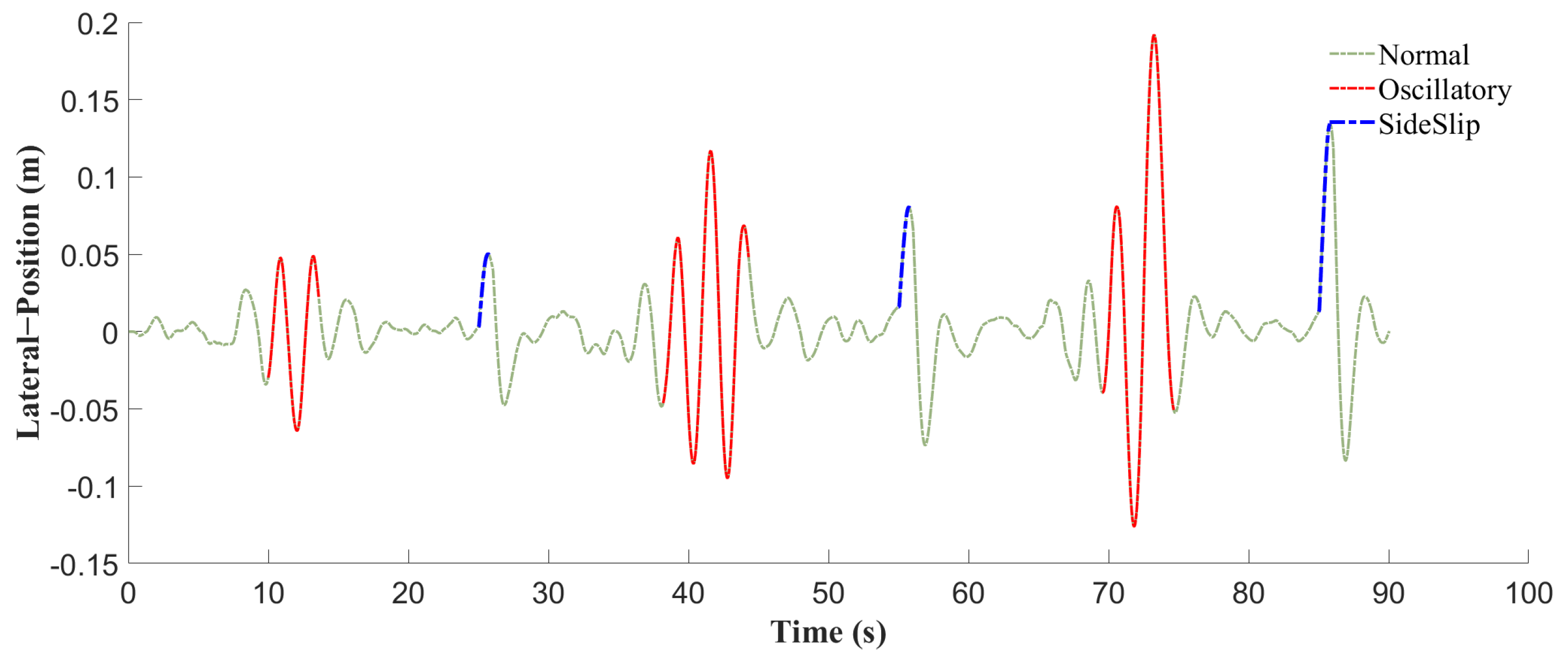
2.2.1. Definition of Path-Tracking Deviation Patterns

Based on the real data of navigation state quantities (without adding systematic measurement errors), each deviation pattern is divided according to the variation interval of the real data curve.

• Classification of abnormal states

In order to distinguish the rice transplanter path tracking deviation patterns, the navigation anomaly states are classified into three types, as shown in

Table 3. Rules for classifying the abnormal states.

Abnormal State	Classification Criteria	Label
Normal	$(P_{e\_max}<0.05 \mathrm{m}) \mathrm{a}\mathrm{n}\mathrm{d} ({\phi }_{e\_max}<3°)$	1
Oscillation	$(P_{e\_max}\ge 0.05 \mathrm{m}) \mathrm{o}\mathrm{r} ({\phi }_{e\_max}\ge 3°)$	2
Sideslip	$\beta \ge 4$	3

.

Where $P_{e\_max}$ is the maximum position deviation in the data curve, ${\phi }_{e\_max}$ is the maximum heading deviation in the data curve, and $\beta$ is the sideslip angle in the data curve.

2.

Classification of degree of oscillation

In order to distinguish the categories of oscillatory states in a more detailed way, the degree of oscillation was classified into three types, as shown in

Table 4. Rules for classifying the degree of oscillation.

Degree of Oscillation	Classification Criteria	Label
Mild	$0.05 m<P_{e\_max}\le 0.10 m$	1
Moderate	$0.10 m<P_{e\_max}\le 0.15m$	2
Severe	$0.15 m<P_{e\_max}$	3

.

3.

Classification of Degree of Sideslip

In order to distinguish the categories of sideslip status in a more detailed way, the degree of sideslip was classified into three types, as shown in

Table 5. Rules for classifying the degree of sideslip.

Degree of Sideslip	Classification Criteria	Label
Mild	$4°<\beta \le 6°$	1
Moderate	$6°<\beta \le 8°$	2
Severe	$8°<\beta$	3

.

2.2.2. Key Characteristic Variables of Path-Tracking Deviation Patterns

In order to construct a dataset with significant features, the key feature variables under each deviation pattern are clarified by analyzing the dynamic correlation characteristics of each functional module in the simulation platform.

• Key characterization variables in oscillation states

When the rice transplanter did not sideslip, the change rule of the state variables conformed to the kinematic model. At this time, the rate of change of position deviation is the longitudinal speed of the rice transplanter about the target path.

$$\dot{P_e}=v\cdot \sin {\phi }_e,$$

(10)

The rate of change in heading deviation is equal to the rate of change in heading.

$$\dot{{\phi }_e}=v\cdot {\displaystyle \frac{\tan {\delta }_f}{l}},$$

(11)

From Equations (10) and (11), combined with the classification rules of the path-tracking oscillation pattern, linear characteristics of $P_e$, ${\phi }_e$, and ${\delta }_f$ can be used to directly characterize whether oscillation occurs.

2.

Key characterization variables in sideslip states

The rice transplanter sideslip process can be regarded as a navigation path tracking process with small angle changes in heading when $P_e$ changes drastically and ${\phi }_e$ does not change significantly.

From Equation (9), it can be seen that when ${\phi }_e$ changes very little, ${\delta }_f$ is more sensitive about the response of $P_e$, and in the process of sideslip, the relationship between the three changes is nonlinear; at this time, it can be based on this nonlinear feature to determine whether sideslip occurs.

In summary, it can be clarified that the key characteristic variables of the deviation pattern of rice transplanter navigation path tracking are $P_e$, ${\phi }_e$, and ${\delta }_f$, respectively.

2.3. DBN-Based Path-Tracking Deviation Pattern Identification Model and Dataset Preparation

In the application of deep learning, related studies have shown that the structural properties of Deep Belief Networks (DBNs) are adapted to 1D or 2D feature learning [13,14], which can effectively recognize and classify each deviation pattern.

2.3.1. Training of DBN

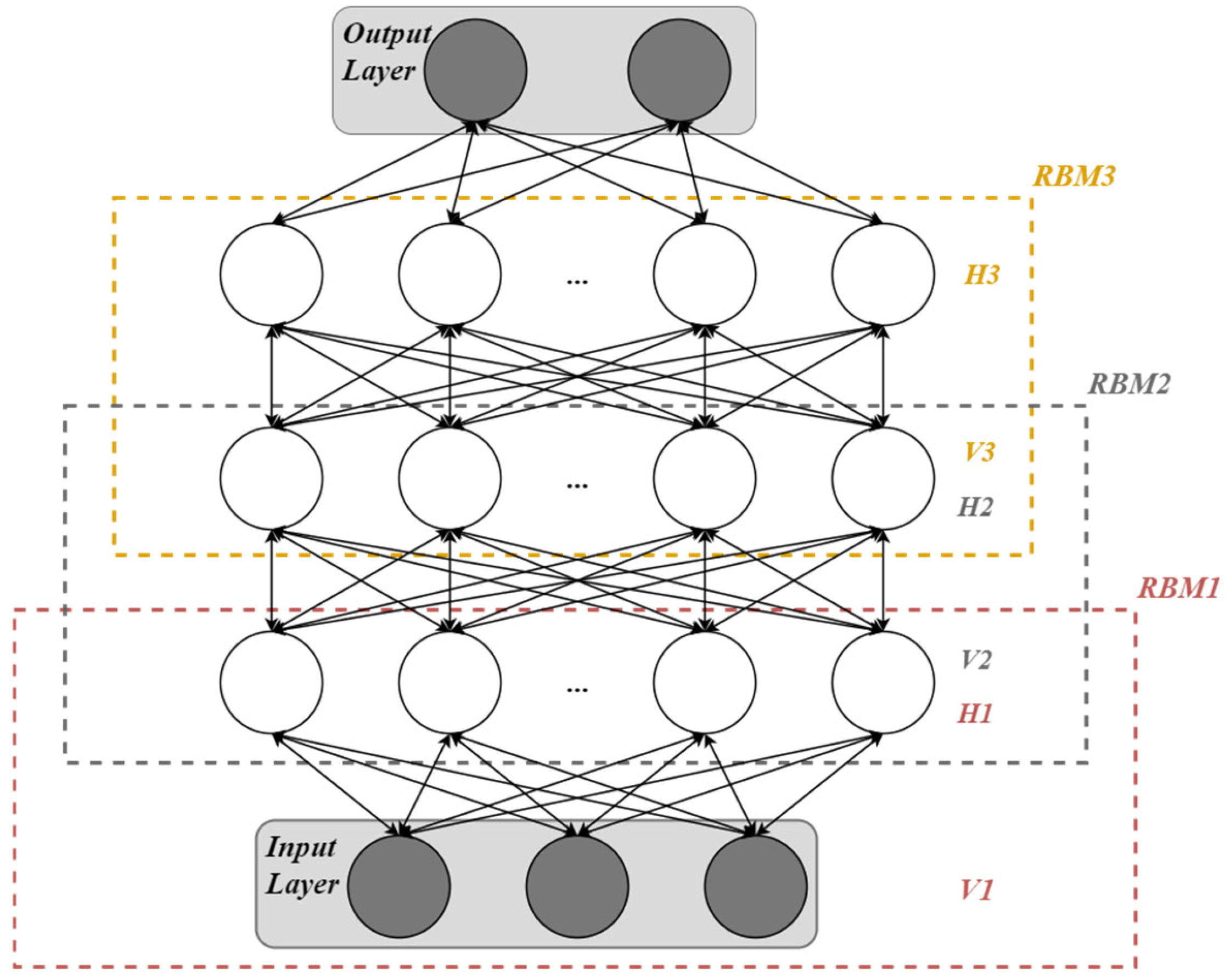
• Structure of DBN

Deep Belief Network (DBN) is essentially a probabilistic generative model, which is a multilayer perceptual network stacked with Restricted Boltzmann Machine (RBM) [25], which centers on a layer-by-layer greedy learning algorithm [26]. The DBN training is divided into two phases: first, an unsupervised pre-training phase, followed by a supervised backward fine-tuning phase (which can be viewed as a BP session). Its overall structure is shown in Figure 5.

The RBM is divided into visible and hidden layers; there are omnidirectional connections between the nodes in the visible and hidden layers, and the nodes within the layers are unconnected. Its internal structure is shown in Figure 6.

During training, nodes within the visible layer obtain features from the dataset and pass them to the hidden layer. Then, the nodes within the hidden layer multiply them with the weights to obtain the bias and add it to the result. The output is processed through the activation function and passed to the next hidden layer again. This hierarchical learning approach not only improves the learning efficiency of DBN; it also enhances the multi-feature extraction capability of the model.

2.

Unsupervised pre-training process

In the pre-training phase, the probability distribution function $p(V,H)$ is shown in (12).

$$p\left(V,H\right)={\displaystyle \frac{e^{-E(V,H)}}{N}}$$

(12)

where $E(V,H)$ is the energy function and $N$ is a normalization constant.

The energy function $E(V,H)$ of the visible and hidden layer nodes is

$$E\left(V,H\right)=-({\sum }_{i=1}^n{a}_i{·V}_i+{\sum }_{j=1}^m{b}_j·H_j+{\sum }_{i=1}^n{\sum }_{j=1}^m{W}_{ij}{·V}_i{·H}_j)$$

(13)

where $a_i$ is the deviation of the visible layer, $b_j$ is the deviation of the hidden layer, $V_i$ is the node of the visible layer, $H_j$ is the node of the hidden layer, and $W_{ij}$ is the connection weight between the visible and hidden layers.

The normalization constant $N$ is the sum of the energy of all nodes between the visible and hidden layers.

$$N={\sum }_V{\sum }_H{e}^{-E(V,H)},$$

(14)

In the process of unsupervised learning, the log-likelihood function is key to the model and reflects the model’s learning ability.

$$L={\sum }_{z=1}^l\mathit{ln}p\left(V,H\right),$$

(15)

where $l$ denotes the sum of all training data.

During the RBM training process, the Contrastive Divergence (CD) method is utilized to update the weights $W_{ij}$ and deviations $a_i$, $b_j$ of the visible and hidden layers. The CD algorithm is shown in Equations (16)–(18).

$$∆W_{ij}=\theta ·\left[{\left(V_i{·H}_j\right)}_{Label}-{\left(V_i{·H}_j\right)}_{Predict}\right],$$

(16)

$$∆a_i=\theta ·\left[{\left(V_i\right)}_{Label}-{\left(V_i\right)}_{Predict}\right],$$

(17)

$$∆b_j=\theta ·\left[{\left(H_j\right)}_{Label}-{\left(H_j\right)}_{Predict}\right],$$

(18)

where $\theta$ denotes the learning rate, ${\left(·\right)}_{Label}$ denotes the value of the actual data, and ${\left(·\right)}_{Predict}$ denotes the value of the predicted data.

3.

Supervised reverse fine-tuning process

After the pre-training process, the reverse fine-tuning begins. In this process, the model is updated cyclically based on the weights $W_{ij}$, the node bias $b_j$ of the hidden layer, and the loss function $E_{Loss}$. The formula is shown in Equations (19) and (20).

$$W_{ij}=W_{ij}-\theta ·{\displaystyle \frac{\partial E_{Loss}}{\partial W_{ij}}},$$

(19)

$$b_j=b_j-\theta ·{\displaystyle \frac{\partial E_{Loss}}{\partial b_j}} ,$$

(20)

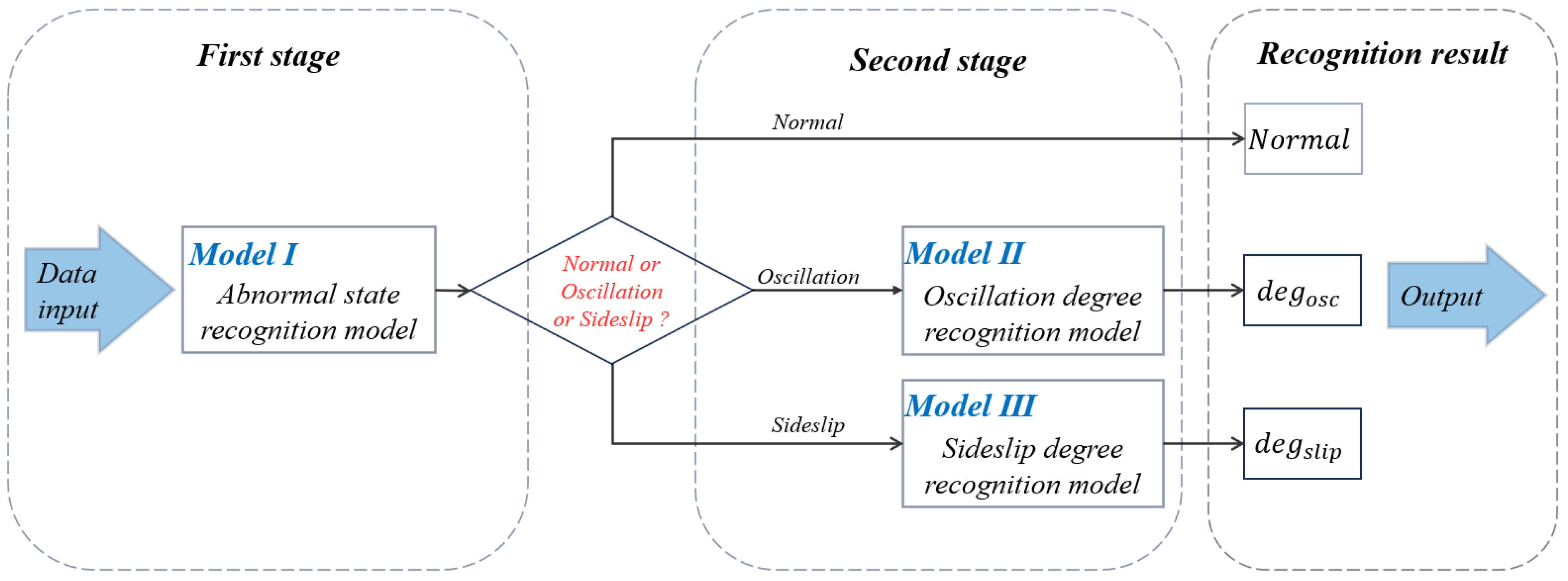
2.3.2. Design of the Deviation Pattern Identification Model

As analyzed by Section 2.2.2, the association characteristics of each deviation pattern with different state variables are inconsistent. In order to avoid the problem of poor learning effect of a single DBN model, this study trained three models for the application scenarios of multiple deviation patterns. The description of each model is shown in

Table 6. Functional description of each model.

Model	Input	Output	Description
I	State Variable Characterization Dataset	Normal or Oscillation or Sideslip	Identify abnormal states (The division rules are shown in Table 3)
II		Degree of Oscillation ${(deg}_{osc})$	Identify the degree of Oscillation (The division rules are shown in Table 4)
III		Degree of Sideslip ${(deg}_{slip})$	Identify the degree of sideslip (The division rules are shown in Table 5)

.

The workflow of each model: In the first stage, the data are input to Model I; if the identification result is normal, then there is no need to call the subsequent models; if the identification result is oscillation or sideslip, start the second stage; the data are input to Model II or Model III to identify the degree of oscillation or sideslip. The workflow is shown in Figure 7.

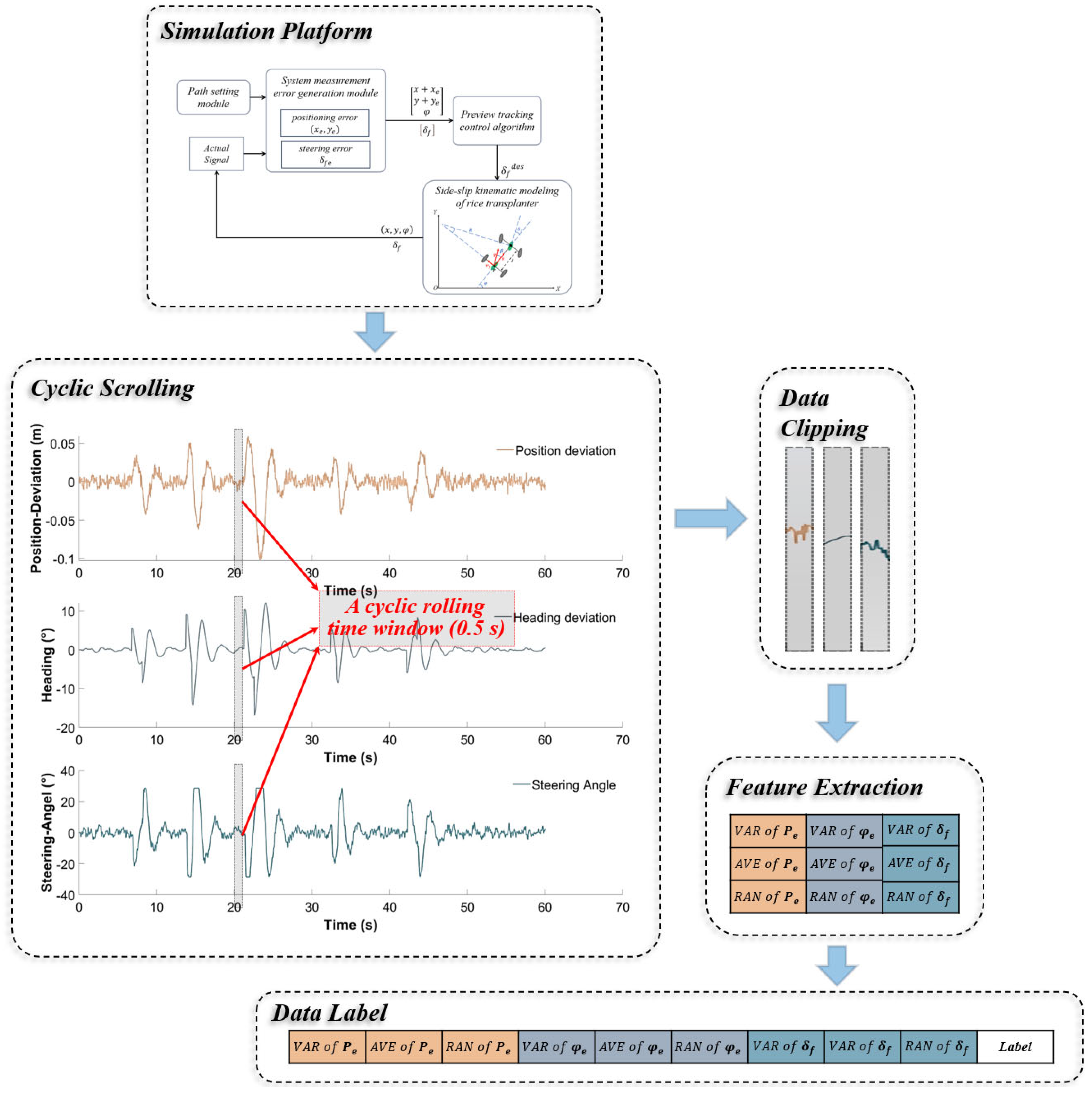
2.3.3. Data Acquisition and Feature Extraction

Based on the simulation platform shown in Figure 2, the raw data of path tracking under the systematic error conditions were obtained, and the data curve slices were intercepted in the 0.5 s time range. The features of the raw data curve slices are refuted, unclear and pointing. Further, the data features were simplified and generalized. Extracting the mean, variance, and extreme deviation of the raw data curve slices as a new dataset prevents the effects of system noise and data interference on the dataset.

The dataset production process is shown in Figure 8:

(1)

Traversing the raw data curves of the navigation key feature variables (position deviation $P_e$, heading deviation ${\phi }_e$, and steering angle ${\delta }_f$) using a circular scrolling time window (0.5 s in length);

(2)

According to the path-tracking deviation pattern defined in Section 2.2.1, the data curves under the corresponding time window are intercepted, split, reorganized, and labeled for classification in the form of arrays.

(3)

Extract the mean, variance, and extreme deviation of the raw data curve slices, save the data to the workspace in the MATLAB platform, and finally export and save it as a .xlsx file.

2.3.4. Dataset Segmentation

To ensure the reasonableness of the dataset, firstly, the dataset of each model is randomly divided into 10 parts, of which 9 are the training set and 1 is the testing set; then, the training set is further divided into 10 parts, of which a certain 1 part is rotated as the validation set, and the remaining 9 parts are used as the training set. Each model has three types of data set types, and each type has 1000 data samples, which totals 9000 data samples for the three models. The data set division for each model is shown in

Table 7. Scale of dataset partitioning for each model.

Dataset	Percentage	Actual Number
Training	90%·90%	2430
Validation	90%·10%	270
Testing	10%	300
Full Data	100%	3000

.

2.4. Design of Adaptive Preview Control Algorithm

Preview tracking control has been widely adopted because of its good path-tracking effect [10,18]. In order to cope with the complex paddy field environment, this study proposes an adaptive preview tracking control algorithm based on the preview model by combining the deviation pattern identification method. The algorithm consists of a main regulator and a sub-regulator:

(1)

The main regulator calculates the basic preview distance to ensure stable control of the system under undisturbed conditions;

(2)

The sub-regulator calculates the preview distance adjustment value to ensure that the system quickly suppresses deviation under disturbing conditions.

The two regulators work together to make the rice transplanter navigation system adaptively adjust the preview distance under steady-state and non-steady-state conditions. The overall workflow of the algorithm is shown in Figure 9.

2.4.1. Design of the Main Regulator

In order to ensure the timely convergence and stability of rice transplanter navigation without disturbance, the main regulator is designed based on the preview control method. Taking the forward speed $v$, position deviation $P_e$, and steering control lag time $\tau$ as factors, and the critical oscillation state as the judgment basis, the basic preview distance $d$ that ensures the system does not oscillate under the condition of no perturbation is matched under the condition of no perturbation with different factors.

When the rice transplanter navigates the operation in the paddy field, the traveling speed $v$ is 0.75~1.5 m/s, and the position deviation $P_e$ when stabilized on the line is in the range of 0~0.1 m, and its steering control lag time $\tau$ can be viewed as a number with a mean value of 0.3 s and a normal distribution. Therefore, the setup test parameters and results are shown in

Table 8. Matching test results for basic preview distance $d$.

Index	$\mathit{v}$ (m/s)	${\mathit{P}}_{\mathit{e}}$ (m)	$\mathit{\tau }$ (s)	$\mathit{d}$ (m)
1	0.90	0.04	0.18	0.25
2	1.35	0.04	0.18	0.35
3	0.90	0.08	0.18	0.40
4	1.35	0.08	0.18	0.45
5	0.90	0.04	0.42	0.65
6	1.35	0.04	0.42	0.90
7	0.90	0.08	0.42	0.75
8	1.35	0.08	0.42	1.00
9	0.75	0.06	0.30	0.45
10	1.50	0.06	0.30	0.65
11	1.13	0.02	0.30	0.45
12	1.13	0.10	0.30	0.65
13	1.13	0.06	0.10	0.30
14	1.13	0.06	0.50	1.05
15	1.13	0.06	0.30	0.55

.

The output of the main regulator is set to be the basic preview distance $f_{main}$, whose value is equal to $d$. With $v$, $P_e$, and $\tau$ as the independent variables and $d$ as the dependent variable, the expression Equation (21) for the main regulator was fitted using the least squares method based on the data in Table 8.

$$\begin{gathered} f_{main}=d=0.180826-0.096112·v+4.42955·P_e-1.67884·\tau \\ -1.17851·v·P_e+1.64992·v·\tau -2.20971·P_e·\tau \\ -0.001885·v^2-0.165695·{P_e}^2+3.11837·{\tau }^2\hspace{1em}. \end{gathered}$$

(21)

2.4.2. Design of the Sub-Regulator

• Definition of sub-regulator

The sub-regulator, as a supplement to the main regulator, and when the system oscillates or sideslips under perturbation conditions, the preview distance is adjusted adaptively according to the results of the deviation pattern identification, and the deviation is suppressed quickly.

The output of the sub-regulator is set to be the preview distance adjustment value $f_{sub}$, whose expression equation is shown in Equation (22).

$$f_{sub}=f_{sub\_osc}+f_{sub\_slip},$$

(22)

where $f_{sub\_osc}$, $f_{sub\_slip}$ are the preview distance adjustment values for oscillation and sideslip (as a function of ${deg}_{osc}$ and ${deg}_{slip}$).

Define the oscillation adjustment coefficient $A$ and the sideslip adjustment coefficient $B$, and rewrite Equation (23) as

$$f_{sub}=A·{deg}_{osc}+B·{deg}_{slip},$$

(23)

According to the rules and labels in Table 4 and Table 5, ${deg}_{osc}\in \left(\mathrm{1,2},3\right)$ and ${deg}_{slip}\in \left(1,2,3\right)$ in Equation (23).

2.

Setting constraints

The length of the preview distance is related to the speed. The traveling speed $v$ of a rice transplanter is generally in the range of 0.75~1.5 m/s. In order to ensure the system has a good control response, the preview distance should not be too large or too small. Therefore, on the basis of the main regulator, limit $f_{sub}$, constituting the constraints as shown in Equation (24).

$$0 < A·{deg}_{osc}+B·{deg}_{slip} < 2·v,$$

(24)

From the above analysis, $A$ and $B$ should be taken in the range of 0 to 1.

3.

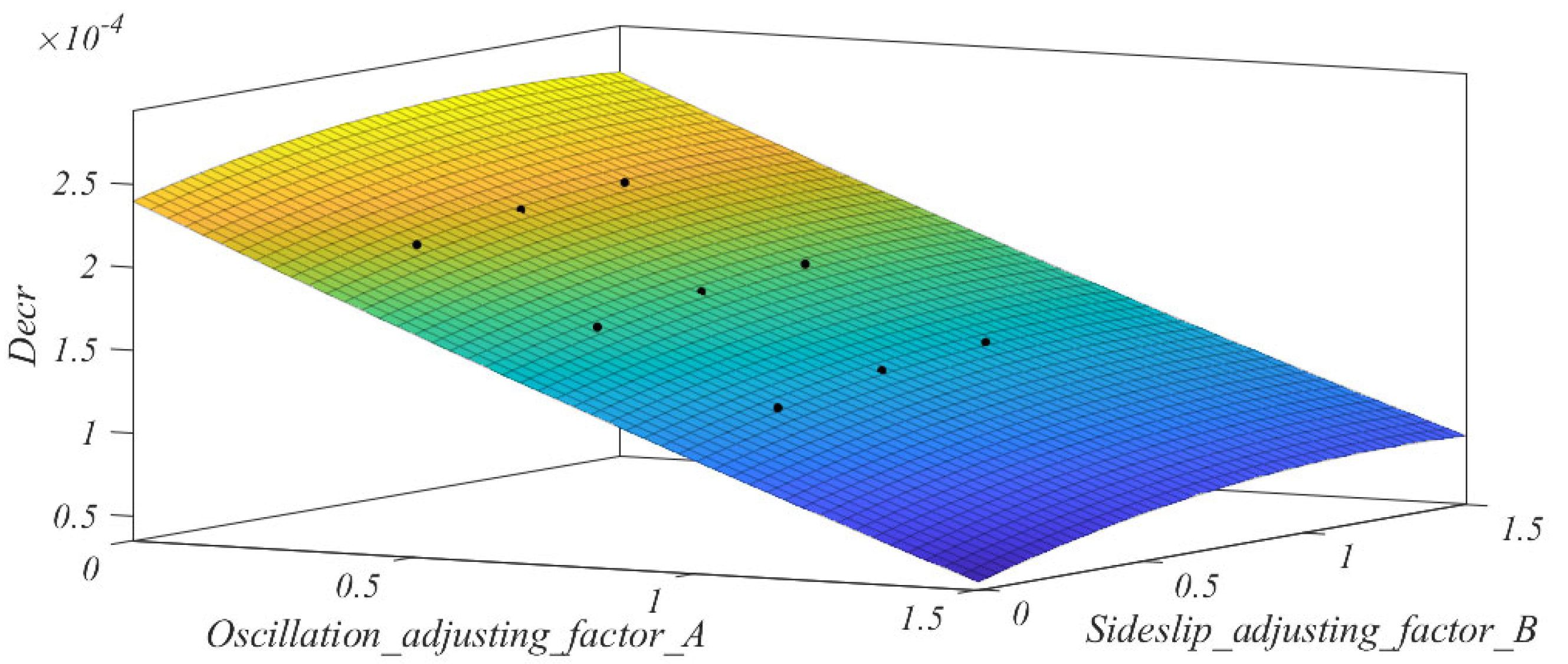
Optimal adjustment factor test

Further, in order to select the optimal adjustment coefficients A and B, a control test was carried out on the rice transplanter navigation control simulation platform:

(1)

At a $v=0.8 \mathrm{m}/\mathrm{s}$, the control curve is set up as shown in Figure 10. Specifically, on the basis of the main regulator (the sub-regulator does not intervene), three degrees of oscillations are induced by narrowing the preview distance, and three degrees of sideslip are induced by applying different degrees of lateral velocity. The overall variance of the control curves ${VAR}_{refer}=0.0022 \mathrm{m}$.

(2)

Set $A$ and $B$ as multiple groups of level factors (value range 0~1), intervene the sub-regulator on the basis of the main regulator, i.e., add the preview distance adjustment value as shown in Equation (23), carry out the simulation test with different adjustment coefficients, and obtain the overall variance ${VAR}_{test}$ of each tracking curve.

(3)

The declining variance ${Devr}_{test}$ of each tracking curve is used as an evaluation index, as shown in Equation (25).

$${Decr}_{test}={VAR}_{refer}-{VAR}_{test},$$

(25)

The test results are shown in

Table 9. Coefficient comparison test results.

Index	Coefficient		${\mathit{V}\mathit{A}\mathit{R}}_{\mathit{t}\mathit{e}\mathit{s}\mathit{t}}$/m2	${\mathit{D}\mathit{e}\mathit{c}\mathit{r}}_{\mathit{t}\mathit{e}\mathit{s}\mathit{t}}$/m2
	$\mathit{A}$	$\mathit{B}$
1	0.96	0.96	0.001125	0.000140
2	0.96	0.64	0.001131	0.000134
3	0.96	0.32	0.001143	0.000123
4	0.64	0.96	0.001084	0.000181
5	0.64	0.64	0.001090	0.000175
6	0.64	0.32	0.001100	0.000165
7	0.32	0.96	0.001041	0.000224
8	0.32	0.64	0.001047	0.000218
9	0.32	0.32	0.001057	0.000208

.

With $A$ and $B$ as the independent variables and ${Decr}_{test}$ as the dependent variable, the expression in Equation (26) was fitted using the least squares method.

$${Decr}_{test}=\left(2.37-1.35·A+0.519·B+0.046·A·B-0.228·B^2\right)·{10}^{-4},$$

(26)

The response surface of Equation (26) is plotted, as shown in Figure 11.

From the response surface analysis, it can be seen that the ${Devr}_{test}$ decreases with the increase in the $A$ and increases first and then decreases with the increase in the $B$. In the range of the constraint interval, the values of $A$ and $B$ at the highest point of the selected surface are (0.288, 0.992), i.e., the optimal regulation coefficients, when the theoretical variance decrease value ${Devr}_{test}$ of the tracking control curve is the largest.

3. Results and Analysis

3.1. Path-Tracking Deviation Pattern Identification Test

3.1.1. Test Preparation

• Evaluation Index

In this study, the performance of the DBN model was carried out using the K-Fold cross-validation method, and the performance of each model was assessed by calculating Loss, MAE, Macro-F1 and Accuracy as in Equations (27)–(30).

$$\mathrm{L}\mathrm{o}ss:-{\displaystyle \frac{1}{M}}{\sum }_{j=1}^M{\sum }_{i=1}^N{y}_{ij}\log \left({\widehat{y}}_{ij}\right),$$

(27)

$$\mathrm{M}\mathrm{A}\mathrm{E}:{\displaystyle \frac{1}{M}}{\sum }_{i=1}^M{|y}_i-{\widehat{y}}_i|,$$

(28)

$$Macro-F1:mean\left({\displaystyle \frac{2·TP}{2·TP+FP+FN}}\right),$$

(29)

$$Accuracy\left(\%\right):{\displaystyle \frac{TP+\mathrm{T}\mathrm{N}}{\mathrm{T}\mathrm{P}+\mathrm{F}\mathrm{P}+\mathrm{F}\mathrm{N}+\mathrm{T}\mathrm{N}}}\times 100,$$

(30)

where $M$ is the number of samples, $N$ is the number of categories, $y$ is the sample label, and $\widehat{y}$ is the prediction label.

2.

Parameters of DBN

DBN performance is affected by a variety of hyperparameters, including the number of hidden layers, the number of hidden layer nodes, and the learning rate. Referring to DBN parameter setting [27], a DBN with a structure of 9-100-100-3 is set up based on engineering experience (trial-and-error method), and the parameters are shown in

Table 10. Parameters and description of DBN model.

Parameters	Value	Description
$L_{input}$	9	Number of nodes in the input layer, corresponds to the number of features
$L_{s1}$	100	Number of nodes in the hidden layer 1
$L_{s2}$	100	Number of nodes in the hidden layer 2
$B_{pre}$	10	Batch size of pre-training
$L{R}_{pre}$	$0.35$	Learning rate of pre-training
$E_{pre}$	100	Epoch of pre-training
${LS}_{pre}$	0.999	Learning rate scale factor of pre-training
$B_{ret}$	10	Batch size of reverse fine-tuning
$L{R}_{ret}$	0.50	Learning rate of reverse fine-tuning
$E_{ret}$	50	Epoch of reverse fine-tuning
${LS}_{ret}$	0.999	Learning rate scale factor of reverse fine-tuning
$L_{output}$	3	Number of nodes in the output layer corresponds to the number of categories

.

Where the learning rate scale factor $LS$ is multiplied by the learning rate $LR$ to update the learning rate and prevent the model from overfitting due to too large a learning rate. The number of nodes in the input layer $L_{input}$ is equal to the number of features in the dataset, and the number of nodes in the output layer $L_{output}$ is equal to the total number of categories in the data labels. Other model hyperparameters, such as the number of nodes, batch size, learning rate, etc., need to be adjusted empirically.

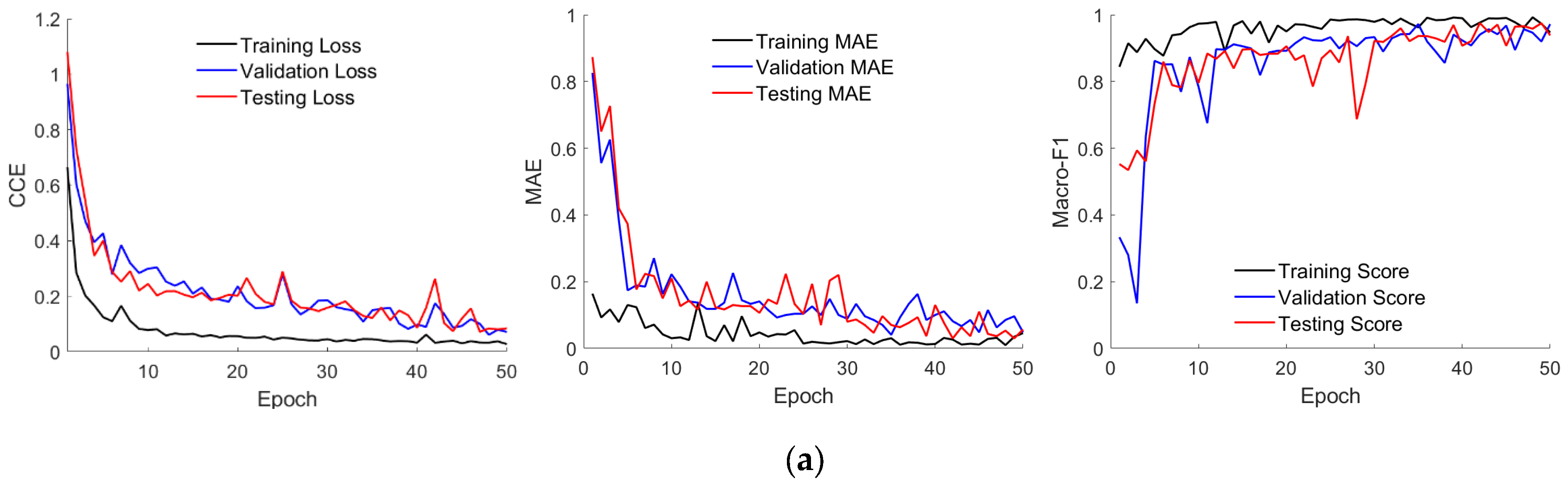
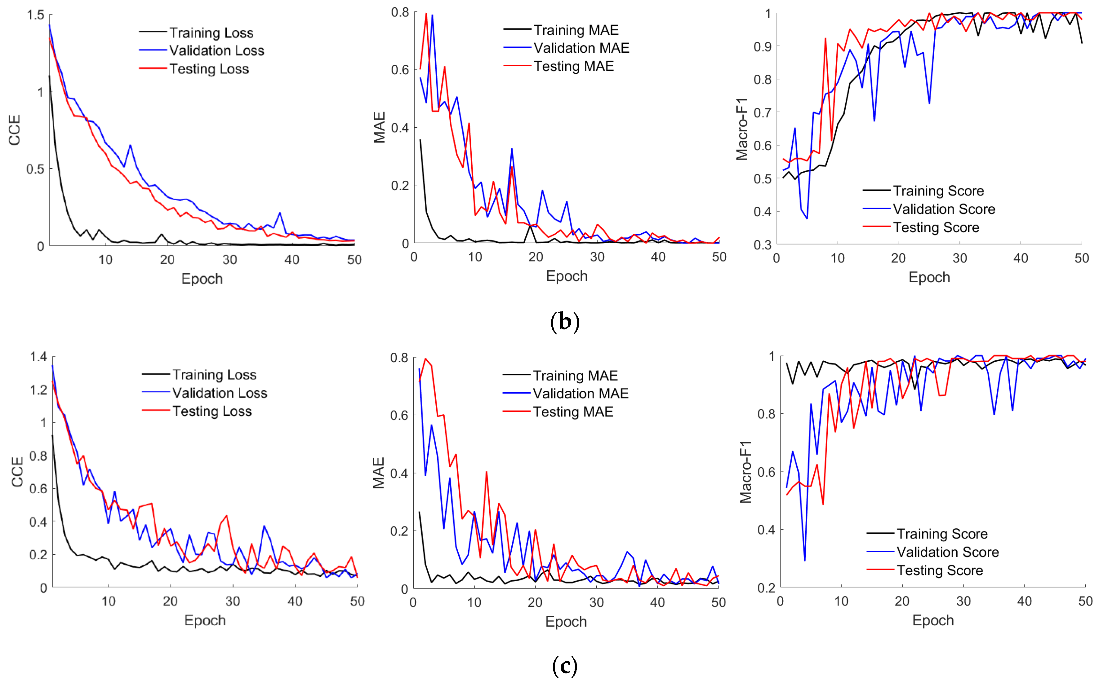
3.1.2. Performance Testing of Models

• DBN performance tests

The performance test mainly includes:

(1)

Comparing the feature learning ability of the three models in the face of different data samples through a single training;

(2)

Observing the prediction performance of the three models on different datasets after multiple training and testing by using a 10-fold cross-validation test.

Test 1: After 100 epochs of pre-training and 50 epochs of reverse fine-tuning, the Loss (CCE), MAE, and Accuracy for the training, validation, and testing of Models I, II, and III are shown in Figure 12.

Test 2: After a 10-fold cross-validation test, the final average test results for Models I, II, and III are shown in

Table 11. Mean of the test results for Model I.

Dataset	MAE	Macro-F1/%	Accuracy/%	Time/s
Training	0.0193	98.38	98.84	0.00809
Validation	0.0156	98.67	99.02	0.00208
Testing	0.0330	97.29	98.13	0.00151

,

Table 12. Mean of the test results for Model II.

Dataset	MAE	Macro-F1/%	Accuracy/%	Time/s
Training	0.0026	99.93	99.74	0.00869
Validation	0.0056	100	99.44	0.00266
Testing	0.0035	100	99.65	0.00242

and

Table 13. Mean of the test results for Model III.

Dataset	MAE	Macro-F1/%	Accuracy/%	Time/s
Training	0.0245	97.35	97.55	0.00641
Validation	0.0361	95.97	96.39	0.00194
Testing	0.0285	94.84	97.15	0.00178

.

Analyzed by the above data, each model shows excellent performance in different deviation pattern recognition tests.

Convergence speed: Analyzed by the Loss curve in Figure 12, Models I and II can converge stably, while Model III has more obvious fluctuation changes during the training process, and the overall convergence speed is slower.

Prediction speed: In Table 11, Table 12 and Table 13, time is the sum of prediction time for all data in the dataset. The average time taken for each data sample in the training of Models I, II, and III is 3.33 $\mathsf{\mu }\mathrm{s}$, 3.58 $\mathsf{\mu }\mathrm{s}$, and 2.64 $\mathsf{\mu }\mathrm{s}$; the average time taken for each sample of data in validation is 7.7 $\mathsf{\mu }\mathrm{s}$, 9.85 $\mathsf{\mu }\mathrm{s}$, and 7.19 $\mathsf{\mu }\mathrm{s}$; the average time taken for each sample of data in testing is 5.03 $\mathsf{\mu }\mathrm{s}$, 8.06 $\mathsf{\mu }\mathrm{s}$, and 5.93 $\mathsf{\mu }\mathrm{s}$. The time consumed, as mentioned above, will not affect the normal operation of the system in comparison with the high-frequency data of the rice transplanter navigation system, and the deviation pattern can be identified very quickly.

Generalization ability: As analyzed by the curves in Figure 12, with the increase in the epoch, the changing trend of the training, validation, and testing is gradually consistent. Combined with the data analysis in Table 11, Table 12 and Table 13, the models have good stability, accuracy, and very fast prediction speed, showing strong generalization ability.

Differences between models: Combining the analysis of figures and tables and comparing the results of Models I, II, and III in the two tests, although the performance of all three models is excellent, the stability and prediction accuracy of Model III are relatively poor.

Difference analysis: There are some differences in the performance of the three models; as analyzed by Section 2.2.1 and Section 2.2.2, the linear correlation between the data features and labels of models I and II is higher, and the difference characteristics between different labeled data are significant. The feature structure of Model III is relatively fuzzier, the feature deviation between different labeled data is smaller, and the weight update rate for hidden features is lower, so the final generated model has poorer discrimination performance.

2.

Comparative validation tests of different deep learning methods

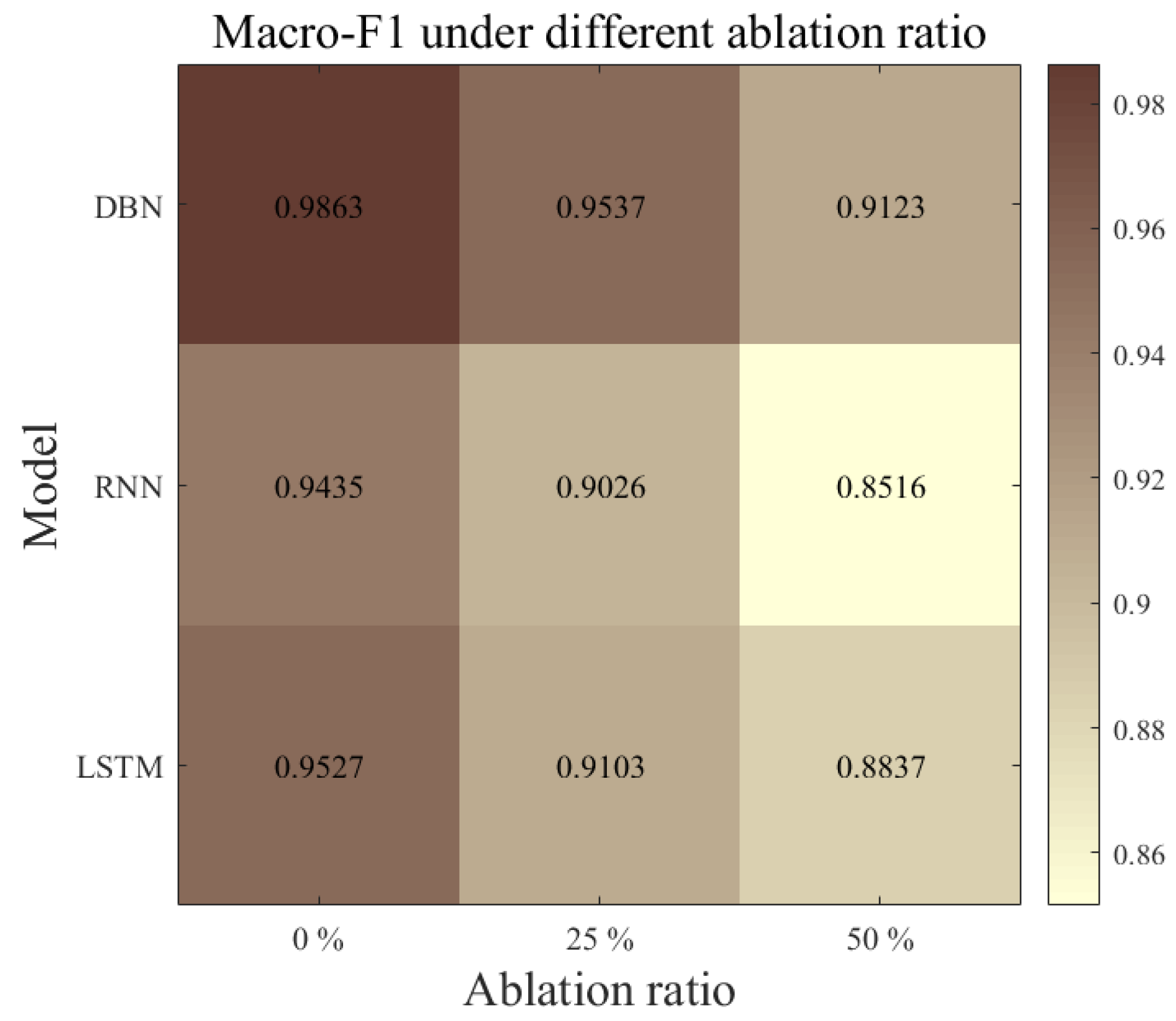
In order to verify the validity and superiority of the present method, this study refers to the traditional classification prediction methods and constructs Recurrent Neural Network (RNN) and Long Short-Term Memory (LSTM) [28] for predicting the data under each deviation pattern and compares them with this study.

Among them, through careful tuning of the hyperparameters, we determined the optimal performance parameters for each model: the structure of RNN is configured as 3 layers of 128 nodes, with a learning rate of 0.05 and a batch size set to 10; the structure of LSTM is configured as 2 layers of 128 nodes, with a learning rate of 0.05 and a batch size set to 30. The two models incorporate a learning-rate decaying strategy.

Models I, II, and III were trained for each of DBN, RNN, LSTM, and MAE, and Macro-F1 and Accuracy were used as performance metrics.

Table 14. Test results of DBN, RNN, and LSTM.

Indicator	Model	DBN	RNN	LSTM
MAE	I	0.0236	0.0967	0.0758
	II	0.0038	0.0235	0.0186
	III	0.0274	0.1694	0.0657
Macro-F1/%	I	98.56	93.57	94.58
	II	99.85	96.96	98.50
	III	95.34	90.36	93.67
Accuracy/%	I	99.02	92.46	92.35
	II	99.58	96.81	98.34
	III	97.44	89.42	92.66

shows the data of the combined prediction performance metrics of various deep learning algorithms for each deviation pattern.

By data analysis, the overall performance metrics of the models constructed using the DBN approach are better than RNN and LSTM, with better discrimination performance, model variability, and accuracy in the three deviant morphology scenarios.

However, DBN, RNN, and LSTM all show variability between Models I, II, and III trained in different deviation morphology scenarios. The performance of Model III of DBN and RNN is more obvious compared to Models I and II, which is in line with the pattern described in the previous section. The performance of Models I and III of LSTM is basically the same, and the LSTM is more sensitive to the transient features’ extraction ability than RNN.

3.

An ablation study of different deep learning methods

Further, in order to compare the robustness of various types of deep learning methods, ablation comparison tests are carried out for DBN, RNN, and LSTM in the scenario of Model I. Since the internal structure of each method is different, a proportional reduction method is used for the ablation level: for DBN, RNN, and LSTM, the number of nodes in each layer is reduced in the proportion of 0%, 25%, and 50% without changing other hyperparameters.

In order to comprehensively evaluate the performance of the three deep learning methods, Macro-F1 is used as the evaluation index, and finally, the variation in the recognition performance of each method is shown in Figure 13.

The comparative result of Figure 13 is analyzed to show that the Macro-F1 values of DBN, RNN, and LSTM show inconsistent differences at different ablation levels. The colors in the figure are from dark to light, indicating that the Macro-F1 values are from high to low. As can be seen from the figure, the Macro-F1 value of DBN decreases from 0.9863 to 0.9123 under different ablation levels but shows the most stable and excellent performance among the three deep learning methods.

All the above performance tests show that the DBN’s excellent extraction ability for hidden features, generalization ability, and extremely fast prediction speed can adapt to the application scenario of the high-frequency and complex environment of a rice transplanter navigation system.

3.2. Simulation Test of Adaptive Control Method Based on Deviation Pattern Identification

3.2.1. Experimental Design

• Test conditions

Forward velocity $v=0.8 \mathrm{m}/\mathrm{s}$, initial heading deviation 0°, initial position deviation 0 m, add positioning noise and steering noise, simulation duration 90 s, sampling time 0.05 s, straight path tracking.

Three cycles are set up to induce different degrees of oscillation in the 7th–10th s of each cycle and different degrees of sideslip in the 25th–26th s.

2.

Control strategy

In practical applications and simulation tests, navigation control deviations are transient, but their subsequent effects on the system are persistent. In order to effectively suppress the effect of transient deviation on the system, the modulation action time is extended after the activation of the sub-regulator according to the degree of oscillation or sideslip, with the logic as shown in (31).

$$\begin{gathered} if \mathit{N}\mathit{a}\mathit{v}\mathit{S}\mathit{t}\mathit{a}\mathit{t}\mathit{e}==\mathit{O}\mathit{s}\mathit{c} \\ { \mathit{T}}_{\mathit{d}\mathit{e}\mathit{l}\mathit{a}\mathit{y}}={\mathit{d}\mathit{e}\mathit{g}}_{\mathit{o}\mathit{c}\mathit{s}} \\ elseif \mathit{N}\mathit{a}\mathit{v}\mathit{S}\mathit{t}\mathit{a}\mathit{t}\mathit{e}==\mathit{S}\mathit{l}\mathit{i}\mathit{p} \\ { \mathit{T}}_{\mathit{d}\mathit{e}\mathit{l}\mathit{a}\mathit{y}}={\mathit{d}\mathit{e}\mathit{g}}_{\mathit{s}\mathit{l}\mathit{i}\mathit{p}} \\ end \end{gathered}$$

(31)

where $\mathit{N}\mathit{a}\mathit{v}\mathit{S}\mathit{t}\mathit{a}\mathit{t}\mathit{e}$ is the anomaly pattern recognized by Model One, $\mathit{O}\mathit{s}\mathit{c}$ is the oscillation state, $\mathit{S}\mathit{l}\mathit{i}\mathit{p}$ is the sideslip state, and ${\mathit{T}}_{\mathit{d}\mathit{e}\mathit{l}\mathit{a}\mathit{y}}$ is the action time of the control strategy.

When the Model One identified that there is a path tracking deviation, the main regulator and the sub-regulator work together to regulate it. The logic is implemented as in (32).

$$\begin{gathered} if {\mathit{T}}_{\mathit{d}\mathit{e}\mathit{l}\mathit{a}\mathit{y}}-- \\ if \mathit{N}\mathit{a}\mathit{v}\mathit{S}\mathit{t}\mathit{a}\mathit{t}\mathit{e}==\mathit{O}\mathit{s}\mathit{c} \\ { \mathit{f}}_{\mathit{s}\mathit{u}\mathit{b}}=\mathit{A}·{\mathit{d}\mathit{e}\mathit{g}}_{\mathit{o}\mathit{c}\mathit{s}} \\ elseif \mathit{N}\mathit{a}\mathit{v}\mathit{S}\mathit{t}\mathit{a}\mathit{t}\mathit{e}==\mathit{S}\mathit{l}\mathit{i}\mathit{p} \\ { \mathit{f}}_{\mathit{s}\mathit{u}\mathit{b}}=\mathit{B}·{\mathit{d}\mathit{e}\mathit{g}}_{\mathit{s}\mathit{l}\mathit{i}\mathit{p}} \\ end \\ { \mathit{f}}_{\mathit{a}\mathit{l}\mathit{l}}={\mathit{f}}_{\mathit{m}\mathit{a}\mathit{i}\mathit{n}}+{\mathit{f}}_{\mathit{s}\mathit{u}\mathit{b}} \\ end \end{gathered}$$

(32)

3.

Test group setup

The two groups, adaptive and static preview distances, are control tests, as shown in

Table 15. Test groups and description.

	A	B	Experimental Purpose
Adaptive preview distance	0.288	0.992	Dynamic preview distance, when a deviation is identified, until the deviation is over.
Static preview distance	NaN	NaN	Static preview distance: 1 m.

.

3.2.2. Test Results

In order to clearly demonstrate the path tracking curves for the adaptive and static preview distances, the complete test cycle is split into three segments of 0–30 s, 30–60 s, and 60–90 s here, as shown in Figure 14.

The results of the path tracking curve for each time segment are shown in

Table 16. Lateral deviation of test.

	Maximum Absolute Lateral Deviation/m			Mean Absolute Lateral Deviation/m			Root Mean Square Lateral Deviation/m
	0~30 s	30~60 s	60~90 s	0~30 s	30~60 s	60~90 s	0~30 s	30~60 s	60~90 s
Static preview distance	0.0642	0.117	0.192	0.0121	0.0232	0.0271	0.0189	0.0346	0.0476
Adaptive preview distance	0.0660	0.0713	0.115	0.0114	0.0146	0.0158	0.0178	0.0205	0.0265

.

From the tracking curves, it can be seen that when the system tracking control deviation occurs, the dynamic preview distance control strategy can quickly and effectively inhibit the system oscillation and sideslip deviation, whereas the static preview distance control strategy is more ineffective in inhibiting the deviation, and it takes a longer time for the system to regain the stable state.

From the lateral deviation data, it can be seen that in the test scenarios of mild deviation (0~30 s), moderate deviation (30~60 s), and severe deviation (60~90 s), the control strategy with adaptive preview distance, compared with static preview distance, has a maximum absolute lateral deviation, MAE and RMSE that are all lower, which fully demonstrates that the former can significantly improve the stability, responsiveness and anti-disturbance ability of the rice transplanter navigation control and the regulation ability in the face of disturbing situations.

As verified by the above experiments, the control method proposed in this study can significantly inhibit the oscillations of the rice transplanter navigation system due to sideslip and multi-factor error coupling, and the design method of the controller is reasonable.

4. Discussion

4.1. Conclusions

In this study, we propose an adaptive preview distance control method based on the deviation suppression strategy of rice transplanter navigation, and the performance is verified by simulation tests.

In the deviation pattern recognition test, the two-stage DBN-based model deployment method has excellent feature learning capability for application scenarios with inconsistent feature tendencies. In the DBN performance test, the method shows very excellent prediction accuracy, stability, and fast prediction speed, with prediction accuracies higher than 96% in different scenarios; in the deep learning method comparison test, DBN shows a stronger feature learning capability compared to RNN and LSTM; and in the ablation study, DBN shows a better structural stability. Combining all these experimental analyses, the DBN-based deviation pattern identification method proposed in this study has strong generalization ability, excellent prediction accuracy, good stability, and very fast identification speed, which can satisfy the application scenario of rice-planting machine navigation.

In the straight path navigation control test, compared with the optimal preview point method [18], both of them are based on the principle of optimizing the preview distance to improve the navigation control performance and have very excellent navigation control performance. However, the optimal preview point method does not analyze the deviation suppression ability in the case of perturbation. Compared with the heading error rate method [29], the control method proposed in this study has faster convergence for transient deviations. Compared with the static preview distance, it improves the path tracking accuracy by 5.79%, 37.07%, and 41.70%, respectively, in different levels of deviation test scenarios.

In conclusion, the adaptive preview distance control strategy proposed in this study has more significant performance advantages for rice transplanter navigation control with complex perturbation variables.

4.2. Outlook

The adaptive preview distance control method proposed in this study can effectively suppress the transient perturbation bias of rice transplanter navigation.

Although the research object is specific (2ZGQ-80D Yangma rice transplanter), the method can be applied to most of the high-speed ride-on rice transplanters relying on front-wheel steering due to the relatively consistent structure, scenarios, and control laws of the rice transplanter navigation and control system. However, the current research has limitations and challenges.

(1)

In the navigation control scenario of the non-straight path, the deviation pattern of the rice transplanter is more complicated, which is a considerable challenge for feature extraction and pattern identification.

(2)

In the DBN model training, the training process and performance of Model Three on the identification of the degree of sideslip deviation are still a bit different compared with the other two models, and the reasons for the analysis are roughly as follows: ① The complexity of the data features is higher; ② the setting of the training parameters of the model is not good. The model performance can be optimized by adding the optimization algorithm to find the suitable training parameters.

(3)

The steering control lag time $\tau$ of the main controller mentioned in this study is difficult to obtain, and a more in-depth study based on the lag time will be carried out subsequently.

(4)

For the above research, we will subsequently construct a complete and efficient adaptive pre-aiming control algorithm in a rice transplanter navigation system through hardware development, model deployment, and algorithm transplantation and test the performance of the algorithm in real products.

References

1. Wei, W.; Xiao, M.; Duan, W.; Wang, H.; Zhu, Y.; Zhai, C.; Geng, G. Research Progress on Autonomous Operation Technology for Agricultural Equipment in Large Fields. Agriculture 2024, 14, 1473. [Google Scholar] [CrossRef]
2. Yao, Z.; Zhao, C.; Zhang, T. Agricultural machinery automatic navigation technology. iScience 2024, 27, 108714. [Google Scholar] [CrossRef] [PubMed]
3. Yin, X.; Wang, Y.; Chen, Y.; Jin, C.; Du, J. Development of autonomous navigation controller for agricultural vehicles. Int. J. Agric. Biol. Eng. 2020, 13, 70–76. [Google Scholar] [CrossRef]
4. Rankin, A.L.; Crane, C.D., III; Armstrong, D.G., II. Evaluating a PID, pure pursuit, and weighted steering controller for an autonomous land vehicle. In Mobile Robots XII, Proceedings of the Intelligent Systems and Advanced Manufacturing, Pittsburgh, PA, USA, 14–17 October 1997; Gage, D.W., Ed.; SPIE: Bellingham, WA, USA, 1998; pp. 1–12. [Google Scholar] [CrossRef]
5. Snider, J.M. Automatic Steering Methods for Autonomous Automobile Path Tracking; Technical Report, no. CMU-RITR-09-08; Robotics Institute: Pittsburgh, PA, USA, 2009. [Google Scholar]
6. Corno, M.; Panzani, G.; Roselli, F.; Giorelli, M.; Azzolini, D.; Savaresi, S.M. An LPV Approach to Autonomous Vehicle Path Tracking in the Presence of Steering Actuation Nonlinearities. IEEE Trans. Contr. Syst. Technol. 2021, 29, 1766–1774. [Google Scholar] [CrossRef]
7. Qin, Z.; Chen, L.; Hu, M.; Chen, X. A Lateral and Longitudinal Dynamics Control Framework of Autonomous Vehicles Based on Multi-Parameter Joint Estimation. IEEE Trans. Veh. Technol. 2022, 71, 5837–5852. [Google Scholar] [CrossRef]
8. Liu, H.; Sun, J.; Cheng, K.W.E. A Two-Layer Model Predictive Path-Tracking Control With Curvature Adaptive Method for High-Speed Autonomous Driving. IEEE Access 2023, 11, 89228–89239. [Google Scholar] [CrossRef]
9. Liu, W.; Hua, M.; Deng, Z.; Meng, Z.; Huang, Y.; Hu, C.; Song, S.; Gao, L.; Liu, C.; Shuai, B.; et al. A Systematic Survey of Control Techniques and Applications in Connected and Automated Vehicles. IEEE Internet Things J. 2023, 10, 21892–21916. [Google Scholar] [CrossRef]
10. Xia, Q.; Chen, P.; Xu, G.; Sun, H.; Li, L.; Yu, G. Adaptive Path-Tracking Controller Embedded With Reinforcement Learning and Preview Model for Autonomous Driving. IEEE Trans. Veh. Technol. 2024, 1–15. [Google Scholar] [CrossRef]
11. Hazem, Z.B.; Bingül, Z. A comparative study of anti-swing radial basis neural-fuzzy LQR controller for multi-degree-of-freedom rotary pendulum systems. Neural Comput. Appl. 2023, 35, 17397–17413. [Google Scholar] [CrossRef]
12. Wu, X.; Fang, P.; Liu, X.; Liu, M.; Huang, P.; Duan, X.; Huang, D.; Liu, Z. AM-UNet: Field Ridge Segmentation of Paddy Field Images Based on an Improved MultiResUNet Network. Agriculture 2024, 14, 637. [Google Scholar] [CrossRef]
13. Mahendran, N.; Vincent, P.M.D.R. Deep belief network-based approach for detecting Alzheimer’s disease using the multi-omics data. Comput. Struct. Biotechnol. J. 2023, 21, 1651–1660. [Google Scholar] [CrossRef] [PubMed]
14. Wang, B.; Tan, Z.; Sheng, W.; Liu, Z.; Wu, X.; Ma, L.; Li, Z. Identification of Groundwater Contamination Sources Based on a Deep Belief Neural Network. Water 2024, 16, 2449. [Google Scholar] [CrossRef]
15. Han, X.; Kim, H.-J.; Jeon, C.W.; Moon, H.C.; Kim, J.H.; Yi, S.Y. Application of a 3D tractor-driving simulator for slip estimation-based path-tracking control of auto-guided tillage operation. Biosyst. Eng. 2019, 178, 70–85. [Google Scholar] [CrossRef]
16. Han, X.-Z.; Kim, H.-J.; Moon, H.-C.; Woo, H.-J.; Kim, J.-H.; Kim, Y.-J. Development of a Path Generation and Tracking Algorithm for a Korean Auto-guidance Tillage Tractor. J. Biosyst. Eng. 2013, 38, 1–8. [Google Scholar] [CrossRef]
17. Han, X.Z.; Kim, H.J.; Kim, J.Y.; Yi, S.Y.; Moon, H.C.; Kim, J.H.; Kim, Y.J. Path-tracking simulation and field tests for an auto-guidance tillage tractor for a paddy field. Comput. Electron. Agric. 2015, 112, 161–171. [Google Scholar] [CrossRef]
18. Yang, Y.; Li, Y.; Wen, X.; Zhang, G.; Ma, Q.; Cheng, S.; Qi, J.; Xu, L.; Chen, L. An optimal goal point determination algorithm for automatic navigation of agricultural machinery: Improving the tracking accuracy of the Pure Pursuit algorithm. Comput. Electron. Agric. 2022, 194, 106760. [Google Scholar] [CrossRef]
19. Wang, H.; Wang, G.; Luo, X.; Zhang, Z.; Gao, Y.; He, J.; Yue, B. Path Tracking Control Method of Agricultural Machine Navigation based on Aiming Pursuit Model. Trans. Chin. Soc. Agric. Eng. Trans. CSAE 2019, 35, 11–19. [Google Scholar] [CrossRef]
20. Na’aim, M.Z.B.M.; Manaf, M.B.A. Establishment of control points using GNSS-RTK technique. E3S Web Conf. 2024, 479, 02001. [Google Scholar] [CrossRef]
21. Wang, S.; Dong, X.; Liu, G.; Gao, M.; Xiao, G.; Zhao, W.; Lv, D. GNSS RTK/UWB/DBA Fusion Positioning Method and Its Performance Evaluation. Remote Sens. 2022, 14, 5928. [Google Scholar] [CrossRef]
22. He, J.; Zhu, J.; Luo, X.; Zhang, Z.; Hu, L.; Gao, Y. Design of Steering Control System for Rice Transplanter Equipped with Steering Wheel-like Motor. Trans. Chin. Soc. Agric. Eng. Trans. CSAE 2019, 35, 10–17. [Google Scholar] [CrossRef]
23. Wang, H.; Hu, J.; Gao, L. Compensation Model for Measurement Error of Wheel Turning Angle in Agricultural Vehicle Guidance. Trans. Chin. Soc. Agric. Mach. 2014, 45, 33–37. [Google Scholar] [CrossRef]
24. Zhang, Z.; Wang, G.; Luo, X.; He, J.; Wang, J.; Wang, H. Detection Method of Steering Wheel Angle for Tractor Automatic Driving. Trans. Chin. Soc. Agric. Mach. 2019, 50, 352–357. [Google Scholar] [CrossRef]
25. Hinton, G.E.; Osindero, S.; Teh, Y.-W. A Fast Learning Algorithm for Deep Belief Nets. Neural Comput. 2006, 18, 1527–1554. [Google Scholar] [CrossRef] [PubMed]
26. Le Roux, N.; Bengio, Y. Representational Power of Restricted Boltzmann Machines and Deep Belief Networks. Neural Comput. 2008, 20, 1631–1649. [Google Scholar] [CrossRef]
27. Chu, H.; Pei, H.; Si, X.-S.; Du, D.-B.; Pang, Z.-N.; Wang, X. A Prognostic Model Based on DBN and Diffusion Process for Degrading Bearing. IEEE Trans. Ind. Electron. 2020, 67, 8767–8777. [Google Scholar] [CrossRef]
28. Sherstinsky, A. Fundamentals of Recurrent Neural Network (RNN) and Long Short-Term Memory (LSTM) network. Phys. D Nonlinear Phenom. 2020, 404, 132306. [Google Scholar] [CrossRef]
29. Wang, L.; Chen, Z.; Zhu, W. An improved pure pursuit path tracking control method based on heading error rate. Ind. Robot. 2022, 49, 973–980. [Google Scholar] [CrossRef]
Figure 1. The overall flowchart.
Applsci 15 00790 g001
Figure 2. The overall structure of the simulation platform.
Applsci 15 00790 g002
Figure 3. Kinematic model of rice transplanter (sideslip perturbation).
Applsci 15 00790 g003
Figure 4. Preview geometry model.
Applsci 15 00790 g004
Figure 5. Structure of DBN.
Applsci 15 00790 g005
Figure 6. Structure of RBM.
Applsci 15 00790 g006
Figure 7. Workflow of each model.
Applsci 15 00790 g007
Figure 8. Dataset acquisition process.
Applsci 15 00790 g008
Figure 9. Workflow of the adaptive preview control algorithm.
Applsci 15 00790 g009
Figure 10. Control curve for actively induced path-tracking deviations.
Applsci 15 00790 g010
Figure 11. Response surface of the Equation (26): color from orange to blue indicate D e c r t e s t from high to low.
Applsci 15 00790 g011
Figure 12. Loss, MAE and Macro-F1 of DBN: (a) Model I; (b) Model II; (c) Model III.
Applsci 15 00790 g012aApplsci 15 00790 g012b
Figure 13. Effects of DBN, RNN, and LSTM on Macro-F1 at different ablation levels.
Applsci 15 00790 g013
Figure 14. Comparison of path-tracking states: (a) 0~30 s; (b) 30~60 s; (c) 60~90 s.
Applsci 15 00790 g014