Improved Honey Badger Algorithm and Its Application to K-Means Clustering

Abstract

As big data continues to evolve, cluster analysis still has a place. Among them, the K-means algorithm is the most widely used method in the field of clustering, which can cause unstable clustering results due to the random selection of the initial clustering center of mass. In this paper, an improved honey badger optimization algorithm is proposed: (1) The population is initialized using sin chaos to make the population uniformly distributed. (2) The density factor is improved to enhance the optimization accuracy of the population. (3) A nonlinear inertia weight factor is introduced to prevent honey badger individuals from relying on the behavior of past individuals during position updating. (4) To improve the diversity of solutions, random opposition learning is performed on the optimal individuals. The improved algorithm outperforms the comparison algorithm in terms of performance through experiments on 23 benchmark test functions. Finally, in this paper, the improved algorithm is applied to K-means clustering and experiments are conducted on three data sets from the UCI data set. The results show that the improved honey badger optimized K-means algorithm improves the clustering effect over the traditional K-means algorithm.

1. Introduction

Cluster analysis, an unsupervised learning technique in data mining, discovers the connections between data by organizing the data into distinct groups based on their similarities [1,2]. K-means [3] has found extensive application across various domains, including image segmentation [4], data mining [5], customer segmentation [6], and pattern recognition [7], among others. The K-means algorithm obtains clustering results by minimizing the squared error within the clusters and randomly selecting the center of mass position during the iteration process. Despite its widespread use, the K-means algorithm has notable limitations. Its widespread use notwithstanding, the K-means method has some drawbacks, most notably its sensitivity to the initial cluster center selection, which may lead to less-than-ideal results. Additionally, the algorithm struggles with handling complex data sets [8,9,10]. These defects seriously affect the effectiveness of the algorithm.

As a result, optimizing the initial cluster centers in K-means has become a crucial focus for enhancing the accuracy of clustering analysis. In recent years, the intelligent optimization algorithm, as a meta-heuristic algorithm of sorts, has gradually come into the public’s view. Numerous researchers have discovered that swarm intelligence algorithms can successfully make up for the K-means algorithm’s drawbacks. Common algorithms include the Grasshopper Optimisation Algorithm [11], Firefly Algorithm [12], Flower Pollination Algorithm [13], etc. Such algorithms help to obtain a better initial center of mass during K-means clustering by modeling the communication and cooperation between groups of organisms. Bai L et al. [14] proposed an artificial fish swarming algorithm based on an improved quantum revolving door. By dynamically adjusting the rotation angle of the quantum rotating gate, the accuracy and speed of the next generation updating direction were improved. The algorithm was applied to the K-means clustering method, leading to enhanced clustering accuracy. Xie H [15] proposed two variations of the firefly algorithm, which enhances the search range and search scale of the firefly and solves the stubborn problem of K-means algorithm. The improved firefly algorithm can obtain better clustering center and improve the clustering effect. With the k-means algorithm’s stubborn problem, the improved firefly algorithm can obtain a better clustering center to improve the clustering effect. Huang P [16], in order to solve the clustering problem, introduced a differential evolution strategy to the initial population of the Honey Badger Algorithm, introduced the equalization pooling technique into the updating of the position at the same time, and finally tested the clustering effect on ten benchmark test sets, which proved its superiority in clustering. Jiang S [17] introduced nonlinear inertia weights into the Flower Pollination Algorithm, as well as Cauchy variation in the optimal solution, and finally applied the improved Flower Pollination Algorithm to K-means clustering and obtained a better clustering effect. Li Y [18] and others proposed an adaptive particle swarm algorithm for optimizing the clustering centers so as to avoid the dependence of the K-means algorithm on the initial clustering centers, which was finally applied to customer segmentation. These algorithms have the ability to jump out of local optimal solutions through population initialization and iterative location updates, thus overcoming the limitations of k-means. Although the flaws of the algorithm have been refined, there are still some shortcomings, such as the chosen meta-heuristic algorithms needing to regulate the parameters, as well as the fact that they are computationally intensive and have high time complexity.

The Honey Badger Algorithm is relatively simple to implement and has less parameter tuning compared to other algorithms. The Honey Badger Algorithm (HBA) [19], introduced by Hashim FA et al. in 2022, is a type of meta-heuristic algorithm. The algorithm builds a mathematical model based on honey badger’s predatory behavior, which includes the behaviors of self-predation and cooperation with other organisms. The Honey Badger Algorithm has an extremely strong global search capability, which facilitates a seamless shift among searching on a global scale and searching locally with a short search time, and performs well in many application problems, especially in solving complex problems.

Many researchers have enhanced the Honey Badger Algorithm and implemented it across various domains since its proposal thanks to its simple structure and fast search speed. Han E et al. [20] proposed an improved HBA to optimize modeling proton exchange membrane fuel cells by using oppositional learning and chaotic mechanisms in the improved algorithm. Chen Y et al. [21] used the HBA to solve the optimization of multi-objectives and applied the HBA to the integrated photovoltaic/extended infiltration/battery system optimization. Arutchelvan K et al. [22] proposed a clustering and routing planning scheme for wireless sensor networks based on the Honey Badger Algorithm. The newly proposed model has the longest lifetime compared to the existing techniques. Song Y et al. [23] combined HBA based on the set of good points with the Distance Vector-Hop (DV-Hop) algorithm to solve the problem of insufficient localization accuracy of the traditional DV-Hop algorithm and to prevent the algorithm from converging to a local optimum. Hu G et al. [24] added a segmental optimal decrement neighborhood and a horizontal hybridization strategy with strategic adaptability to HBA and applied the improved algorithm to unmanned aerial vehicle path planning to obtain a more feasible and efficient path. Hussien A.G. et al. [25] combined the advantages of HBA and the Artificial Gorilla Troops Optimizer to enhance the development ability of the algorithm, and the hybrid algorithm was applied to Bot problems to improve the performance and efficiency of the cloud computing system. Fathy A et al. [26] proposed a microgrid energy management scheme based on HBA considering the advantages of HBA in addressing intricate challenges, and finally improved the operation efficiency of the microgrid.

The Honey Badger Algorithm has inherent limitations, encompassing protracted convergence and a propensity to succumb to local optimal solutions [27]. Moreover, the applications of this algorithm in data clustering tasks are still relatively few, so this manuscript introduces a refined iteration of the Honey Badger Algorithm, termed the Improved Honey Badger Algorithm (IHBA). The IHBA is then applied to K-means clustering. The key contributions of this study can be summarized as follows:

(1)

A sin chaotic strategy for honey badger populations is introduced to ensure that the population is uniformly distributed throughout the search space.

(2)

Improved density factor. This improvement accelerates the rate of convergence.

(3)

Nonlinear inertia weights are introduced in position updating, promoting a smooth transition in exploration and development.

(4)

Reverse learning of optimal individuals to increase population diversity and refine the algorithm to escape from local optima.

(5)

The enhanced algorithm is rigorously assessed through the application of 23 benchmark test functions. Additionally, the clustering analysis problem is addressed with the IHBA proposed in this study, which produces superior clustering results on three UCI test data sets.

The organization of this paper is delineated as follows: Section 2 elucidates the foundational principles underlying the Honey Badger Algorithm. In Section 3, we present an enhanced strategy designed to rectify the inherent limitations associated with the Honey Badger Algorithm. Section 4 meticulously delineates the amalgamation of the K-means algorithm and the Honey Badger Algorithm. Section 5 presents a comprehensive analysis of the results derived from simulation experiments. Finally, Section 6 offers a succinct summary.

2. Honey Badger Algorithm

Honey badgers rely on two main strategies when searching for food: the “digging mode” and the “honey harvesting mode”. In their excavation endeavors, honey badgers harness their acute olfactory abilities to discern the whereabouts of potential prey. Upon arriving in the vicinity of the prey, honey badgers search the neighborhood and then meticulously select an optimal location to excavate and seize their prey. In the mode of honey harvesting, this creature heeds the guidance of its avian companion, enabling it to precisely locate the hive and procure the honey. The entire procedure can be succinctly encapsulated in the following steps.

2.1. Population Initialization

There is a total of N individual honey badgers. Each honey badger is randomly assigned a position within a certain range by using Equation (1).

$$x_i=l{b}_i+r_1\times (u{b}_i-l{b}_i)$$

(1)

In this formula, $x_i$ denotes the position of the honey badger. The variables $u{b}_i$ and $l{b}_i$ are the upper and lower bounds. $r_1$ is a random number generated in the range of 0 to 1.

2.2. Defining Intensity I

In the context of honey badger predation, the intensity of odor plays a crucial role in determining the hunting efficacy of the honey badger. An increase in odor intensity enhances the honey badger’s ability to hunt effectively. The strength of the odor is influenced by several factors, including the distance between honey badgers and the concentration of their prey. Odor intensity is directly proportional to the concentration of the prey and inversely proportional to the distance from it, adhering to the principles of the inverse square law. as shown in Figure 1.

$$\begin{gathered} I_i=r_2\times {\displaystyle \frac{S}{4\pi d_i^2}} \\ S={(x_i-x_{i+1})}^2 \\ {d}_i=x_{prey}-x_i \end{gathered}$$

(2)

where $S$ is the concentrated intensity of the honey badger, that is, the square of the distance between two honey badger individuals; $d_i$ denotes the distance of the prey from the $i$th honey badger; $x_{prey}$ is the position of the prey, that is, the current optimal position; and $r_2$ is a randomly generated number within the range of 0 to 1.

2.3. Define Density Factor

The density factor plays an important role in the honey badger foraging process, and the density factor gradually decreases over time, thus causing the algorithm’s stochasticity to gradually reduce and realizing a smooth transition from global to local search. The specific equation for the density factor is shown in (3).

$$\alpha =C\times \mathrm{e}\mathrm{x}\mathrm{p}({\displaystyle \frac{-t}{t_{max}}})$$

(3)

where $C$ is a constant taking the value 2; $t$ is the current number of iterations; and $t_{max}$ is the maximum number of iterations.

2.4. Digging Phase

In this model, honey badgers move to the perimeter of the prey according to the effects of odor intensity, distance, and density factor, and then dig around the prey. The trajectory of the movement can be regarded as a cardioid curve as shown in Figure 2. The honey badger’s course of action is modeled through Equation (4).

$$x_{new}=x_{prey}\times \omega +F\times \beta \times I\times x_{prey}+F\times r_3\times \alpha \times d_i\times |\mathrm{c}\mathrm{o}\mathrm{s}(2\pi r_4)\times [1-\cos \left(2\pi r_5\right)\left]\right|$$

(4)

In this equation, $x_{prey}$ denotes the position of the prey, and also represents the current optimal position. $\beta$ indicates the honey badger’s food-locating ability, defaulting to 6. Additionally, $r_3$, $r_4$, and $r_5$ are random variables, each ranging from 0 to 1. F can be altered by taking the value 1 or −1 to change the foraging direction of the honey badger. And the formula for F is shown in Equation (5) as follows:

$$F=\left\{\begin{array}{c}1 r_6\le 0.5\\ -1 else \end{array}\right.$$

(5)

2.5. Honey Phase

In addition to feeding on their own, honey badgers also like to eat honey, but the badgers are unable to locate the hives, so they enter into a partnership with a guide bird, which lead the badgers to the locations of hives. This process can be modeled as Equation (6):

$$x_{new}=x_{prey}+F\times r_7\times \alpha \times d_i$$

(6)

The random number $r_7$ has a value between 0 and 1. The search behavior of honey badgers is influenced by a variety of factors that work together to guide the honey badger towards the vicinity of its prey.

The basic HBA flowchart is shown in Figure 3.

3. Improved Honey Badger Algorithm

The HBA, despite its simplicity and ease of understanding, has notable limitations. At present, the HBA has some problems such as slow convergence speed and low convergence accuracy. To address these issues, this paper proposes improvements to the algorithm from four aspects, with the goal of enhancing its overall optimization performance. In the following sections, the specific strategies for these improvements will be discussed in detail.

3.1. Sin Chaotic Initial Population

In intelligent optimization algorithms, initialization of the individuals in the population is carried out first. HBA adopts the form of a randomly distributed initial population, which may lead to the individuals of the population concentrating in certain regions of the solution space, which in turn leads to a decrease in the accuracy of the solution. Therefore, this paper adopts sin chaos for population initialization to resolve the aforementioned problems. A sin chaos model [28] is a kind of model with an infinite number of mapping folding times in a finite region, possessing stronger chaotic properties as well as ergodicity. Upon the completion of a predetermined number of iterations, the initial population can spread over the entire solution space.

The procedure for initializing the population utilizing sin chaos is outlined as follows:

(1)

N honey badger populations and the position of each individual honey badger are initialized within a D-dimensional space, denoted as $Z_1=\left\{z_1,z_2,\dots z_i\dots ,z_D\right\}$, $i\in [1,D]$;

(2)

Equation (7) is employed to iteratively generate chaotic sequences for each dimension of Z until the remaining N-1 honey badger individuals are produced;

$$\left\{\begin{array}{c}{z}_{n+1}=\sin \left({\displaystyle \frac{2}{z_n}}\right) n=\mathrm{1,2}\dots ,D\\ {-1\le z}_n\le 1 z_n\ne 0\end{array}\right.$$

(7)

where $z_n$ is a sequence of values from −1 to 1. $z_n$ cannot be 0.

(3)

The aforementioned chaotic sequence is mapped to the initial position of an individual honey badger within the search space:

$$x_{iD}=lb+(ub-lb)\times {\displaystyle \frac{1+z_{iD}}{2}}$$

(8)

$lb$ for the lower world, $ub$ for the upper world.

The sin chaotic model leverages its advantageous chaotic properties and traversal capabilities to explore various regions within a finite solution space through multiple periodic iterations. This approach enables the optimization process to encompass a broader solution space, thereby providing rich population information for the subsequent optimization phases of the algorithm.

3.2. Improved Density Factor

The density factor plays a crucial role in regulating the randomness of HBA. In the pre-iteration period, the algorithm requires a comprehensive exploration of the solution space, while at the same time, the density factor takes a large value, which increases the randomness and facilitates the algorithm in executing a comprehensive and far-reaching search. Later in the iteration, the algorithm converges towards the optimal solution, and the density factor diminishes to facilitate the algorithm’s ability to identify the optimal solution within a more confined area.

The original density factor decreases over the course of the iterations, but the decrease is slow and takes a narrow range of values, which can lead to premature convergence of the algorithm and output of poor-quality solutions. Therefore, a new density factor ${\alpha }_1$ is introduced [29]. ${\alpha }_1$ is formulated as shown in Equation (9):

$${\alpha }_1=C-C\times \sin \left({\displaystyle \frac{t}{t_{max}}}\times {\displaystyle \frac{\pi }{2}}\right)+\sigma \times r$$

(9)

where $r$ is a random number obeying a normal distribution and $\sigma$ is the variance of the normal distribution.

As shown in Figure 4, the improved density factor ${\alpha }_1$ decreases more rapidly by the middle of the iteration, which allows IHBA to have a faster convergence rate in the early stage; also, in the late iteration, ${\alpha }_1$ varies less so that the algorithm can perform a full local search. ${\alpha }_1$ also introduces the random number rand and the variance $\sigma$ to enhance the diversity of the solutions of ${\alpha }_1$.

3.3. Nonlinear Inertia Weights

In intelligent optimization algorithms, the nonlinear inertial weight refers to a dynamically adjusted weight that varies in a non-linear manner throughout the optimization process. Particle swarm algorithms have demonstrated that inertia weights reflect the ability of the latter follower to escape from the previous position, as well as that larger inertia weights lead to better global search capabilities, and conversely, smaller inertia weights lead to better local exploitation [30]. In the HBA, the update of the individual location largely depends on the optimal location found in the last iteration. This over-reliance on past optimal solutions can lead to an imbalance between the potential for exploration and the ability for exploitation.

Therefore, nonlinear inertia weights were introduced into the two foraging patterns of honey badgers. The nonlinear inertia weight parameters [31] are shown in Equation (10):

$$\omega ={\displaystyle \frac{1}{1+1.5e^{\frac{10t}{t_{max}}-5}}}-0.1\times r$$

(10)

where $r$ is a random number from 0 to 1; $t$ is the current iteration number; and $t_{max}$ is the maximum iterations.

The HBA’s mining phase (Equation (4)) and honey phase (Equation (6)) are updated to Equations (11) and (12).

$$x_{new}=x_{prey}\times \omega +F\times \beta \times I\times x_{prey}+F\times r_3\times \alpha \times d_i\times |\mathrm{c}\mathrm{o}\mathrm{s}(2\pi r_4)\times [1-\cos \left(2\pi r_5\right)\left]\right|$$

(11)

$$x_{new}=x_{prey}\times \omega +F\times r_7\times \alpha \times d_i$$

(12)

The inertia weight $\omega$ decreases as the quantity of iterations increases. The early inertia weight is relatively large, which means that the improved Honey Badger Algorithm can rely more on the standing of the present individual so as to achieve a thorough global search. As the algorithm progresses, the inertia weight gradually goes down, and the impact between successive generations decreases. The use of nonlinear inertia weights facilitates a balance between global exploration and local exploitation, thereby reducing the time required to approach the optimal solution.

3.4. Perturbation Strategy Based on Random Opposition

Random Opposition-Based Learning can help algorithms to remove local optimal solutions and improve their diversity. By introducing random numbers, the algorithm can explore different directions and angles during the search process. This random performance enhances the diversity of the population and finds better solutions [32,33,34]. The specific formula of Random Opposition-Based Learning is shown in Equation (13).

$$X_{rand}=lb+ub-rand\times X$$

(13)

Here, $X_{rand}$ is a new solution generated after random reverse learning; the value of rand is randomly generated from 0 to 1; and $lb$ and $ub$ are the bounds of the solution space.

Adding the Random Opposition-Based Learning strategy certainly prevents the algorithm from succumbing to a local optimum, but there is no guarantee that the position after perturbation will approach the optimal solution. Therefore, a greedy algorithm [35] is added after Random Opposition-Based Learning to compare the fitness and retain the current optimal solution.

$$X_{best}=\left\{\begin{array}{c}{X}_{rand} f\left(X_{rand}\right)\le f(X_b^{*} )\\ X_b^{*} f\left(X_{rand}\right)\le f(X_b^{*} ) \end{array}\right.$$

(14)

where $X_b^{\mathrm{*}}$ is the original optimal solution.

The IHBA flow diagram is shown in Figure 5.

3.5. Computational Complexity Analysis of IHBA

Time complexity serves as a crucial metric for assessing the efficiency of an algorithm’s solution. Therefore, an analysis of IHBA with respect to its time complexity is conducted. The computational cost of the IHBA can be categorized into four components: the generation of a chaotic initial population, the evaluation of fitness values, position updates, and the computation of inverse solutions. $N$ represents honey badger individuals, $t_{max}$ denotes the maximum number of iterations, and $d$ indicates the dimension. The initial phase of the algorithm encompasses the initialization of population positions, fitness evaluation, and other related processes, resulting in an overall complexity of $O\left(Nd\right)$. The complexity of the algorithm’s operations, including position updating and the calculation of the inverse solution, is $O\left(t_{max}N\right)$. Thus, the overall complexity of IHBA is as in Equation (15).

$$T=O(Nd+t_{max}N)$$

(15)

4. K-Means Algorithm Based on Improved Honey Badger Algorithm

In this study, a K-means algorithm based on the Improved Honey Badger Algorithm (IHBA-KM) is proposed as a way to compensate for the lack of random selection of the center of mass in K-means. IHBA-KM uses the sin chaos method for population initialization, thereby increasing the randomness and diversity of initial clustering centers. By introducing an improved density factor, the algorithm can better adapt to different data distributions. In the process of position updating, nonlinear inertial weights are used to make the search process more balanced. In addition, the incorporation of random opposition-based learning significantly enhances the selection process for clustering centers. Next, this paper will describe the detailed steps of IHBA-KM:

Step 1: Initialization parameters are set: data set $S$, population number $N$, maximum number of iterations $t_{max}$, and cluster number $K$;

Step 2: $K$ data points are selected randomly from the data set to serve as the positions of honey badgers. These data points will be used as candidate cluster centers in the initial stage, and initial locations will be assigned to honey badgers according to different dimensions. The process will be repeated N times, a total of N honey badger individuals will be generated, and then new locations of the honey badgers will be calculated according to Formula (8).

Step 3: According to step 2, there are $2N$ honey badger individuals, including the original solution and the chaotic solution. The data set is clustered, the fitness is assigned, and at the same time, the first $N$ honey badgers are taken as the initial population.

Step 4: The optimal individual and its fitness are discovered;

Step 5: A random number $r$ is generated. $r$ is less than 0.5. The algorithm carries out a global search, uses Formula (11) to update the position, and carries out boundary processing;

Step 6: Otherwise, the algorithm carries out a local search, uses Formula (12) to update the position, and carries out boundary processing;

Step 7: Clustering operations are performed after the location update, and the newly generated cluster center is set to the location updated in step 5 or 6;

Step 8: The current optimal solution is updated, and then the opposition solution is calculated according to Formula (13). The fitness of the opposition solution is compared with the original global optimal solution. The solution with the least fitness is the global optimal solution, and the corresponding position is saved as the best position.

Step 9: Step 5 and Step 6 are repeated until termination conditions are met;

Step 10: Using the optimal solution as the cluster center, the distance from the data points to the clustering center is calculated and the data are assigned to the closest cluster. The optimal solution, location, and clustering results are output.

To summarize the steps above, we provide the pseudo code of IHBA-KM, as shown in Algorithm 1.

Algorithm 1 Pseudo code of IHBA-KM

Initialize the parameters of the algorithm: $S, K, N$$, t_{max}$.

Initialize population location at random positions.

Initialization of the population using the sin chaos.

Cluster data set.

$\mathrm{evaluate} \mathrm{the} \mathrm{fitness} \mathrm{of} \mathrm{every} x_i$$\mathrm{and} \mathrm{give} \mathrm{it} \mathrm{to} f_i$.

$\mathrm{Save} \mathrm{the} \mathrm{best} \mathrm{position} x_{prey}$$\mathrm{and} \mathrm{give} \mathrm{its} \mathrm{fitness} f_{prey}$.

while $t\le$$t_{max}$ do

$\mathrm{Update} \mathrm{the} \mathrm{factor} {\alpha }_1$ using Equation (9).

for $i$ = $1 \mathrm{to} N$ do

Calculate the intensity I using Equation (2).

if $r$ < 0.5 then

Update the new position using Equation (11).

else

Update the new position using Equation (12).

end if

Execute clustering.

Evaluate the new position and assign to fitness.

$\mathrm{Calculate} \mathrm{the} \mathrm{random} \mathrm{reverse} \mathrm{solution} x_{ROBL}$ $\mathrm{using} \mathrm{Equation} \left(13\right) \mathrm{and} \mathrm{assign} \mathrm{to} f_{ROBL}$.

if $f_{ROBL}\le f_i$ then

$x_i=x_{ROBLi}$$\mathrm{and} f_i=f_{ROBLi}$

end if

if $f_{ROBL}\le f_{prey}$ then

$x_{prey}=x_{ROBL}$$\mathrm{and} f_{prey}=f_{ROBL}$

end if

end for

end while

Return $x_{prey}$, $f_{prey}$ and clustering results.

5. Simulation Experiment and Analysis

The initial experiment aimed to evaluate the efficacy of the Particle Swarm Optimization (PSO) [36], Whale Optimization Algorithm (WOA) [37], Artificial Rabbit Optimization (ARO) [38], Spider Wasp Optimization (SWO) [39], HBA, and IHBA on the benchmark function, and then to conduct a detailed comparative analysis based on the results. Specific parameter settings are shown in

Table 1. Parameter settings.

Algorithms	Parameter
PSO	$c_1=c_2=2$$, \omega =0.7$
WOA	$b=0.7$
ARO	-
SWO	$R=0.3$$, Cr=0.2$ $N\_min=20$
HBA	$\beta =6$$, C=2$
IHBA	$\beta =6$$, C=2$

. The second set of experiments applied IHBA to the K-means clustering task. This was compared with HBA and the standard K-means algorithm to evaluate the advantages of IHBA in clustering performance.

5.1. Preparation of Experimental Environment

All experiments conducted in this study were performed on a sophisticated computer system operating under the 64-bit Windows 11 environment. This system was powered by an Intel Core i5-8250U processor and was equipped with a robust 8 GB of RAM, ensuring optimal performance for our research endeavors. The programming language was Python, and the drawing software was MATLAB 2021a and Origin 2021.

In this study, a total of 23 benchmark [40] test functions were chosen to evaluate the performance of the algorithm, as shown in

Table 2. Unimodal functions.

Test Function	Solution Domain	Best	Dimensionality
$F_1\left(x\right)={\sum }_{i=1}^D{x}_i^2$	[−100, 100]	0	30
$F_2\left(x\right)={\sum }_{i=1}^D\left|x_i\right|+{\prod }_{i=1}^D\left|x_i\right|$	[−10, 10]	0	30
$F_3\left(x\right)={\sum }_{i=1}^D{\left({\sum }_{j=1}^i{x}_j\right)}^2$	[−100, 100]	0	30
$F_4\left(x\right)={max}_i\left\{\left|x_i\right|,1\le i\le D\right\}$	[−100, 100]	0	30
$F_5\left(x\right)={\sum }_{i=1}^D\left|x_i\right|$	[−100, 100]	0	30
$F_6\left(x\right)={\sum }_{j=2}^{D-2}\left[{\left(x_{i-1}-10x_i\right)}^2+5{\left(x_{i+1}-x_{i+2}\right)}^2+{\left(x_i-x_{i+1}\right)}^4+10{\left(x_{i-1}-x_{i+2}\right)}^4\right]$	[−4, 5]	0	30
$F_7\left(x\right)={\sum }_{i=1}^{D}i\times x_i^4+random\left[\mathrm{0,1}\right)$	[−1.28, 1.28]	0	30
$F_8\left(x\right)={\sum }_{i=1}^D{\left|x_i\right|}^{i+1}$	[−1, 1]	0	30
$F_9\left(x\right)={\sum }_{i=1}^{D}i{x}_i^2$	[−10, 10]	0	30

,

Table 3. Multimodal functions.

Test Function	Solution Domain	Best	Dimensionality
$F_{10}\left(x\right)={\sum }_{i=1}^D{-x}_i\times \mathrm{s}\mathrm{i}\mathrm{n}\left(\sqrt{\left|x_i\right|}\right)$	[−500, 500]	−418.9829 × D	30
$F_{11}={\sum }_{i=1}^D[x_i^2-10\times \cos \left(2\pi x_i\right)+10]$	[−5.12, 5.12]	0	30
$F_{12}\left(x\right)=x_1^2+{10}^6{\sum }_{i=2}^D{x}_i^2$	[−10, 10]	0	30
$F_{13}={\displaystyle \frac{1}{4000}}{\sum }_{i=1}^D{x}_i^2-{\prod }_{i=1}^D\cos \left({\displaystyle \frac{x_i}{\sqrt{i}}}\right)+1$	[−600, 600]	0	30
$F_{14}\left(x\right)={\sum }_{i=1}^D{x}_i^6[2+sin({\displaystyle \frac{1}{x_i}})]$	[−10, 10]	0	30
$F_{15}\left(x\right)=\sum _{i=1}^D{x}_i^2+{\left(\sum _{i=1}^{D}0.5i{x}_i\right)}^2+{\left(\sum _{i=1}^{D}0.5i{x}_i\right)}^4$	[−5, 10]	0	30
$F_{16}\left(x\right)=0.5+{\displaystyle \frac{\left[{\left(\mathit{sin}\sqrt{{\sum }_{i=1}^D{x}_i^2}\right)}^2-0.5\right]}{{\left[1+0.001\left({\sum }_{i=1}^D{x}_i^2\right)\right]}^2}}$	[−10, 10]	0	30

and

Table 4. Fixed-dimensional functions.

Test Function	Solution Domain	Best	Dimensionality
$F_{17}\left(x\right)=100\sqrt{\left|x_2-0.01x_1^2\right|}+0.01\left|x_1+10\right|$	[−10, 1]	0	2
$F_{18}\left(x\right)=-0.0001{\left(\left|\mathit{sin}\left(x_1\right)\mathit{sin}\left(x_2\right)\mathit{exp}\left(\left|100-{\displaystyle \frac{\sqrt{x_1^2+x_2^2}}{\pi }}\right|\right)\right|+1\right)}^{0.1}$	[−10, 10]	−2.06261	2
$F_{19}\left(x\right)={(2x_1^3{x}_2-x_2^3)}^2+{(6x_1-x_2^2+x_2)}^2$	[−500, 500]	0	2
$F_{20}=0.5+{sin}^2\left(x_1^2-x_2^2\right)-0.5/{[1+0.001\left(x_1^2+x_2^2\right)]}^2$	[−100, 100]	0	2
$F_{21}\left(x\right)=0.26\left(x_1^2+x_2^2\right)-0.48x_1{x}_2$	[−10, 10]	0	2
$F_{22}\left(x\right)=2x_1^2-1.05x_1^4+x_1^6/6+x_1{x}_2+x_2^2$	[−5, 5]	0	2
$F_{23}\left(x\right)=100{\left(x_1^2-x_2\right)}^2+{\left(x_1-1\right)}^2+{\left(x_3-1\right)}^2+90{\left(x_3^2-x_4\right)}^2+10.1\left({\left(x_2-1\right)}^2+{\left(x_4-1\right)}^2\right)+19.8\left(x_2-1\right)\left(x_4-1\right)$	[−10, 10]	0	4

. The test function was divided into three groups: unimodal function (F1–F9), multimodal function (F10–F16), and fixed dimensional function (F17–F23). To ensure fairness, population $N$ = 50, maximum number of iterations $t_{max}$ = 500, and dimension $D$ = 30/200 were set in the experiment. Each algorithm was run independently 30 times, and the mean, optimum, and standard deviation of the 30 runs were recorded. These indicators together evaluated the efficiency, stability and optimization ability of the algorithm.

5.2. Experimental Comparative Analysis of Improved Honey Badger Algorithm

The IHBA and the comparison algorithm were tested at $D$ = 30 and $D$ = 200, respectively, and the test results are shown in

Table 5. Error statistics (average, standard deviation, best) for 30 runs of the IHBA and comparison algorithms on single-peak and multi-peak test functions (D = 30).

Functions	ATR	PSO	WOA	ARO	SWO	HBA	IHBA
F1	Avg	1.40 × 101	7.57 × 10−83	9.08 × 10−59	3.95 × 102	7.28 × 10−147	0
	Std	2.29	4.11 × 10−82	4.97 × 10−58	7.91 × 102	8.43 × 10−146	0
	Best	8.88	1.1 × 10−94	1.27 × 10−71	2.70 × 10−1	6.06 × 10−152	0
F2	Avg	1.64 × 101	1.62 × 10−54	4.14 × 10−33	3.60	7.34 × 10−77	0
	Std	9.10 × 10−1	6.34 × 10−54	1.31 × 10−32	8.22	3.63 × 10−76	0
	Best	1.44 × 101	3.24 × 10−60	4.93 × 10−37	6.39 × 10−3	7.47 × 10−81	0
F3	Avg	5.60 × 101	2.79 × 104	6.43 × 10−47	6.89 × 102	1.23 × 10−99	0
	Std	1.28 × 101	1.11 × 104	2.15 × 10−46	1.35 × 103	5.85 × 10−99	0
	Best	2.90 × 101	8.36 × 103	2.89 × 10−57	9.09 × 102	1.22 × 10−109	0
F4	Avg	1.52	3.54 × 101	2.89 × 10−25	4.15	3.25 × 10−62	0
	Std	1.07 × 101	2.19 × 101	9.77 × 10−25	5.21	6.05 × 10−62	0
	Best	1.31	1.65 × 10−1	2.86 × 10−31	6.59 × 10−3	6.09 × 10−65	0
F5	Avg	1.68 × 101	7.85 × 10−54	2.04 × 10−32	6.54	1.90 × 10−75	0
	Std	1.56	1.58 × 10−53	8.03 × 10−32	9.87	3.27 × 10−75	0
	Best	1.45 × 101	1.25 × 10−57	2.64 × 10−37	3.88 × 10−4	2.25 × 10−78	0
F6	Avg	2.14 × 103	5.78 × 10−89	6.36 × 10−60	7.03 × 101	2.00 × 10−139	1.88 × 10−138
	Std	4.28 × 102	3.04 × 10−88	3.18 × 10−59	1.43 × 102	1.10 × 10−138	1.02 × 10−138
	Best	1.33 × 103	1.0 × 10−99	6.59 × 10−68	1.79 × 10−4	2.25 × 10−147	7.84 × 10−204
F7	Avg	1.03 × 10−1	2.13 × 10−3	5.30 × 10−4	1.32 × 10−1	1.32 × 10−4	6.11 × 10−5
	Std	5.66 × 10−2	2.32 × 10−3	3.23 × 10−4	1.20 × 10−1	5.93 × 10−5	4.76 × 10−5
	Best	3.44 × 10−2	2.47 × 10−5	5.01 × 10−5	7.51 × 10−3	1.30 × 10−5	3.08 × 10−6
F8	Avg	1.73 × 10−5	1.49 × 10−128	4.14 × 10−4	6.71 × 10−4	0	0
	Std	1.60 × 10−5	8.17 × 10−128	2.47 × 10−4	3.20 × 10−3	0	0
	Best	9.70 × 10−7	1.50 × 10−163	8.25 × 10−5	0	0	0
F9	Avg	2.07 × 102	8.83 × 10−84	5.11. × 10−4	1.19 × 102	2.09 × 10−147	0
	Std	2.50 × 101	4.82 × 10−83	4.40 × 10−4	2.70 × 102	5.11 × 10−147	0
	Best	1.79 × 102	7.70 × 10−96	1.67 × 10−6	0	5.67 × 10−154	0
F10	Avg	−6.23 × 103	−5.31 × 103	−1.60 × 104	−3.90 × 103	−8.96 × 103	−1.08 × 104
	Std	9.57 × 102	7.40 × 102	5.19 × 102	3.82 × 102	9.02 × 102	6.01 × 102
	Best	−7.94 × 103	−6.06 × 103	−1.14 × 104	−4.96 × 103	−1.02 × 104	−1.18 × 104
F11	Avg	2.19 × 102	3.79 × 10−15	0	1.60 × 10−5	0	0
	Std	1.29 × 101	1.44 × 1014	0	6.04 × 101	0	0
	Best	1.98 × 102	0	0	1.42 × 103	0	0
F12	Avg	1.37 × 107	1.90 × 10−80	3.46 × 10−55	3.70 × 106	3.33 × 10−136	0
	Std	1.79 × 106	4.16 × 10−79	1.80 × 10−54	1.30 × 107	1.69 × 10−135	0
	Best	1.09 × 107	7.69 × 10−92	4.29 × 10−67	8.11 × 10−1	3.80 × 10−150	0
F13	Avg	6.26 × 10−1	3.98 × 10−3	0	1.44 × 101	0	0
	Std	4.83 × 10−2	2.18 × 10−2	0	5.43 × 101	0	0
	Best	5.57 × 10−1	0	0	4.21 × 10−2	0	0
F14	Avg	2.85	1.62 × 10−148	1.33 × 10−166	4.55	5.31 × 10−68	0
	Std	6.95 × 10−1	7.23 × 10−148	0	1.55 × 101	2.90 × 10−67	0
	Best	1.37	2.82 × 10−183	1.99 × 10−210	0	2.61 × 10−85	0
F15	Avg	3.69 × 101	5.08 × 102	5.18 × 10−32	4.29 × 101	2.73 × 10−67	5.83 × 10−217
	Std	2.81 × 101	1.02 × 102	2.83 × 10−31	7.31 × 101	1.26 × 10−66	0
	Best	4.91	2.62 × 102	2.67 × 10−48	5.98 × 10−2	3.28 × 10−81	5.29 × 10−238
F16	Avg	1.63 × 10−2	1.84 × 10−2	−6.00 × 10−2	5.30 × 10−2	2.24 × 10−3	0
	Std	5.59 × 103	1.74 × 10−2	0	4.17 × 102	5.80 × 10−4	0
	Best	9.59 × 10−3	0	−6.00 × 10−2	9.73 × 10−3	6.78 × 10−5	0

,

Table 6. Error statistics (average, standard deviation, best) for 30 runs of the IHBA and comparison algorithms on single-peak and multi-peak test functions (D = 200).

Functions	ATR	PSO	WOA	ARO	SWO	HBA	IHBA
F1	avg	9.37 × 103	3.55 × 10−82	2.88 × 10−51	2.82 × 103	1.12 × 10−124	0
	std	1.10 × 103	1.15 × 10−81	1.56 × 10−50	5.85 × 103	4.20 × 10−124	0
	best	7.28 × 103	2.35 × 10−91	3.43 × 10−60	7.42 × 10−3	2.60 × 10−129	0
F2	avg	1.94 × 102	2.39 × 10−52	1.67 × 10−29	2.36 × 101	2.49 × 10−67	0
	std	7.26 × 101	1.15 × 10−51	4.85 × 10−29	3.16 × 101	5.96 × 10−67	0
	best	5.60 × 101	2.75 × 10−62	1.29 × 10−33	1.21 × 10−1	4.66 × 10−69	0
F3	avg	5.76 × 104	4.38 × 106	1.04 × 10−37	6.59 × 104	4.97 × 10−77	0
	std	9.64 × 103	1.18 × 106	5.36 × 10−37	1.37 × 105	2.20 × 10−76	0
	best	3.31 × 104	2.39 × 106	3.87 × 10−46	2.54	5.12 × 10−88	0
F4	avg	1.19 × 101	7.87 × 101	2.20 × 10−21	1.37 × 101	1.23 × 10−35	0
	std	1.15	2.15 × 101	3.75 × 10−21	1.86 × 101	2.91 × 10−35	0
	best	9.48	6.63	7.81 × 10−25	3.79 × 10−3	3.40 × 10−38	0
F5	avg	1.32 × 103	1.36 × 10−51	1.53 × 10−29	5.04 × 102	3.98 × 10−66	0
	std	1.96 × 101	3.78 × 10−51	5.33 × 10−29	5.83 × 102	1.26 × 10−65	0
	best	1.09 × 103	3.60 × 10−58	3.38 × 10−33	6.38 × 10−1	4.45 × 10−68	0
F6	avg	2.75 × 104	1.67 × 10−84	9.20 × 10−55	1.19 × 103	6.30 × 10−124	3.01 × 10−132
	std	1.61 × 104	6.27 × 10−84	2.18 × 10−54	3.56 × 103	2.96 × 10−123	9.04 × 10−132
	best	9.10 × 103	2.55 × 10−94	6.29 × 10−62	2.64 × 10−2	1.72 × 10−131	7.05 × 10−182
F7	avg	1.51 × 102	2.17 × 10−3	5.79 × 10−4	4.89	3.09 × 10−4	7.99 × 10−5
	std	1.70 × 102	2.66 × 10−3	4.14 × 10−4	1.67 × 101	2.21 × 10−4	5.89 × 10−5
	best	4.53	4.39 × 10−4	1.36 × 10−5	1.30 × 10−2	6.09 × 10−5	1.00 × 10−5
F8	avg	3.04 × 10−5	7.99 × 10−123	1.02 × 10−123	1.11 × 10−4	1.80 × 10−249	0
	std	3.63 × 10−5	4.37 × 10−122	4.98 × 10−123	3.31 × 10−4	0	0
	best	6.63 × 10−7	8.38 × 10−148	5.22 × 10−143	0	4.74 × 10−283	0
F9	avg	6.38 × 10−4	1.96 × 10−82	2.36 × 10−52	1.82 × 103	1.37 × 10−124	0
	std	1.94 × 10−4	6.01 × 10−82	1.27 × 10−51	4.31 × 10−3	2.00 × 10−24	0
	best	9.91 × 102	2.01 × 10−95	2.59 × 10−60	5.00 × 10−6	1.88 × 10−29	0
F10	avg	−3.55 × 104	−5.62 × 104	−4.00 × 104	−1.04 × 104	−4.45 × 104	−5.30 × 104
	std	4.72 × 103	2.96 × 10−11	1.24 × 103	1.16 × 103	6.10 × 103	6.75 × 103
	best	−4.20 × 104	−5.62 × 104	−4.23 × 10−4	−1.34 × 104	−5.15 × 104	−8.37 × 10−4
F11	avg	1.82 × 103	1.52 × 10−14	0	4.00 × 102	0	0
	std	2.04 × 102	8.30 × 10−14	0	5.47 × 102	0	0
	best	1.42 × 103	0	0	8.99 × 102	0	0
F12	avg	2.26 × 108	2.68 × 10−78	1.60 × 10−49	3.55 × 107	4.34 × 10−116	0
	std	1.49 × 108	1.04 × 10−77	4.28 × 10−49	1.36 × 108	2.33 × 10−115	0
	best	8.78 × 105	7.53 × 10−86	4.20 × 10−58	9.93 × 102	9.93 × 10−129	0
F13	avg	5.57	0	0	2.04 × 101	0	0
	std	4.70 × 10−1	0	0	3.38 × 101	0	0
	best	4.62	0	0.	5.24 × 10−3	0	0
F14	avg	5.39	7.49 × 10−143	1.58 × 10−140	7.06 × 102	0	0
	std	9.11	3.02 × 10−142	8.68 × 10−140	2.52 × 103	0	0
	best	4.41 × 10−1	3.07 × 10−191	9.82 × 10−178	0	0	0
F15	avg	6.71 × 10−3	3.19 × 103	2.86 × 104	3.19 × 105	7.23	8.73 × 10−170
	std	1.52 × 103	2.49 × 102	8.90 × 10−4	1.68 × 106	1.38 × 101	0
	best	3.12 × 103	2.58 × 103	2.31 × 10−14	1.54 × 10−1	3.19 × 10−3	3.31 × 10−185
F16	avg	2.82 × 10−1	2.72 × 10−2	3.89 × 10−3	1.44 × 10−1	7.05 × 10−3	0
	std	2.03 × 10−2	2.20 × 10−2	4.84 × 10−3	1.19 × 10−1	3.38 × 10−3	0
	best	2.73 × 10−1	0	0	9.76 × 10−3	2.25 × 10−3	0

and

Table 7. Error statistics (average, standard deviation, best) for 30 runs of the IHBA and comparison algorithms on fixed-dimension test functions.

Functions	ATR	PSO	WOA	ARO	SWO	HBA	IHBA
F17	Avg	6.66 × 10−1	4.82 × 10−2	9.64 × 10−2	2.56	7.33 × 10−3	0
	Std	3.38 × 10−1	4.99 × 10−2	7.84 × 10−3	1.78	2.79 × 10−2	0
	Best	1.54 × 10−1	0	6.56 × 10−2	1.52 × 10−1	0	0
F18	Avg	−2.06	−2.06	−2.06	−2.06	−2.06	−2.06
	Std	9.41 × 10−6	6.95 × 10−10	1.04 × 10−11	1.23 × 10−3	9.03 × 10−16	8.84 × 10−19
	Best	−2.06	−2.06	−2.06	−2.06	−2.06	−2.06
F19	Avg	2.04 × 10−5	1.38 × 10−4	9.06 × 10−20	1.09 × 10−6	8.57 × 10−14	0
	Std	2.75 × 10−5	7.14 × 10−4	2.43 × 10−19	5.94 × 104	6.28 × 10−14	0
	Best	1.53 × 10−7	1.25 × 10−21	1.58 × 10−50	5.00 × 10−6	9.28 × 10−33	0
F20	Avg	6.63 × 10−8	2.55 × 10−5	0	3.67 × 10−2	0	0
	Std	8.27 × 10−8	1.39 × 10−4	0	5.87 × 10−2	0	0.
	Best	2.40 × 10−9	4.36 × 10−34	0	0	0	0
F21	Avg	6.69 × 10−6	6.08 × 10−225	8.84 × 10−78	3.44 × 10−4	0	0
	Std	6.97 × 10−6	0	2.87 × 10−77	6.27 × 10−4	0	0
	Best	8.62 × 10−7	8.28 × 10−254	6.93 × 10−85	0	0	0
F22	Avg	6.63 × 10−5	2.30 × 10−95	9.85 × 10−100	1.57 × 10−3	0	0
	Std	6.17 × 10−5	8.49 × 10−95	2.52 × 10−99	3.09 × 10−3	0.	0
	Best	3.68 × 10−7	1.49 × 10−114	9.17 × 10−106	0	0	0
F23	Avg	1.52	1.98	8.86 × 10−20	1.11	2.62	1.62
	Std	8.23 × 10−1	2.66	2.86 × 10−19	1.02	2.88	1.99
	Best	7.02 × 10−1	1.24 × 10−3	2.33 × 10−26	7.98 × 10−2	2.40 × 10−2	5.19 × 10−2

. In the comparison of single-peak test functions, the IHBA showed remarkable advantages, especially in solving accuracy and stability, among the F1–F5 functions. The accuracy of the IHBA average was far ahead compared to other algorithms, indicating the effectiveness of the improvement measures in this paper. The standard deviation of IHBA was 0 for each run, indicating that its stability was better than that of other algorithms in multiple runs. IHBA was closest to the optimal solution in F6. In the F7 to F9 functions, IHBA continued to maintain its advantages, especially in the performance of F7; the average value and optimal solution of IHBA were much lower than other algorithms, showing efficiency and stability in the case of problems. When $D$ = 200, the dimensionality increased, leading to a corresponding rise in the complexity of the algorithm. The performance of comparison algorithms was diminished in terms of solving accuracy, standard deviation, and other metrics. In contrast, IHBA continued to outperform other comparative algorithms; it achieved theoretical optimal values for solving accuracy on F1–F9 while maintaining a standard deviation of 0. This indicates that IHBA exhibited strong robustness. In summary, IHBA showed strong solving ability and stability on multiple single-peak test functions, significantly superior to ATR, PSO, WOA, ARO, SWO, and other algorithms.

In the comparison of multi-modal test functions, IHBA showed a strong search ability; its performance was particularly outstanding, especially in the F12, F14, and F16 functions. When the dimension was set to 30, the average value of IHBA reached 0 in F12, which showed a lower value than other algorithms, indicating that it was more efficient in finding the optimal solution. In F14, the average value, standard deviation, and optimal value of IHBA were all 0, which far exceeded the performance of other algorithms, reflecting its powerful ability to deal with complex functions. In F16, IHBA also obtained the optimal value and revealed a gap with the results of other algorithms. This suggests that it possesses a greater capacity to circumvent the local optimal solution. For F10, IHBA was slightly less stable, and SWO was better. When $D$ = 200, the efficacy of the comparative algorithms across all three metrics diminished; however, IHBA continued to maintain a superior position over its counterparts throughout the solution process. In F12, the accuracy and stability of other comparison algorithms decreased to varying degrees. ARO decreased by six orders of magnitude compared with the average value of $D$ = 30, and the optimal value in 30 runs decreased by nine orders of magnitude. Compared with $D$ = 30, the performance of HBA in this test function also decreased, and the average value decreased by 20 orders of magnitude, while IHBA still reached the theoretical optimal value of 0 in the three indexes. In F10 and F15, the IHBA results decreased relative to the mean and standard deviation at $D$ = 30. This shows that the change in dimension had a certain influence on IHBA, which affected the accuracy and stability of the algorithm. In general, although IHBA showed a certain optimization ability and excellent stability on multi-modal test functions, demonstrating its wide applicability in complex optimization problems, it still needs to be further improved.

In the evaluation of fixed-dimension functions, IHBA demonstrated strong performance for functions F17 and F19–F22, achieving both optimal mean values and optimal standard deviations. In function F18, all six algorithms found the optimal value, but IHBA reached the optimal standard deviation, indicating the stability of IBHA on F18. In the F23, ARO demonstrated the highest level of integration, while the IHBA exhibited a slightly lower performance in comparison to the ARO. In summary, IHBA performed well on multiple test functions and demonstrated superiority over the comparison algorithm regarding solution quality and robustness.

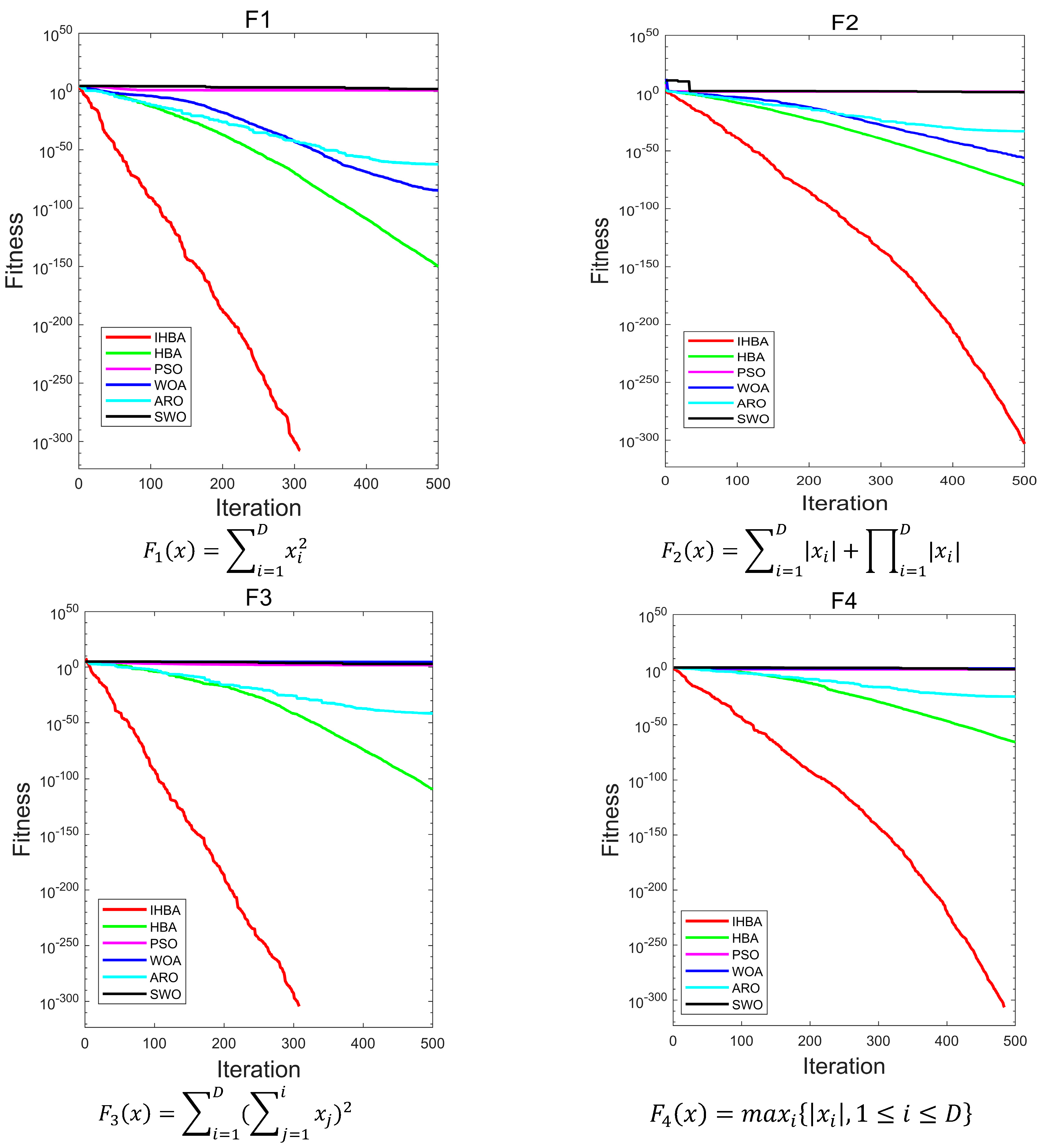
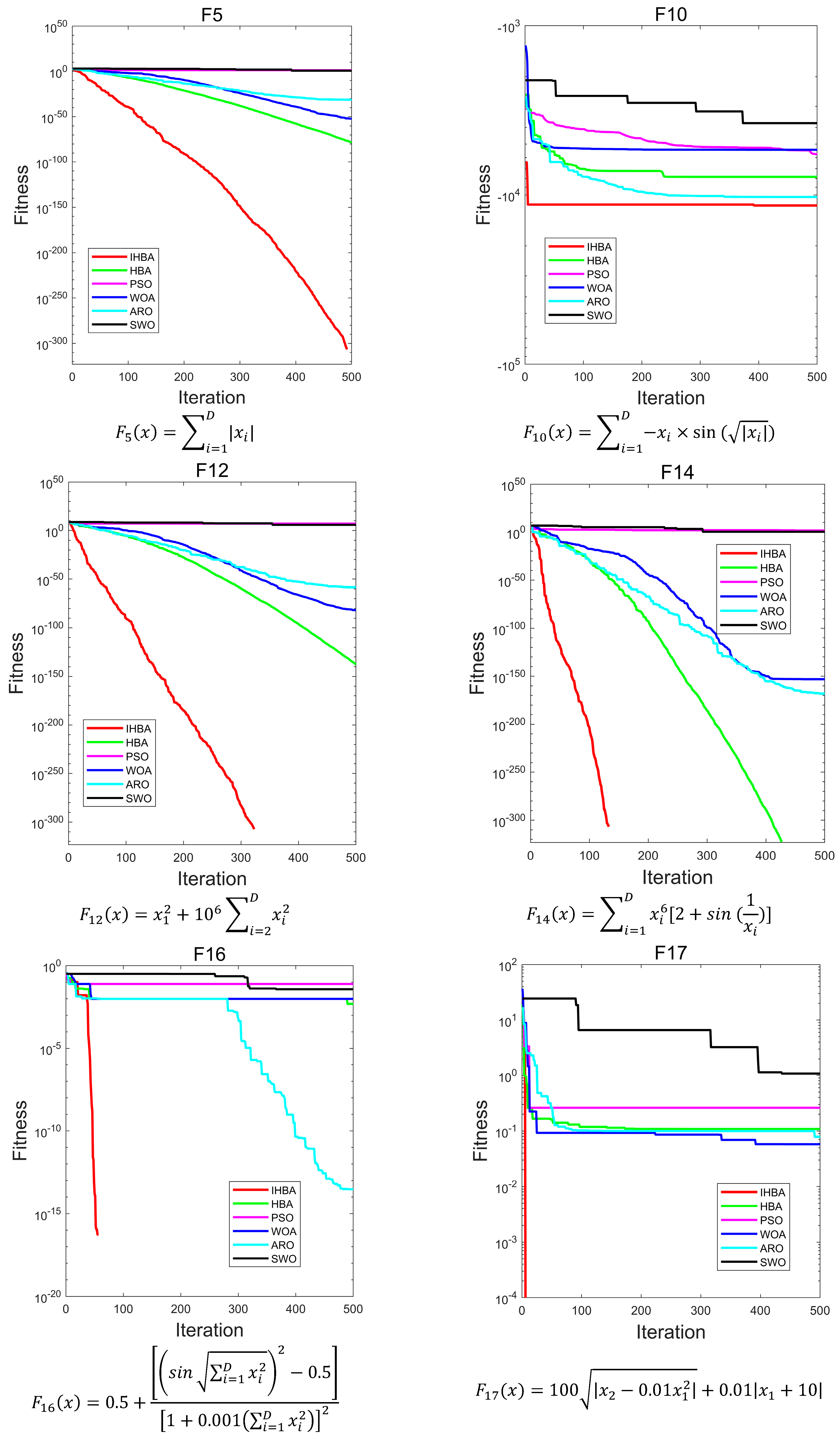
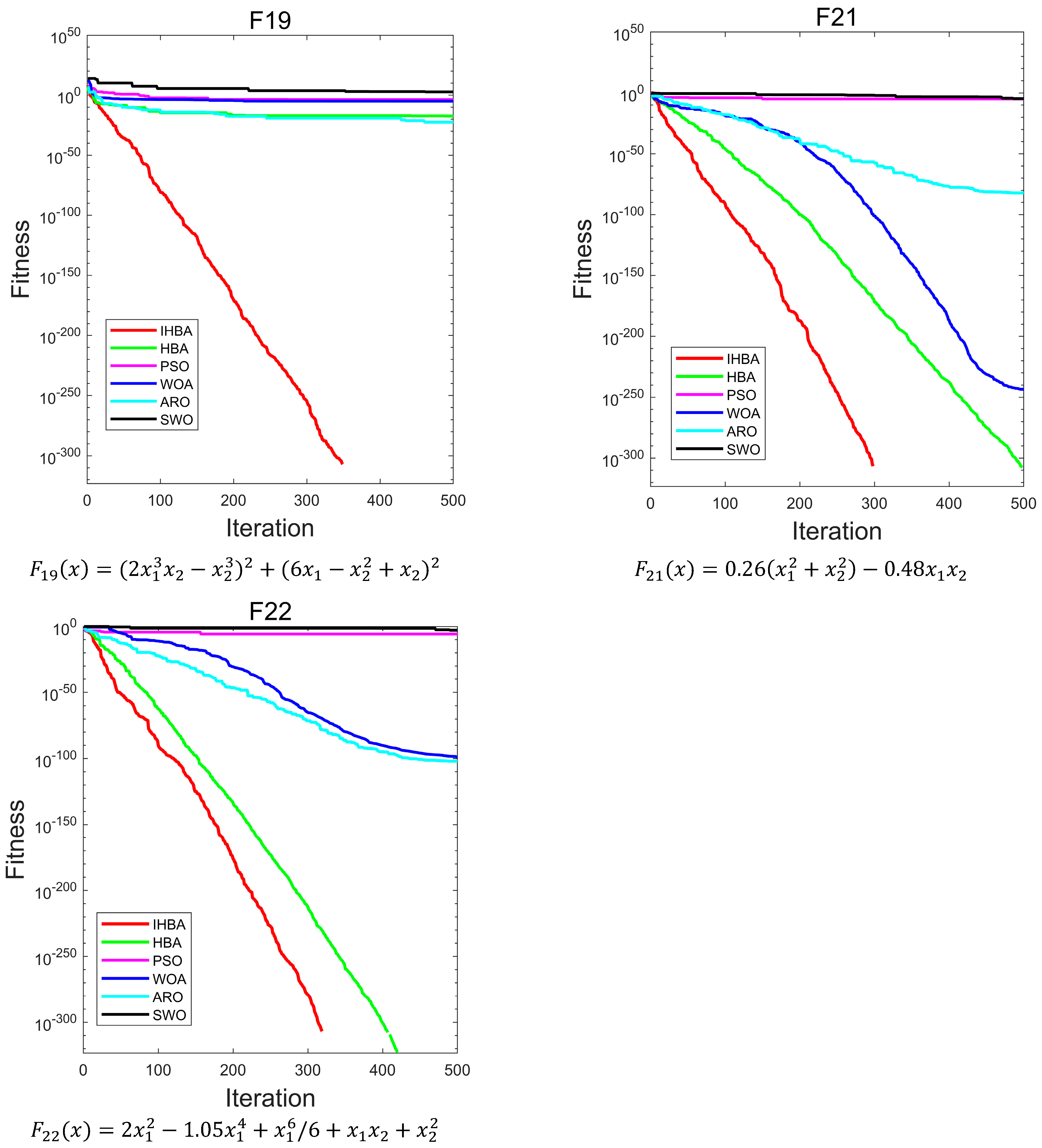
Figure 6 is a convergence diagram of the IHBA on the benchmark function. To ensure fairness, a population $N$ = 50, a maximum number of iterations $t_{max}$ = 500, and a dimension $D$ = 30 was set in the experiment. Each algorithm was run independently 30 times. Due to the limited space, this paper selected some test functions for convergence analysis and comparison. F1–F5 in single-peak test function; F10, F12, F14, and F16 in multi-peak test function; and F17, F19, F21, and F22 in constant-dimension test function were selected, respectively.

As illustrated in Figure 6, for the unimodal test functions, IHBA demonstrated the fastest convergence speed among the five algorithms. Additionally, IHBA achieved the highest search accuracy throughout the iterative process. In contrast, other algorithms converge slowly and have low convergence accuracy. In the multimodal test function, IHBA also converged quickly and achieved the highest search accuracy among the six algorithms, especially F14. Both IHBA and HBA found the optimal value of 0 in 500 iterations. However, by observing the convergence curve, IHBA converged more quickly than HBA, finding the optimal value first. This demonstrates the good performance of IHBA. In the fixed-dimension test function, IHBA performed well on F17, F19, F21, and F22. It was obviously better than the other comparison algorithms, and also performed well on F21. In general, IHBA showed a better performance.

5.3. Simulation Analysis of K-Means for Improved Honey Badger Algorithm

To further validate the practicality of IHBA, this study selected K-means, IHBA-KM, and K-means algorithm based on Honey Badger Algorithm (HBA-KM) for a clustering experiment comparison. This experiment selected three data sets from the UCI database. For details, see

Table 8. Data sets.

Data Sets	Iris	Wine	Glass
Class	3	3	6
Attributes	4	13	9
Sample size	150	178	214

.

In this paper, the error sum of squares (SSE), accuracy, and F-score were employed as metrics for evaluating clustering results.

SSE is a widely used metric for assessing the quality of clustering, referred to as fitness. It evaluates the sum of the squared distances between each data point and the center of its corresponding cluster. A lower fitness value signifies that a data point’s proximity to the clustering center correlates with improved clustering quality. The specific calculation formula is shown in Equation (16).

$$SSE={\sum }_{k=1}^k{\sum }_{x_i\in C_k}{\left|\right|x_i-u_k\left|\right|}^2$$

(16)

k denotes the number of clusters; $C_k$ represents all data points within the kth class; $x_i$ refers to the data points in the kth cluster; and $u_k$ signifies the center of that cluster.

Accuracy refers to the ratio of correctly clustered elements to the total number of elements, as expressed by the following equation. A higher accuracy indicates superior clustering results:

$$Accuracy={\displaystyle \frac{N_r}{N}}$$

(17)

$N_r$ represents the number of samples assigned to the correct cluster, and $N$ represents the number of samples.

The F-score is a widely used metric for evaluating clustering results, with a value range from 0 to 1. It reflects the degree of similarity between the clustering outcomes and the true classifications. A higher F-score, closer to 1, indicates a more effective clustering performance. Given the issue of class imbalance present in the data set utilized in this study, we employed the weighted F-score as a metric to evaluate the clustering outcomes. The specific formula is as follows.

$$\left\{\begin{array}{c}F-score=\left(1+{\beta }^2\right)\times {\displaystyle \frac{p\times r}{\left({\beta }^2\times p\right)+r}}\\ P={\displaystyle \frac{TP}{TP+FP}}\\ r={\displaystyle \frac{TP}{TP+FN}}\end{array}\right.$$

(18)

where TP is a true-false example, FP is a false-positive example, and FN is a negative-false example. $\beta =2$ when the data set is a class-unbalanced data set, which focuses more on small class recall, and $\beta =1$ when the data set is a class-balanced data set, which is the traditional F-score.

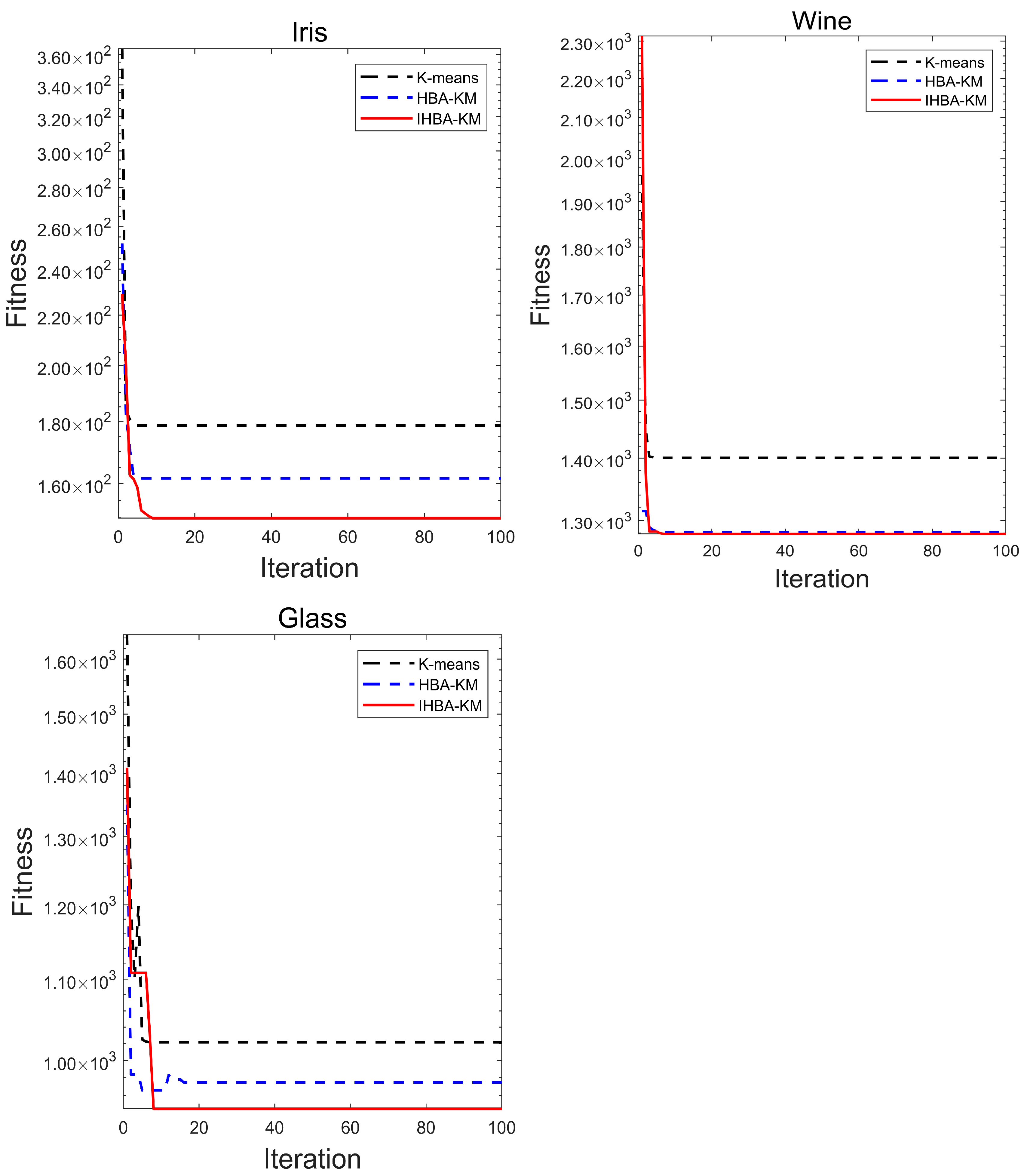
To ensure fairness, the parameters were kept consistent across all experiments: The number of populations was established at $N=20$, with a maximum iteration limit set to $t_{max}$ = 100. Each algorithm was executed independently a total of 30 times. The best, worst, and average values, along with the standard deviation, were recorded for each run. Experimental results are summarized in

Table 9. SSE comparison after running 30 times.

	Iris				Wine				Glass
Algorithms	Best	Worst	Mean	Std.	Best	Worst	Mean	Std.	Best	Worst	Mean	Std.
K-means	142.6	228.1	174.8	47.6	1287.0	1842.7	1045.4	43.9	837.0	1504.2	1105.0	114.2
HBA-KM	141.9	200.1	160.5	17.2	1278.5	1283.2	1279.5	1.3	810.1	1229.9	958.8	88.2
IHBA-KM	140.6	176.7	153.9	11.0	1278.4	1281.8	1278.9	0.74	810.6	1097.8	942.5	67.5

,

Table 10. Clustering accuracy comparison for 30 runs of each algorithm.

	Iris (%)			Wine (%)			Glass (%)
Algorithms	Mean	Best	Worst	Mean	Best	Worst	Mean	Best	Worst
K-means	80.73	85.33	66.66	87.68	93.82	59.55	56.65	59.34	48.13
HBA-KM	88.00	92.00	86.00	97.18	97.57	97.19	64.11	67.75	59.34
IHBA-KM	89.63	96.66	86.67	97.46	97.71	97.19	67.62	69.69	59.27

and

Table 11. F-score comparison for 30 runs of each algorithm.

	Iris			Wine			Glass
Algorithms	Mean	Best	Worst	Mean	Best	Worst	Mean	Best	Worst
K-means	0.73	0.76	65.05	0.81	0.88	0.61	0.40	0.50	0.32
HBA-KM	0.82	0.86	77.37	0.95	0.95	0.94	0.42	0.51	0.33
IHBA-KM	0.83	0.91	0.77	0.95	0.97	0.94	0.45	0.54	0.37

, while the convergence plots are shown in Figure 7.

Comparing the results of the K-means algorithm, HBA-KM, and IHBA-KM, the IHBA-KM algorithm showed obvious advantages in many indexes. According to Table 9, it can be seen that the IHBA-KM in Iris data set was much less adaptive; in terms of standard deviation, IHBA-KM was 54.87 higher than K-means and 6.6 higher than HBA-KM, which strongly proves that the clustering stability and quality of IHBA-KM algorithm are better. It is evident from Figure 7 that the three algorithms exhibited rapid declines during the initial stages of iteration. The K-means algorithm and HBA-KM finally fell into local optimal, while IHBA-KM emerged from the trap in search of a higher-quality solution. The findings illustrate the efficacy of IHBA-KM in clustering within the data set. Especially in the Glass data set, IHBA-KM had the smallest fitness value, and it was found through the convergence curve that the comparison algorithm fell into local optimal rapid convergence, while IHBA-KM jumped out of the trap of local optimal and obtained better clustering centers. However, the standard deviation of 67.5 also indicated that the stability of IHBA was poor, suggesting that the improvement measures in this paper can enhance the clustering effect, but there is still room for improvement.

In summary, IHBA-KM is superior to the traditional K-means algorithm and HBA-KM in terms of clustering effect, stability, and consistency. The experimental results show that the IHBA in this study can alleviate the influence of the initial clustering center on the clustering results and enhance the stability and efficiency of clustering.

In order to further evaluate IHBA-KM, this study continued to explore the use of the accuracy and F-score metrics as criteria. Detailed results can be found in Table 10 and Table 11.

The IHBA-KM showed significant advantages in multiple clustering tasks, especially in the accuracy index. Taking the Iris data set as an example, the average accuracy of IHBA-KM was 89.63%, higher than that of the K-means algorithm (80.73%) and HBA-KM (88.00%). In addition, the maximum accuracy of IHBA-KM was also outstanding, reaching 96.66%. The performance of this algorithm was markedly superior to those of other algorithms, suggesting that it possesses a greater capacity for achieving optimal clustering results. In the context of the Wine data set, IHBA-KM demonstrated a consistently high accuracy rate, averaging approximately 10% higher and achieving a minimum improvement of 27% compared to the K-means algorithm. This indicates its robustness and the stability in its performance. In the Glass data set, the average accuracy of IHBA was 67.62%, while the average accuracy of HBA stood at 64.11%. This represents an improvement of 3.51%, highlighting the positive impact of the enhanced strategy on classification performance. This stability and high accuracy make IHBA-KM a more reliable choice in practical applications, especially in scenarios where high-precision clustering results are required. On the whole, the IHBA-KM algorithm has obvious advantages in terms of clustering effect and accuracy.

As can be observed in Table 11, the IHBA-KM algorithm performed well on F-score indicators, especially on the Iris and Wine data sets. Its average F-score was 0.83, significantly higher than K-means’ 0.73 and HBA-KM’s 0.82. This enhancement reflects the effectiveness of IHBA-KM clustering. In terms of maximum F-score, IHBA-KM reached 0.91, surpassing the other two algorithms, indicating that it can achieve higher classification accuracy. In addition, its minimum F-score remained at 0.77, showing consistency and stability across different data sets. This advantage means that IHBA-KM can provide a reliable performance in a diverse array of application scenarios. In high-dimensional data, feature similarity often becomes less clear, negatively impacting clustering quality. Therefore, according to the Glass data set, the average F-scores for K-means and HBA were 0.40 and 0.42, respectively, while the average F-score for IHBA was 0.45. Compared to the other two algorithms, the clustering performance of IHBA on this data set was marginally superior; however, the relatively low values indicate a potential limitation of IHBA when applied to high-dimensional data.

In summary, the IHBA’s advantage in accuracy and F-score is unquestionable. By incorporating the HBA, IHBA reduces the reliance of the traditional K-means on the initial cluster centers. To address the issues of the HBA, including its vulnerability to local optima and slow convergence, the IHBA introduces several improvements. These enhancements help the algorithm to avoid local optima, speed up convergence, and ultimately enhance the overall efficacy of the clustering process.

6. Conclusions

In this study, an enhanced version of the HBA is proposed to address the issues of slow convergence and the tendency to become stuck in local optima. To improve the initial population distribution and the overall solution quality, chaos-based initialization was introduced at the beginning of the algorithm’s iterations. Additionally, the original density factor was modified to accelerate the algorithm’s convergence, further enhancing its performance. The nonlinear inertia weight was introduced into the formula of position updating to enhance the convergence rate of the algorithm. Random oppositional-based learning was implemented on the optimal individual to mitigate the risk of the algorithm converging to a local extremum. The IHBA was applied to K-means clustering to reduce the sensitivity of initial centroids. The results show that the IHBA-KM showed improved fitness, accuracy, and F1 indexes, and the clustering effect was better. However, the suboptimal performance of IHBA on the Glass data set underscores its limitations in high-dimensional clustering contexts. Future research will further explore enhancements to the Honey Badger Algorithm and the Sine Cosine Algorithm by integrating these approaches and will continue to explore the integration of alternative search strategies to improve their performance, aiming to continually improve algorithm performance. And furthermore, we aim to broaden its applicability in order to encompass multi-class clustering challenges, text clustering, feature selection, and other pertinent issues.

References

1. Djouzi, K.; Beghdad-Bey, K. A review of clustering algorithms for big data. In Proceedings of the 2019 International Conference on Networking and Advanced Systems (ICNAS), Annaba, Algeria, 26–27 June 2019; pp. 1–6. [Google Scholar]
2. Hu, H.; Liu, J.; Zhang, X.; Fang, M. An effective and adaptable K-means algorithm for big data cluster analysis. Pattern Recognit. 2023, 139, 109404. [Google Scholar] [CrossRef]
3. Sinaga, K.P.; Yang, M.-S. Unsupervised K-means clustering algorithm. IEEE Access 2020, 8, 80716–80727. [Google Scholar] [CrossRef]
4. Song, L.; Zhuo, Y.; Qian, X.; Li, H.; Chen, Y. GraphR: Accelerating graph processing using ReRAM. In Proceedings of the 2018 IEEE International Symposium on High Performance Computer Architecture (HPCA), Vienna, Austria, 24–28 February 2018; pp. 531–543. [Google Scholar]
5. Attari, M.Y.N.; Ejlaly, B.; Heidarpour, H.; Ala, A. Application of data mining techniques for the investigation of factors affecting transportation enterprises. IEEE Trans. Intell. Transp. Syst. 2021, 23, 9184–9199. [Google Scholar] [CrossRef]
6. Sun, Z.-H.; Zuo, T.-Y.; Liang, D.; Ming, X.; Chen, Z.; Qiu, S. GPHC: A heuristic clustering method to customer segmentation. Appl. Soft Comput. 2021, 111, 107677. [Google Scholar] [CrossRef]
7. Gong, R. Pattern Recognition of Control Chart Based on Fuzzy c-Means Clustering Algorithm. In Proceedings of the 2022 4th International Conference on Artificial Intelligence and Advanced Manufacturing (AIAM), Hamburg, Germany, 7–9 October 2022; pp. 899–903. [Google Scholar]
8. Ahmed, M.; Seraj, R.; Islam, S.M.S. The k-means algorithm: A comprehensive survey and performance evaluation. Electronics 2020, 9, 1295. [Google Scholar] [CrossRef]
9. Ikotun, A.M.; Ezugwu, A.E.; Abualigah, L.; Abuhaija, B.; Heming, J. K-means clustering algorithms: A comprehensive review, variants analysis, and advances in the era of big data. Inf. Sci. 2023, 622, 178–210. [Google Scholar] [CrossRef]
10. Das, P.; Das, D.K.; Dey, S. A modified Bee Colony Optimization (MBCO) and its hybridization with k-means for an application to data clustering. Appl. Soft Comput. 2018, 70, 590–603. [Google Scholar] [CrossRef]
11. Saremi, S.; Mirjalili, S.; Lewis, A. Grasshopper optimisation algorithm: Theory and application. Adv. Eng. Softw. 2017, 105, 30–47. [Google Scholar] [CrossRef]
12. Yang, X.-S.; He, X. Firefly algorithm: Recent advances and applications. Int. J. Swarm Intell. 2013, 1, 36–50. [Google Scholar] [CrossRef]
13. Yang, X.-S. Flower pollination algorithm for global optimization. In Proceedings of the International conference on Unconventional Computing and Natural Computation, Orléans, France, 3–7 September 2012; pp. 240–249. [Google Scholar]
14. Bai, L. K-means clustering algorithm based on improved quantum rotating gate artificial fish swarm algorithm and its application. Appl. Res. Comput. 2022, 39, 797–801. [Google Scholar]
15. Xie, H.; Zhang, L.; Lim, C.P.; Yu, Y.; Liu, C.; Liu, H.; Walters, J. Improving K-means clustering with enhanced Firefly Algorithms. Appl. Soft Comput. 2019, 84, 105763. [Google Scholar] [CrossRef]
16. Huang, P.; Luo, Q.; Wei, Y.; Zhou, Y. An equilibrium honey badger algorithm with differential evolution strategy for cluster analysis. J. Intell. Fuzzy Syst. 2023, 45, 5739–5763. [Google Scholar] [CrossRef]
17. Jiang, S.; Wang, M.; Guo, J.; Wang, M. K-means clustering algorithm based on improved flower pollination algorithm. J. Electron. Imaging 2023, 32, 032003. [Google Scholar] [CrossRef]
18. Li, Y.; Chu, X.; Tian, D.; Feng, J.; Mu, W. Customer segmentation using K-means clustering and the adaptive particle swarm optimization algorithm. Appl. Soft Comput. 2021, 113, 107924. [Google Scholar] [CrossRef]
19. Hashim, F.A.; Houssein, E.H.; Hussain, K.; Mabrouk, M.S.; Al-Atabany, W. Honey Badger Algorithm: New metaheuristic algorithm for solving optimization problems. Math. Comput. Simul. 2022, 192, 84–110. [Google Scholar] [CrossRef]
20. Han, E.; Ghadimi, N. Model identification of proton-exchange membrane fuel cells based on a hybrid convolutional neural network and extreme learning machine optimized by improved honey badger algorithm. Sustain. Energy Technol. Assess. 2022, 52, 102005. [Google Scholar] [CrossRef]
21. Chen, Y.; Feng, G.; Chen, H.; Gou, L.; He, W.; Meng, X. A multi-objective honey badger approach for energy efficiency enhancement of the hybrid pressure retarded osmosis and photovoltaic thermal system. J. Energy Storage 2023, 59, 106468. [Google Scholar] [CrossRef]
22. Arutchelvan, K.; Priya, R.S.; Bhuvaneswari, C. Honey Badger Algorithm Based Clustering with Routing Protocol for Wireless Sensor Networks. Intell. Autom. Soft Comput. 2023, 35, 3199–3212. [Google Scholar] [CrossRef]
23. Song, Y.; Lin, H.; Bian, Y. Improved DV_HOP Location Algorithm Based on distance Correction and Honey Badger Optimization. Electron. Meas. Technol. 2024, 45, 147–153. [Google Scholar]
24. Hu, G.; Zhong, J.; Wei, G. SaCHBA_PDN: Modified honey badger algorithm with multi-strategy for UAV path planning. Expert Syst. Appl. 2023, 223, 119941. [Google Scholar] [CrossRef]
25. Hussien, A.G.; Chhabra, A.; Hashim, F.A.; Pop, A. A novel hybrid Artificial Gorilla Troops Optimizer with Honey Badger Algorithm for solving cloud scheduling problem. Clust. Comput. 2024, 27, 13093–13128. [Google Scholar] [CrossRef]
26. Fathy, A.; Rezk, H.; Ferahtia, S.; Ghoniem, R.M.; Alkanhel, R. An efficient honey badger algorithm for scheduling the microgrid energy management. Energy Rep. 2023, 9, 2058–2074. [Google Scholar] [CrossRef]
27. Nassef, A.M.; Houssein, E.H.; Helmy, B.E.-d.; Rezk, H. Modified honey badger algorithm based global MPPT for triple-junction solar photovoltaic system under partial shading condition and global optimization. Energy 2022, 254, 124363. [Google Scholar] [CrossRef]
28. Yang, H.; E, J. Adaptive variable scale chaotic immune optimization Algorithm and its application. Control. Theory Appl. 2009, 26, 1069–1074. [Google Scholar]
29. Zhou, J.; Zhang, L.; Sun, T. Improved honey badger algorithm based on elite differential variation. Electron. Meas. Technol. 2024, 47, 79–85. [Google Scholar]
30. Arasomwan, M.A.; Adewumi, A. On the performance of linear decreasing inertia weight particle swarm optimization for global optimization. Sci. World J. 2013, 2013, 860289. [Google Scholar] [CrossRef]
31. WANG, T. Grasshopper optimization algorithm with nonlinear weight and Cauchy mutation. Microelectron. Comput. 2020, 37, 82–86. [Google Scholar]
32. Yuan, Y.; Mu, X.; Shao, X.; Ren, J.; Zhao, Y.; Wang, Z. Optimization of an auto drum fashioned brake using the elite opposition-based learning and chaotic k-best gravitational search strategy based grey wolf optimizer algorithm. Appl. Soft Comput. 2022, 123, 108947. [Google Scholar] [CrossRef]
33. Zhong, C.; Li, G.; Meng, Z.; He, W. Opposition-based learning equilibrium optimizer with Levy flight and evolutionary population dynamics for high-dimensional global optimization problems. Expert Syst. Appl. 2023, 215, 119303. [Google Scholar] [CrossRef]
34. Jiang, S.; Shang, J.; Guo, J.; Zhang, Y. Multi-strategy improved flamingo search algorithm for global optimization. Appl. Sci. 2023, 13, 5612. [Google Scholar] [CrossRef]
35. Feng, M.; Heffernan, N.; Koedinger, K. Addressing the assessment challenge with an online system that tutors as it assesses. User Model. User-Adapt. Interact. 2009, 19, 243–266. [Google Scholar] [CrossRef]
36. Kennedy, J.; Eberhart, R. Particle swarm optimization. In Proceedings of the ICNN’95-international conference on neural networks, Perth, WA, Australia, 27 November–1 December 1995; pp. 1942–1948. [Google Scholar]
37. Mirjalili, S.; Lewis, A. The whale optimization algorithm. Adv. Eng. Softw. 2016, 95, 51–67. [Google Scholar] [CrossRef]
38. Wang, L.; Cao, Q.; Zhang, Z.; Mirjalili, S.; Zhao, W. Artificial rabbits optimization: A new bio-inspired meta-heuristic algorithm for solving engineering optimization problems. Eng. Appl. Artif. Intell. 2022, 114, 105082. [Google Scholar] [CrossRef]
39. Abdel-Basset, M.; Mohamed, R.; Jameel, M.; Abouhawwash, M. Spider wasp optimizer: A novel meta-heuristic optimization algorithm. Artif. Intell. Rev. 2023, 56, 11675–11738. [Google Scholar] [CrossRef]
40. Jamil, M.; Yang, X.-S. A literature survey of benchmark functions for global optimisation problems. J. Math. Model. Numer. Optim. 2013, 4, 150–194. [Google Scholar] [CrossRef]
Figure 1. Inverse square law. I represents the intensity, S represents the prey position, and r is a random number that takes values from 0 to 1.
Applsci 15 00718 g001
Figure 2. Trajectories of honey badgers during the digging phase. Take the location of the prey as the origin.
Applsci 15 00718 g002
Figure 3. HBA flowchart.
Applsci 15 00718 g003
Figure 4. Comparison of original and improved density factors.
Applsci 15 00718 g004
Figure 5. IHBA flowchart. The blue squares represent the parts of the paper that have been improved.
Applsci 15 00718 g005
Figure 6. Convergence curves of each algorithm on different test functions.
Applsci 15 00718 g006aApplsci 15 00718 g006bApplsci 15 00718 g006c
Figure 7. Convergence curve of the algorithm on the data set.
Applsci 15 00718 g007