Tuning of a Viscous Inerter Damper: How to Achieve Resonant Damping Without a Damper Resonance

Abstract

Inerter dampers are effectively employed to mitigate and dampen structural vibrations in slender or high-rise buildings. The simple viscous inerter damper, with a viscous dashpot placed in series with an inerter, is designed to create resonant vibration damping, although the damper itself is without an internal resonance. The apparent resonant behavior is instead obtained by increasing the damper inertance until the two lowest modes of the considered building model interact, whereafter the viscous coefficient is adjusted until the desired response mitigation is achieved. The present modal interaction tuning requires that the reduced-order single-mode dynamic model of the building includes both inertia and flexibility from the (other) modes otherwise discarded by the model reduction. While the inertia correction adjusts the modal mass of the inerter damper, the corresponding flexibility introduces the apparent damper stiffness that creates the desired damper resonance. Thus, the accurate representation of other modes is essential for the design and resonant tuning of the simple viscous inerter damper. The resonant damper performance by the non-resonant viscous inerter damper is illustrated by a numerical example with a 20-story building model, for which the desired resonant modal interaction requires an inertance of almost ten times the entire translational building mass.

1. Introduction

In slender civil engineering structures, external dampers are used for response mitigation, the improvement of comfort, and earthquake protection (among others). The present paper proposes a simple viscous inerter damper, tuned to act resonantly for a building structure model, without an inherent damper resonance. Thus, the tuning of this apparent resonant damper is based on classic results for tuned mass dampers (TMDs), for which the book by Den Hartog [1] is considered a fundamental reference, introducing the so-called fixed-point tuning principle. For applications to civil engineering buildings, the fixed-point tuning principle results in different expressions for optimal stiffness and damping in the case of either harmonic steady-state response or white-noise stochastic excitation. An early and comprehensive summary of tuning expressions for various types of loading and response of a single-degree-of-freedom (sdof) structure model has been provided by [2], while the extension to full multi-dof (mdof) structures has mainly aimed at the numerical optimization of TMDs to narrow-band earthquake and/or wind loading [3]. In [4], the TMD is compared to a tuned liquid column damper (TLCD) for building vibrations, while recently, [5] considered the TMD inside Taipei 101 as a special case study. Recent review papers about the TMD damping of buildings structures are given in [6,7,8], emphasizing the wide application of TMDs for slender high-rise structures. For the present damper, optimal tuning is obtained by maximizing modal damping instead of mitigating response measures. For the TMD, this equal modal damping principle has been proposed in [9] and more recently extended to mdof structures in [10]. For the maximum damping approach, the tuning principle becomes independent of the particular loading and response type and thus results in a rather robust tuning principle.

1.1. Inerter Dampers

A recent extension of the classic TMD is the introduction of the so-called inverter, a two-terminal inertia element [11] that is most commonly realized by converting translational deflection into rotation [12], whereby gearing systems can be used to realize extraordinary large effective damper masses [13,14]. Because the absorber theory dictates that damper performance increases with damper mass, the mass gearing property has accelerated research and development of inerter-based devices.

The basic inerter-type dampers mostly combine the inerter with a spring and dashpot to create a fundamental resonant damper. The inerter and spring create a damper resonance that is commonly targeted to the dominant vibration mode of the structure. The fundamental analysis of tuned inerter dampers (TIDs) is introduced in [15], in which the damper is tuned to optimal response reduction, compared to the performance of the classic TMD, and investigated for mass ratios of up to 50% of the fundamental modal mass. In [16], tuning expressions for inerter dampers are carefully derived for various damper configurations and extended in [17] to maximize the base-isolation performance when the sdof structure is exposed to stochastic loading.

Analytical tuning expressions for TIDs are presented in [18,19], where the modal coupling with other modes is explicitly accounted for by additional (artificial) flexibility and inertia terms. This inclusion of residual mode correction enables the derivation of accurate explicit tuning formulae for inerter dampers, an approach also followed in the present paper. An exact numerical optimization of the two fundamental TIDs is conducted in [20,21] for an sdof structure exposed to stochastic base excitation.

Tuned inerter dampers have been proposed for several applications in high-rise building technology, such as for seismic retrofit [22,23] and the optimization of multiple TIDs for the vibration control of an mdof structure model under stochastic base excitation. Furthermore, inerter dampers have been extended by the introduction of negative-stiffness springs [24,25], which improves the TID’s damping capability, and by the installation of hysteretic dampers in [26].

A particular property of inerter elements is their theoretical ability to connect, and thus transfer force, between floors separated by several stories. An example is provided by [27], in which the inerter bridges four stories to create a larger relative damper deflection for the wind-induced vibration control of a high-rise building. The ultimate realization defines the so-called ground inerter damper, for which one of the inerter terminals is attached to the building support level. In [28], the inerter damper is tuned for optimal vibration damping, while in [29], the grounded concept is applied for seismic isolation.

The simplest case of grounded dampers are those acting as base-isolation systems. In [30], tuning expressions are derived optimal base-isolation applications of inerter dampers. As in [17], the optimally tuned inerter dampers aim at minimizing the transmissibility from base to structure. Inerter dampers are proposed for base-isolation of storage tanks by [31], while simple inerter systems (with hysteretic damping) are proposed for seismic isolation of building models in [32].

1.2. Hybrid Mass and Inerter Dampers

Because of the working similarity of TMDs and inerter-based TIDs, the merger of the two damper concepts has been considered extensively in the research literature, especially in connection with the damping and protection of building-type structures. The fundamental extension of the TMD by simply connecting an inerter between the auxiliary TMD mass and another building floor is introduced in [33] and referred to as the tuned mass damper inerter (TMDI). In [12], the TMDI is investigated in detail for various applications: vibration suppression, damper mass reduction, and the harvesting of energy. Subsequently, the TMDI has been considered in [34,35,36] for installation in building structures, focusing on harmonic excitation, earthquake loading, and wind-induced vibrations. As for the basic inerter dampers, the TMDI has been shown to possess superior base-isolation abilities with limited damper stroke in [37,38]. Furthermore, the TMDI also allows for the bridging of stories, as considered in [35,39] for wind-induced vibrations. In the detailed study in [39], it was shown that for a realistic bridging of stories, corresponding to the space occupied by a pendulum absorber, the classic TMD outperforms the TMDI.

More advanced inerter augmentations of the classic TMD have been proposed in the literature. The basic TMDI in [39] was improved by the extending the inerter by a spring and the TMD dashpot [14]. This more advanced TMD inerter device was shown in [14] to give better performance when tuned precisely. The inclusion of various inerter-type devices in the classic TMD is considered [16], whereby double-resonance absorbers are created. It is shown that these augmented absorbers create a very wide and flat plateau in the frequency response curves at the targeted structural frequency. Closed-form solutions for the tuning of such double-resonant TMD inerter absorbers were derived in [40] for the most common combinations of inerter, spring, and dashpot. Reviews of inerter-based dampers for structural vibration damping are given by [41,42].

1.3. Outline of Paper

The aim of the present paper is to design a simple viscous inerter damper, for which the inertance is chosen so that the first two structural vibration modes interact, creating an apparent resonant absorber characteristic, with a damper without an internal resonance. Section 2 introduces the mdof building model and the theory for attaching a general inerter damper. The system reduction from a full mdof model to a single-dof model for the targeted vibration mode includes the influence from the other modes by the residual stiffness and inertance terms, of the same form as in [18].

In Section 3, the viscous inerter damper is introduced, with a viscous dashpot placed in series with the inerter. This model is referred to as the C2 configuration in [17]. This viscous inerter damper is without a spring and thus is in itself non-resonant. However, because of the residual mode flexibility term, the characteristic equation for the reduced-order single-mode model is of quartic order in the complex natural frequency, whereby the equal modal damping from [9,18,43] can be applied to create resonant vibration damping. The residual mode correction coefficients are determined from the two limiting natural frequencies for vanishing (free) and infinite (clamped) viscous damper coefficients, following the general approach for vibration absorbers in [44]. However, in the present case, the damper is not resonant in itself, which is opposite to the absorbers in [44], which implies that the inertance of the present viscous inerter damper is calibrated by a simple iterative procedure to create the desired modal interaction between the first two modes of the building model. Section 3 concludes by tuning the viscous dashpot so that optimal frequency response curves are obtained for the response velocity amplitude of the structure.

The performance of the resonantly tuned viscous inerter damper is illustrated in Section 4 for the 20-floor building model in [14,39]. The damper is placed between ground and bottom floor, similar to a base-isolation system. The iterative tuning procedure gives a mass ratio of 10.5% of mode 1 modal mass, which is safely within what is considered applicable for inerter dampers in the literature. A root locus analysis, in which the complex-valued natural frequencies are traced in the complex plane for an increasing viscous coefficient, shows that the mass ratio tuning almost creates the desired bifurcation point condition. The subsequent frequency response analysis demonstrates that the novel resonant tuning of the simple viscous inerter damper creates a flat plateau for the top-floor velocity amplitude. The numerical example also investigates the influence of placing a spring in parallel to the dashpot, with a stiffness that is sufficiently small to not interfere too much with the sensitive resonant tuning but large enough to re-center the viscous inerter damper in practice (avoid drift).

The final conclusions in Section 5 highlight the conceptual novelty of the proposed damper configuration, which is simple and robust and creates the desired resonant type vibration mitigation, although the damper is without an internal resonance (no spring included).

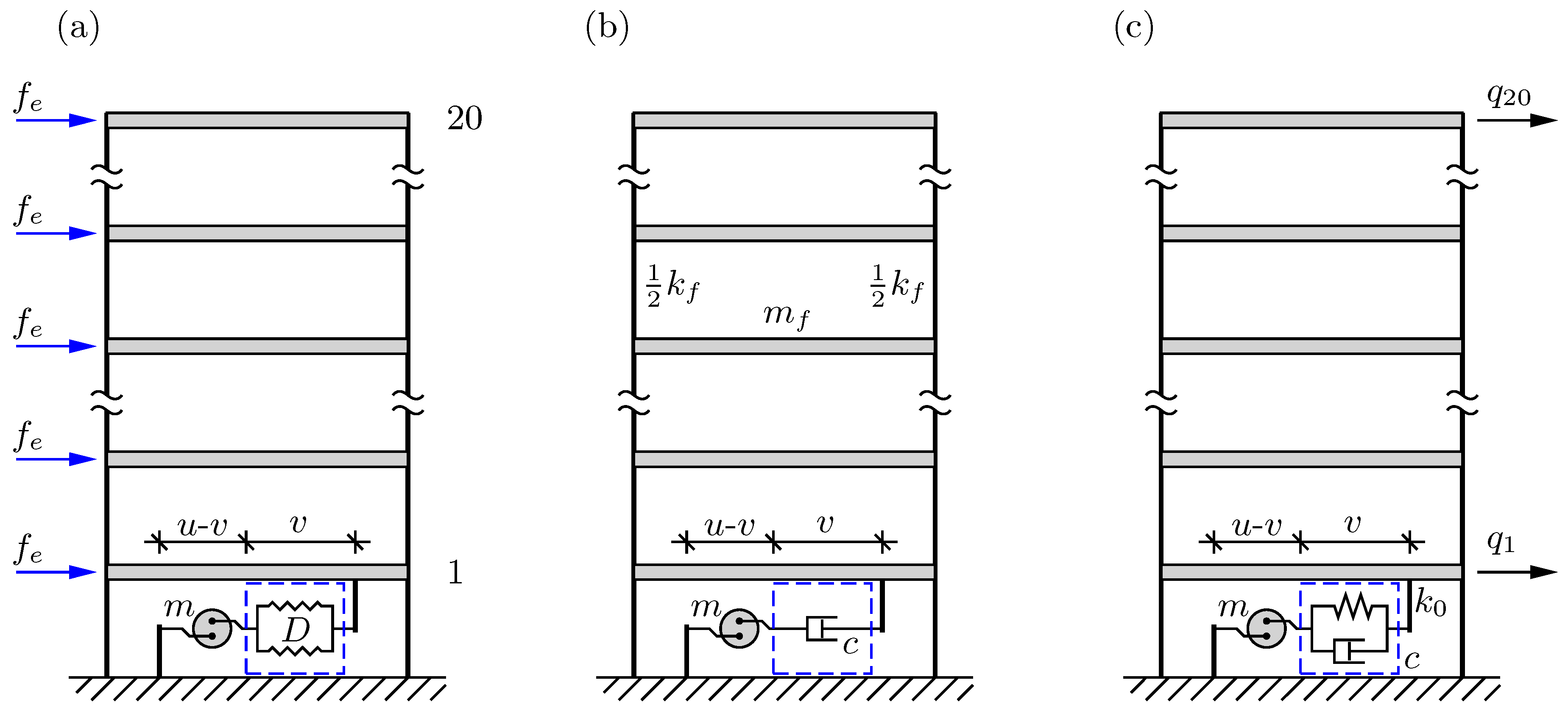
2. Governing Equations of Motion

Figure 1a shows a simple shear frame building model with $n=20$ stories. The story mass is assumed to be concentrated (lumped) at each floor, where it is denoted as $m_f$, while $k_f$ is the corresponding inter-story stiffness, as depicted in Figure 1b. The governing equation of motion in the time domain is then written in the common form as

$$\mathbf{M}\ddot{\mathbf{q}}\left(t\right)+\mathbf{C}\dot{\mathbf{q}}\left(t\right)+\mathbf{K}\mathbf{q}\left(t\right)+\mathbf{b}f\left(t\right)={\mathbf{f}}_{ext}\left(t\right)$$

(1)

where t is time and $\dot{\left(\right)}=d\left(\right)/dt$ represents the time derivative. For the present building model, the 20 floor displacements are collected in the displacement vector

$${\mathbf{q}}^T=[ q_1, q_2, \cdots , q_{20} ]$$

(2)

thereby constituting the governing degrees of freedom (dofs) for the present building model, which corresponds to the model used by Weber et al. [14,39]. In (1), $\mathbf{M}$ is the mass matrix, $\mathbf{C}$ is the damping matrix, and $\mathbf{K}$ is the stiffness matrix. The construction of the building model is presented in [14,39] and summarized in Section 4. The external loading is represented by the vector process ${\mathbf{f}}_{ext}\left(t\right)$, which in Figure 1a will be assumed to be evenly distributed across the building floors. Finally, $f\left(t\right)$ represents the force exerted by the inerter damper onto the structure, with the particular location of the damper determined by the connectivity vector $\mathbf{b}$. For the location between the ground and first floor in Figure 1, the connectivity vector is given as

$${\mathbf{b}}^T=[ 1, 0, \cdots , 0 ]$$

(3)

with entries 2 to 20 all zero.

Figure 1. Shear frame building model with an inerter damper (with inertance m) between the ground and the first floor. (a) General inerter damper with damper function $D\left(\omega \right)$, (b) viscous inerter damper with viscous coefficient c, and (c) viscoelastic inerter damper with viscous coefficient c and parallel spring stiffness $k_0$ introduced to avoid drift in dashpot deflection.

In the following damper design and tuning analysis, the behavior of the damper is conveniently represented in the frequency domain, in which time derivatives are included by 90-degree phase shifts. Thus, the time-based equation of motion (1) is conveniently converted into the frequency domain by introducing the steady-state frequency representations

$$\mathbf{q}\left(t\right)=\mathbf{q}exp\left(i\omega t\right),f\left(t\right)=fexp\left(i\omega t\right),{\mathbf{f}}_{ext}\left(t\right)={\mathbf{f}}_{ext}exp\left(i\omega t\right)$$

(4)

where the frequency variables $\mathbf{q}$, f, and ${\mathbf{f}}_{ext}$ represent steady-state amplitudes and thus are written without the time argument. By substitution of (4) into (1), the structural equation of motion can be expressed as a frequency relation in the following form

$$\left(-{\omega }^2\mathbf{M}+i\omega \mathbf{C}+\mathbf{K}\right)\mathbf{q}+\mathbf{b}f={\mathbf{f}}_{ext}$$

(5)

where the damper force f is defined in the following sections based on the inerter damper considered in the present paper. The frequency solution enables tuning based on both frequency response curves or pole-placement techniques. As shown for the classic tuned mass damper (TMD) in [9] and for general control methods in [43], a balanced pole-placement method will also provide effective response amplitude mitigation in frequency response curves. Thus, the pole-placement technique is applied in Section 3 for inerter damper tuning.

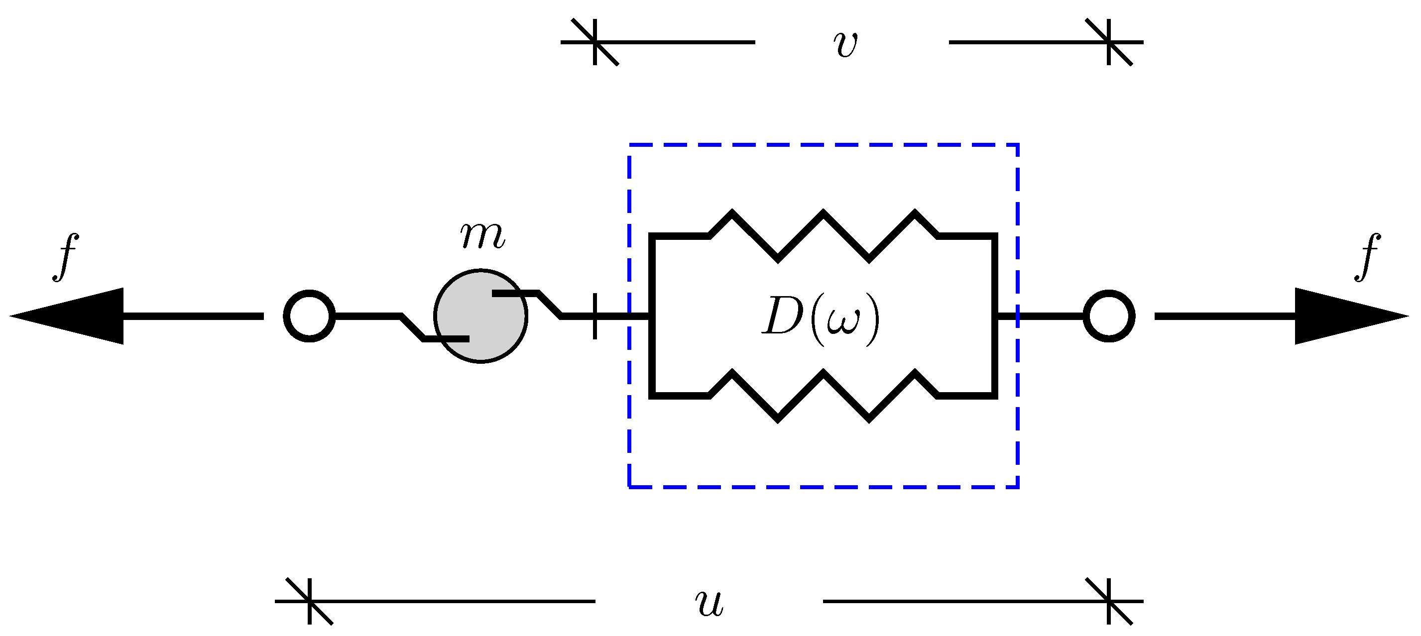
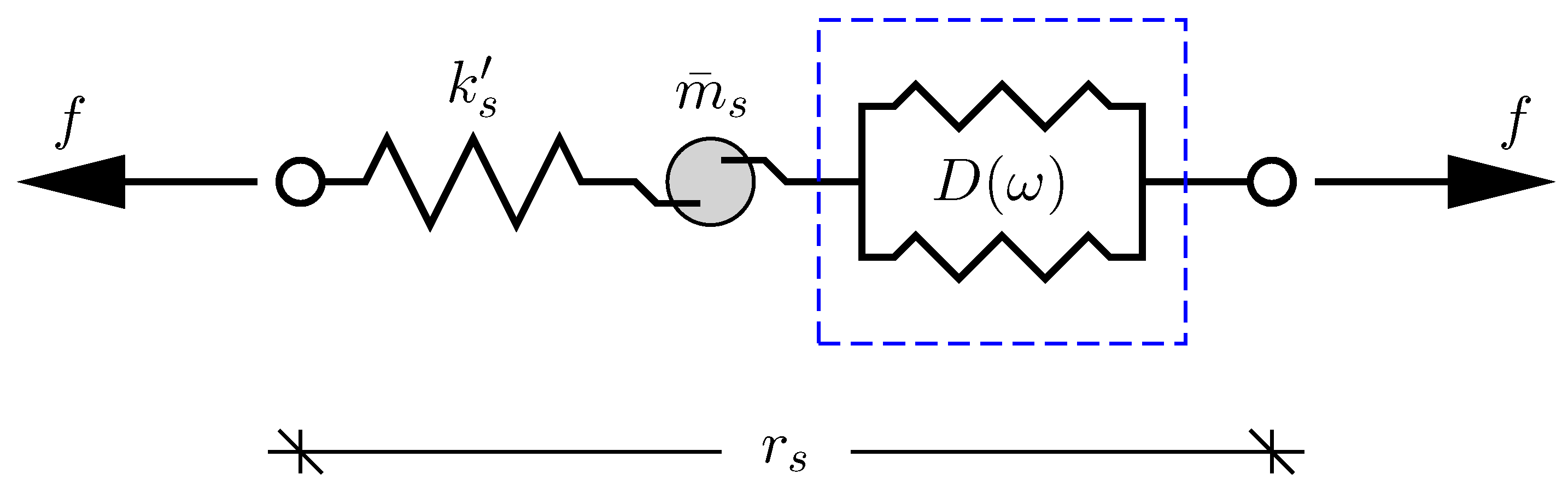
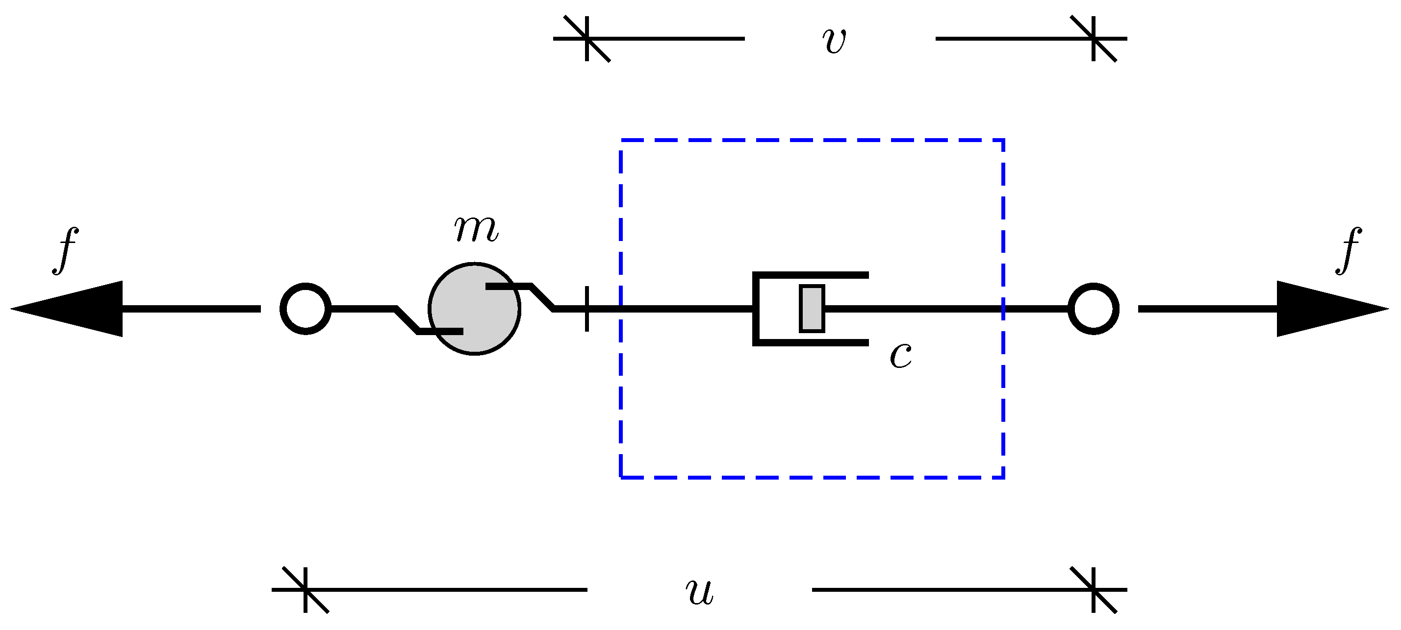
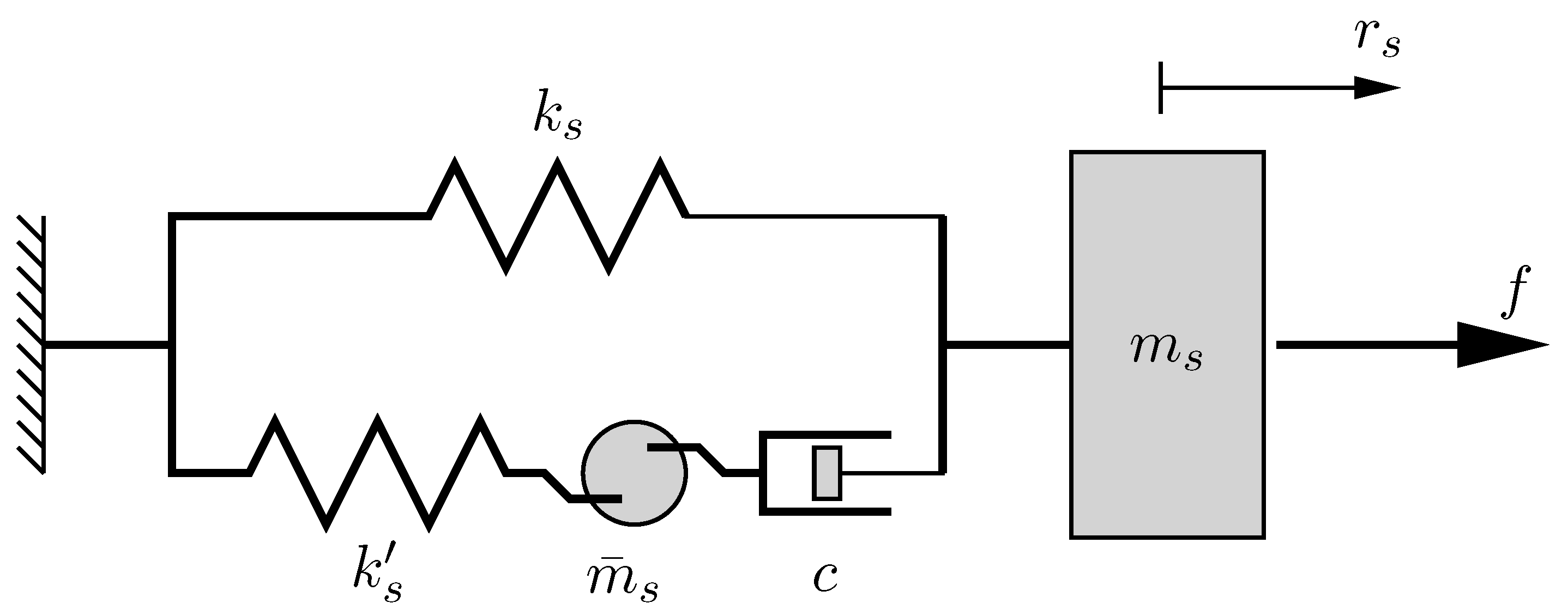
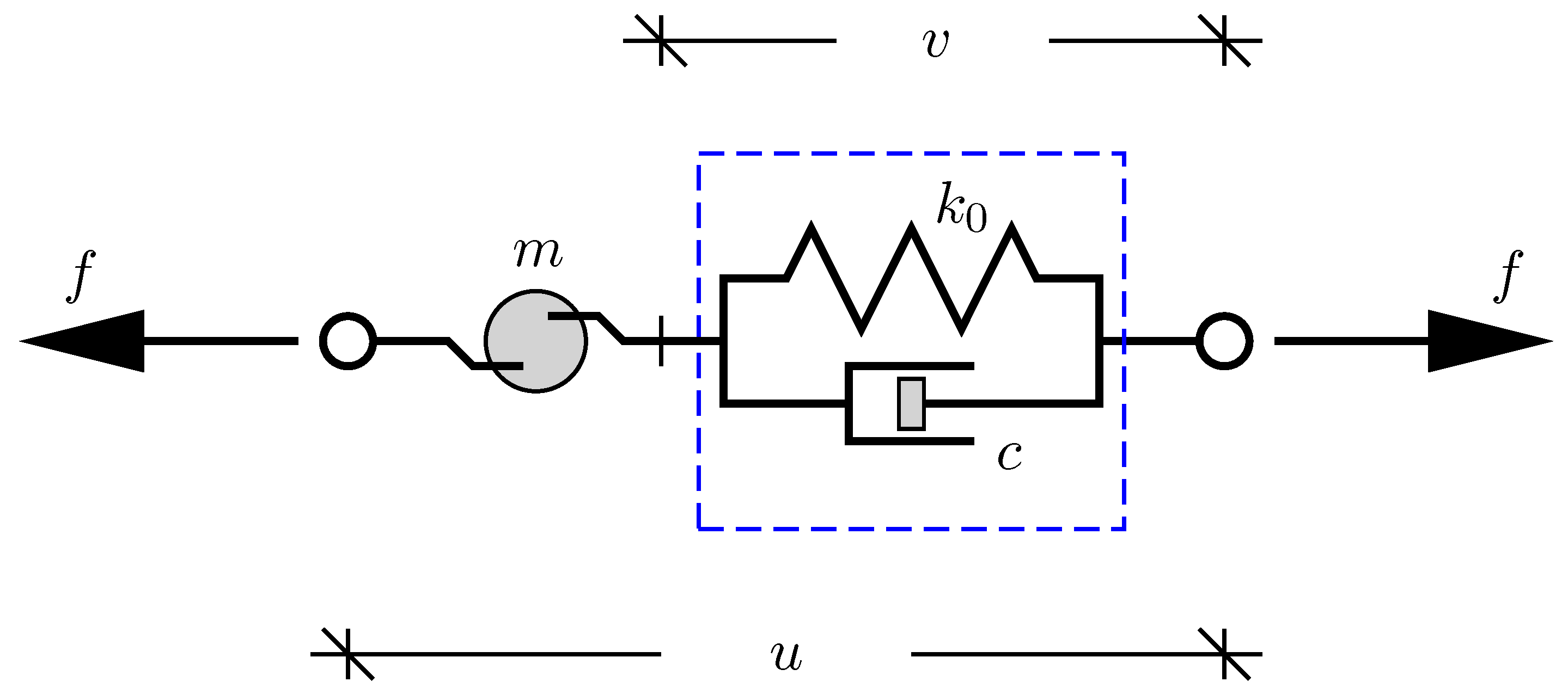
2.1. Inerter Damper Model

Inerter dampers can generally be constructed as an inerter (with inertance m) placed in series with an arbitrary damper element, which contains a viscous dashpot c in combination with springs and potentially additional inerters. This dynamic combination, placed in series with the front-end inerter m, is in the present (general) inerter damper model denoted $D\left(\omega \right)$; see Figure 2. This general inerter damper model is also used in Figure 1a when acting inside the building model. Furthermore, the figure shows two examples in (b) and (c), where the pure viscous inerter damper in Figure 1b is represented by $D\left(\omega \right)=i\omega c$, with c denoting the tunable viscous dashpot coefficient. In Figure 1c, the viscous dashpot is extended by a spring $k_0$ to (in principle) form a tuned inerter damper (TID) by the damper function $D\left(\omega \right)=i\omega c+k_0$. However, in the present case, the pure viscous damper function in Figure 1b is designed to operate resonantly by creating modal interaction between the two fundamental modes of the building structure, while $k_0$ in (c) is only introduced in the numerical example in Section 4 to avoid the drift of the damper stroke during operation.

Figure 2. General inerter damper with front-end inertance m in series with general damper element $D\left(\omega \right)$.

In the present section, the general inerter damper is assumed to be attached to the flexible dynamic structure, as shown for the building model in Figure 1a. The governing equation for the general inerter damper in Figure 2 is written in flexibility format as

$$\left({\displaystyle \frac{1}{-{\omega }^{2}m}}+{\displaystyle \frac{1}{D\left(\omega \right)}}\right)f=u$$

(6)

where the displacement u in Figure 2 represents the full stroke across the inerter damper. For the building model in Figure 1, this entire stroke u is determined by the connectivity vector as

$$u={\mathbf{b}}^T\mathbf{q}$$

(7)

which, therefore, by construction, is the energy conjugate displacement to the damper force f.

For the general inerter damper, the undamped case is retrieved by $D\to 0$, in which case $f=0$ in (6). On the other hand, for $D\to \infty$, the damper link, inside the blue-dashed box in Figure 2, will become fully rigid, thus ideally transferring the force, whereby $f=-{\omega }^{2}mu$ will add pure inertia to the structure. These two limiting cases will be important in the dynamic system reduction applied next.

2.2. Limiting Eigenvalue Problems

A typical damper design aims at optimizing the damping in a single vibration mode, which dominates the structural response of the structure. For high-rise buildings and other slender structures, such as wind turbines, towers, and masts, the dominant mode is likely the first (or fundamental) vibration mode. An effective system reduction procedure must isolate the targeted vibration mode, referred to below as mode number s, while still accounting for the spillover from all the other modes. For that, the present subsection introduces the limiting eigenvalue problems associated with $D\to 0$ and ∞, from which the corresponding natural frequencies are used to calibrate the modal spill-over to mode s from the non-targeted modes.

In Section 2.3, the modal expansion is based on the undamped vibration modes associated with $D=0$ and thereby $f=0$ from (6). In this free damper limit, the frequency equation of motion (5) simplifies to the generalized eigenvalue problem

$$\left(-{\omega }_j^2\mathbf{M}+\mathbf{K}\right){\mathbf{u}}_j=\mathbf{0}$$

(8)

for vanishing damping and external loading. In (8), the angular natural frequency ${\omega }_j$ is determined from the eigenvalue, while ${\mathbf{u}}_j$ is the associated mode shape vector for vibration mode j. Below, this undamped limit for $D\to 0$ is denoted as the free condition, whereby (8) is referred to as the free eigenvalue problem.

In the other limit $D\to \infty$—referred to below as the clamped limit—the damper element (inside the dashed-blue box) in Figure 2 will fully lock, whereby the generalized eigenvalue problem will change into

$$\left(-{\widehat{\omega }}_j^2(\mathbf{M}+m\mathbf{b}{\mathbf{b}}^T)+\mathbf{K}\right){\widehat{\mathbf{u}}}_j=\mathbf{0}$$

(9)

where m will increase the system’s inertia at the damper location. The hat symbol (^{^}) depicts solutions or parameters associated with the clamped limit, e.g., the clamped natural frequency ${\widehat{\omega }}_j$ and clamped mode shape vector ${\widehat{\mathbf{u}}}_j$. For the target mode $j=s$, it is assumed that the addition of inertia at the damper location will result in the clamped natural frequency being smaller than the associated free natural frequency, i.e., ${\widehat{\omega }}_s<{\omega }_s$.

In the next section, the free mode shapes are conveniently used in the modal expansion, as these mode shapes do not depend on the front-end inertance m of the inerter damper in Figure 2. Therefore, the clamped natural frequencies are used below to determine the influence from other modes, which in the present damper is of great importance, as the resonant damper characteristics are derived from modal interaction and not by an explicit damper resonant. The derivations are presented in the most compact form when both the free and clamped mode shapes are normalized to unit damper deflections, enforced by the relations

$${\mathbf{b}}^T{\mathbf{u}}_j=1,{\mathbf{b}}^T{\widehat{\mathbf{u}}}_j=1$$

(10)

For the indirect location of the inerter damper in Figure 1, the modal mass will be much larger than for a TMDI placed at the top floor, as in [14,39].

2.3. Modal Representation

As mentioned in the previous section, the free mode shapes are conveniently used in the modal expansion, as they are damper-independent because $D\to 0$ implies $f=0$. The modal representation of the structural displacement vector is therefore expressed as

$$\mathbf{q}=\sum _j{\mathbf{u}}_j{r}_j$$

(11)

The normalization in (10) to unit modal deflection across the inerter damper then simplifies the damper deflection u in (7),

$$u=\sum _j{\mathbf{b}}^T{\mathbf{u}}_j{r}_j=\sum _j{r}_j$$

(12)

which is simply the sum of modal coordinates. The governing (frequency-domain) modal equation of motion is obtained by substitution of (11) into (5), which, upon pre-multiplication by ${\mathbf{u}}_j^T$, can be written as

$$(-{\omega }^2{m}_j+k_j)r_j+f=f_j$$

(13)

This introduces the modal mass, stiffness, and load as

$$m_j={\mathbf{u}}_j^T\mathbf{M}{\mathbf{u}}_j,k_j={\mathbf{u}}_j^T\mathbf{M}{\mathbf{u}}_j,f_j={\mathbf{u}}_j^T{\mathbf{f}}_{ext}$$

(14)

while f appears un-scaled because of the unit-normalization of the free mode shape in (10).

In the free limit, where $f=0$ is realized by $D\to 0$ in (6), the solution to (13) must define the free natural frequency ${\omega }_j$ from the corresponding eigenvalue problem in (8). For $f_j=0$ and $f=0$, the modal equation of motion (13) determines the free natural frequency $\omega ={\omega }_j$ as

$${\omega }_j=\sqrt{{\displaystyle \frac{k_j}{m_j}} }$$

(15)

which corresponds to the well-known modal stiffness-to-mass ratio.

2.4. Residual Mode Correction

The damper force relation in (6) must be modified to give the damper force f as a function of (not u, but) the modal coordinate $r_s$ for the target mode s. This modal damper force relation will inherently contain spill-over from other modes ($j\ne s$), simply because the placement of a local damper, presently on the first floor, violates the modal orthogonality conditions. Substitution of the modal damper deflection representation (12) into the damper force relation (6) gives

$$\left({\displaystyle \frac{1}{-{\omega }^{2}m}}+{\displaystyle \frac{1}{D\left(\omega \right)}}\right)f=r_s+\sum _{j\ne s}{r}_j=r_s-\underset{1/R\left(\omega \right)}{\underbrace{{\sum }_{j\ne s}{\displaystyle \frac{1}{-{\omega }^2{m}_j+k_j}}}} f=r_s-{\displaystyle \frac{f}{R\left(\omega \right)}}$$

(16)

On the right-hand side of the first equality, the sum of $r_j$ is separated into $r_s$ for the target mode and a summation over all other (residual) modes $j\ne s$. The modal coordinates for these residual modes are replaced by the modal Equation (13) for $f_j=0$, which must be accurate for isolated tuning to mode $j=s$. Finally, in (16), all dynamic residual mode terms have f as a common factor, whereby they can be used in a general frequency-dependent residual mode function $R\left(\omega \right)$, to be determined below.

When collecting all terms proportional to the damper force f on the left-hand side, the inerter Equation (16) can be reduced to

$$\left({\displaystyle \frac{1}{-{\omega }^{2}m}}+{\displaystyle \frac{1}{D\left(\omega \right)}}+{\displaystyle \frac{1}{R\left(\omega \right)}}\right)f=r_s$$

(17)

which constitutes the governing damper equation for the target mode $j=s$. The closed-loop equations for mode s are thus composed of the modal Equation (13) for $j=s$ and the inerter damper force Equation (17).

As argued in [18,44,45,46], the influence from residual modes may be split into two separate components, representing stiffness and inertia. For the residual mode function $R\left(\omega \right)$ in (16), this separation can be expressed as

$${\displaystyle \frac{1}{R\left(\omega \right)}}\simeq {\displaystyle \frac{1}{-{\omega }^2{m}_s^{\prime }}}+{\displaystyle \frac{1}{k_s^{\prime }}}$$

(18)

with $m_s^{\prime }$ and $k_s^{\prime }$ representing artificial inertia and stiffness components that account for the interaction with other modes ($j\ne s$). For the present inerter damper, the substitution of this $1/R$ into the force relation (17) gives

$$\left({\displaystyle \frac{1}{-{\omega }^2{\overline{m}}_s}}+{\displaystyle \frac{1}{D\left(\omega \right)}}+{\displaystyle \frac{1}{k_s^{\prime }}}\right)f=r_s$$

(19)

which directly defines the combined inertance ${\overline{m}}_s$ by the reciprocal relation

$${\displaystyle \frac{1}{{\overline{m}}_s}}={\displaystyle \frac{1}{m}}+{\displaystyle \frac{1}{m_s^{\prime }}}$$

(20)

In the case of vanishing influence from residual modes, the reciprocal inertia correction will vanish ($1/m_s^{\prime }\to 0$), whereby the combined inertance recovers the front-end inertance, i.e., ${\overline{m}}_s\to m$. The modal damper model is shown in Figure 3, representing the modal damper relation (19) with combined inertance ${\overline{m}}_s$ and residual mode stiffness $k_s^{\prime }$. In the upcoming Section 3, these two system parameters are determined for a pure viscous inerter damper with a damper function $D=i\omega c$.

Figure 3. Model of mode s viscous inerter damper, with combined inertance ${\overline{m}}_s$ and additional spring stiffness $k_s^{\prime }$ to account for residual-mode flexibility.

For target mode $j=s$, the frequency response amplitude is conveniently derived from a frequency response function (FRF), which is obtained by eliminating f between (13) and (17). In normalized form, the FRF can then be expressed as

$${\displaystyle \frac{r_s{k}_s}{f_s}}={\displaystyle \frac{\left[-{\rho }^2{\overline{\mu }}_s+{\eta }_s\left(\rho \right)-{\rho }^2{\overline{\mu }}_s{\eta }_s\left(\rho \right)/{\kappa }_s^{\prime }\right]}{(-{\rho }^2+1)\left[-{\rho }^2{\overline{\mu }}_s+{\eta }_s\left(\rho \right)-{\rho }^2{\overline{\mu }}_s{\eta }_s\left(\rho \right)/{\kappa }_s^{\prime }\right]-{\rho }^2{\overline{\mu }}_s{\eta }_s\left(\rho \right)}}$$

(21)

when introducing

$$\rho ={\displaystyle \frac{\omega }{{\omega }_s}},{\overline{\mu }}_j={\displaystyle \frac{{\overline{m}}_j}{m_s}},\eta \left(\rho \right)={\displaystyle \frac{D\left(\omega \right)}{k_s}},{\kappa }_j^{\prime }={\displaystyle \frac{k_j^{\prime }}{k_s}}$$

(22)

as the frequency ratio ($\rho$), the effective mass ratio (${\overline{\mu }}_j$), the normalized damper function ($\eta$), and the stiffness correction ratio (${\kappa }_j^{\prime }$). The normalization of the combined mass ratio ${\overline{\mu }}_s$ in (22) implies that (20) can also be written in the non-dimensional form

$${\displaystyle \frac{1}{{\overline{\mu }}_s}}={\displaystyle \frac{1}{\mu }}+{\displaystyle \frac{1}{{\mu }_s^{\prime }}}$$

(23)

where the front-end and correction mass ratios

$$\mu ={\displaystyle \frac{m}{m_s}},{\mu }_j^{\prime }={\displaystyle \frac{m_j^{\prime }}{m_s}}$$

(24)

follow from the same definition as ${\overline{\mu }}_j$ in (22). The non-dimensional parameters and ratios defined in (22) and (24) are introduced in (21) and (23) for the target mode $j=s$.

3. Viscous Inerter Damper

The simplest damper function possible is the pure viscous dashpot, with

$$D\left(\omega \right)=i\omega c$$

(25)

in Figure 4. This simple series viscous inerter damper is shown attached to the present building model in Figure 1b, while in [16,17], it is referred to as a C2-type damper. By substitution of the viscous damper function in (25), the damper force relation (6) is given as

$$\left({\displaystyle \frac{1}{-{\omega }^{2}m}}+{\displaystyle \frac{1}{i\omega c}}\right)f=u$$

(26)

The present section will aim at a resonant design of this damper, where the extra resonance needed to create the resonance is not contained in the damper model, but instead obtained by controlled modal interaction between the two fundamental modes of the building structure.

Figure 4. Inerter damper with front-end inertance m in series with viscous dashpot, represented by the damper function $D\left(\omega \right)=i\omega c$.

3.1. Single-Mode Model

For the pure viscous inerter damper in Figure 4, the non-dimensional damper function $\eta$ in (22) can be expressed as

$$\eta ={\displaystyle \frac{i\omega c}{k_s}}=i\rho \beta$$

(27)

which introduces the non-dimensional damper ratio

$$\beta ={\displaystyle \frac{c}{\sqrt{k_s{m}_s }}}$$

(28)

Note that c is normalized by the modal mass and stiffness (and not the damper mass and stiffness). The damper function $\eta =i\rho \beta$ is then substituted into the modal frequency response function (21), which upon division of both numerator and denominator by $i\rho \beta$ can be written as

$${\displaystyle \frac{r_s{k}_s}{f_s}}={\displaystyle \frac{\left[i\rho {\displaystyle \frac{{\overline{\mu }}_s}{\beta }}+1-{\displaystyle \frac{{\rho }^2{\overline{\mu }}_s}{{\kappa }_s^{\prime }}}\right]}{(-{\rho }^2+1)\left[i\rho {\displaystyle \frac{{\overline{\mu }}_s}{\beta }}+1-{\displaystyle \frac{{\rho }^2{\overline{\mu }}_s}{{\kappa }_s^{\prime }}}\right]-{\rho }^2{\overline{\mu }}_s}}$$

(29)

with the damping parameter $\beta$ appearing in its reciprocal form. This FRF describes a single-dof structure model with modal coordinate $r_s$ and the augmented damper model in Figure 3 attached. This simplified structural model is shown in Figure 5, in which $m_s^{\prime }$ (contained in ${\overline{m}}_s$) and $k_s^{\prime }$ represent the interaction with the other modes ($j\ne s$). Thus, these correction parameters introduce the modifications needed to secure accurate modal results when reducing the system from the full mdof building mode in Figure 1b to the 2-dof (modal) model in Figure 5.

Figure 5. Resulting 2-dof model for mode $j=s$, combining the structural model with the modal coordinate $r_s$ and the viscous inerter damper with a combined inertance ${\overline{m}}_s$ and additional spring stiffness $k_s^{\prime }$ accounting for the interaction with residual modes ($j\ne s$).

The correction coefficients $m_s^{\prime }$ (or ${\overline{m}}_s$) and $k_s^{\prime }$ are determined in the next section so that the system poles (complex natural frequencies) approach the correct (real-valued) natural frequencies in the clamped limit. The characteristic equation, which governs the system poles, is identified from the denominator of the FRF in (21) as

$$(-{\rho }^2+1)\left(1-{\rho }^2{\displaystyle \frac{{\overline{\mu }}_s}{{\kappa }_s^{\prime }}}\right)-{\rho }^2{\overline{\mu }}_s+i\rho {\displaystyle \frac{{\overline{\mu }}_s}{\beta }} (-{\rho }^2+1)=0$$

(30)

It is worth noticing that finite values of ${\kappa }_s^{\prime }$ will imply that this equation has two complex conjugate solution pairs. For the viscous inerter damper with a small front-end inertance, the damper will act as a viscous damper, whereby the stiffness correction term must vanish for the characteristic equation to only have a single pair of complex conjugate poles. However, in the present design, the front-end inertance is increased until coupling with an adjacent vibration mode allows two system poles to interact and thereby create apparent resonant damper properties.

Figure 6 shows the trajectories of the complex system roots for the full 20-dof building model when attaching a pure viscous inerter damper. The equations of motion and the corresponding eigenvalue problem that governs the complex poles are presented in detail in Section 4. The blue circles “Fine with blue font” on the real frequency axis represent the free natural frequency ${\rho }_j={\omega }_j/{\omega }_1$. Thus, for mode $j=s=1$, the blue circle is by definition located at $\rho =1$ when $\eta =0$. On the other hand, the blue squares represent the clamped natural frequencies at $\rho ={\widehat{\omega }}_j/{\omega }_1={\widehat{\rho }}_j$, which the complex trajectories reach when $\eta \to \infty$.

Figure 6. Root loci for $\mu =0.067$ (a), 0.10 (b) and 0.15 (c). Free natural frequencies ${\omega }_j$ by circles and clamped natural frequencies ${\widehat{\omega }}_j$ by squares.

In the top subplot in Figure 6a, the front-end mass $m=0.067m_1$ chosen is slightly too small, as the damper trajectory approaches its clamped limit (blue square) at around $\rho \simeq 1.3$. For this inertance, the mode 1 locus is very small with limited attainable damping because of the very limited modal interaction between the mode 1 locus and the damper locus. In the next subplot (b), the front-end mass increases to $m=0.10m_1$, which clearly implies a great interaction with the mode 1 locus. It is seen that the two loci almost create a bifurcation point, which in the following is the tuning condition for the front-end inertance m. In the final subplot (c), the inertance is increased to $m=0.15m_1$, whereby the damper branch terminates at $\rho \simeq 0.75$, with little modal interaction and thus limited attainable damping for the semi-circular mode 1 locus. This sequence of plots in Figure 6 indicates that the optimal tuning must aim at creating a bifurcation point between the two clamped modes ${\widehat{\rho }}_1$ and ${\widehat{\rho }}_2$, with the free root at ${\rho }_1=1$ as the intermediate root that places a backbone curve that approaches the imaginary axis along the unit circle. Thus, the present damper shows that resonant damping, as tuned for a TMD or TID in [9,18], can be realized without having a stiffness–inertance damper element.

3.2. Correction Coefficients

For the damper ratio $\beta \to 0$, the solution to the characteristic Equation (30) becomes $\rho =0$ and $\rho =1$. In Figure 6, the undamped pole (or normalized free natural) frequencies are depicted by circles, which are located at the origin, at $\rho =1$ for mode 1 and then at $\rho ={\omega }_2/{\omega }_1\simeq 3$ for the next vibration mode $j=2$.

The aim of the tuning procedure is to place the first two clamped natural frequencies (${\widehat{\rho }}_1$ and ${\widehat{\rho }}_2$) so that they create apparent resonant absorber characteristics around the first free natural frequency $\rho =1$. Thus, the two solutions to the characteristic equation in (30) for $s=1$ must be

$${\widehat{\rho }}_1={\displaystyle \frac{{\widehat{\omega }}_1}{{\omega }_1}},{\widehat{\rho }}_2={\displaystyle \frac{{\widehat{\omega }}_2}{{\omega }_1}}$$

(31)

when $\beta \to \infty$.

In the clamped limit $\beta \to \infty$, the last term (proportional to $i\rho$) in (30) vanishes, whereby the characteristic equation reduces to

$${\rho }^4-{\rho }^2\left(1+{\kappa }_1^{\prime }+{\displaystyle \frac{{\kappa }_1^{\prime }}{{\overline{\mu }}_1}}\right)+{\displaystyle \frac{{\kappa }_1^{\prime }}{{\overline{\mu }}_1}}=0$$

(32)

with subscript $s=1$ indicating that the damper design targets the first vibration mode of the building model. For a given value of the front-end inertance m, the clamped natural frequencies are determined by solving the clamped eigenvalue problem (9). Thus, the solutions $\rho ={\widehat{\rho }}_1$ and ${\widehat{\rho }}_2$ to (32) are known from (9).

For the present normalization of the clamped-limit characteristic Equation (32), the product of the roots ${\widehat{\rho }}_1$ and ${\widehat{\rho }}_2$ is equal to the constant term, while the sum is the linear coefficient with the opposite sign. These relations can be used to solve for the modal damper parameters as a function of the clamped natural frequencies. The expressions can be written as

$${\overline{\mu }}_1=\left(1-{\displaystyle \frac{1}{{\widehat{\rho }}_2^2}}\right)\left({\displaystyle \frac{1}{{\widehat{\rho }}_1^2}}-1\right)$$

(33)

and

$${\kappa }_1^{\prime }=({\widehat{\rho }}_2^2-1)(1-{\widehat{\rho }}_1^2)$$

(34)

which are similar to the corresponding expressions for resonant inerter-based absorbers in [47]. When introducing ${\overline{\mu }}_1$ from (33), the correction mass ratio ${\mu }_1^{\prime }$ is isolated in (23) as

$${\displaystyle \frac{1}{{\mu }_1^{\prime }}}={\displaystyle \frac{1}{{\overline{\mu }}_1}}-{\displaystyle \frac{1}{\mu }}={\displaystyle \frac{1}{\left(1-{\displaystyle \frac{1}{{\widehat{\rho }}_2^2}}\right)\left({\displaystyle \frac{1}{{\widehat{\rho }}_1^2}}-1\right)}}-{\displaystyle \frac{1}{\mu }}$$

(35)

where the front-end mass ratio is $\mu =m/m_1$ is defined in (24).

3.3. Optimal Mass Ratio

As seen from the sequence of subplots in Figure 6, the optimal front-end inertance m is associated with the two branches meeting at a bifurcation point, similar to the tuning concept for a classic tuned mass or inerter damper [9,18]. This bifurcation point condition requires the two clamped roots $\rho ={\widehat{\rho }}_1$ and ${\widehat{\rho }}_2$ (squares) to be inverse points to the free root at $\rho =1$ (intermediate circle), which mathematically can be expressed by the simple relation

$${\widehat{\rho }}_1{\widehat{\rho }}_2=1$$

(36)

When this relation is squared, the product ${\widehat{\rho }}_1^2{\widehat{\rho }}_2^2$ is actually the product of the two roots to the clamped characteristic Equation (32), whereby ${\widehat{\rho }}_1^2{\widehat{\rho }}_2^2$ must equal the constant term in (32). This provides the optimality condition

$${\widehat{\rho }}_1^2{\widehat{\rho }}_2^2={\displaystyle \frac{{\kappa }_1^{\prime }}{{\overline{\mu }}_1}}=1\Rightarrow {\overline{\mu }}_1={\kappa }_1^{\prime }$$

(37)

which secures that the two complex roots meet at a bifurcation point.

The optimality criterion (37) is used to find the optimal front-end mass ratio $\mu$ by the relation

$${\displaystyle \frac{1}{\mu }}={\displaystyle \frac{1}{{\kappa }_1^{\prime }}}-{\displaystyle \frac{1}{{\mu }_1^{\prime }}}$$

(38)

where ${\overline{\mu }}_1$ has been eliminated by its definition in (23). If the residual mode ratios ${\kappa }_1^{\prime }$ and ${\mu }_1^{\prime }$ are determined with sufficient accuracy in (34) and (35), the expression (38) can be used directly to determine the front-end inertance m that secures optimal resonant damper behavior. However, in general, the inertance $m=\mu m_1$ from (38) will differ from the m used initially to solve the clamped eigenvalue problem in (9). Thus, the tuning of m is an inherently iterative process, conveniently solved by the stepwise procedure in Table 1.

Table 1. Tuning procedure for optimal front-end inertance m.

(1)	Choose m and determine $\mu =m/m_1$
(2)	Solve (9) and determined ${\widehat{\rho }}_1^2$ and ${\widehat{\rho }}_2^2$ from (31)
(3)	Determine ${\kappa }_1^{\prime }$ from (34) and ${\mu }_1^{\prime }$ from (35)
(4)	Update $\mu$ from (38) and $m=\mu m_1$
(5)	Repeat (2) to (4) until $\mu$ has converged

3.4. Optimal Damping

When the optimal front-end inertance is determined by the iterative procedure in Table 1, the optimal viscous coefficient c is chosen to optimize the attainable damping. In theory, the maximum damping is obtained exactly at the bifurcation point. However, as demonstrated in [9,18,43], the bifurcation point damper tuning results in interaction between the two modes associated with the first vibration form, which yields undesirable response amplification in FRF curves. Thus, for the present damper, the ratio ${\beta }_{bif}$ at the bifurcation point is multiplied by $\sqrt{2}$ to achieve a flat plateau in the frequency response curves. The FRF curves for optimal and bifurcation point damper ratios are compared in the numerical example in Section 4.5.

For the optimal mass ratio tuning ${\overline{\mu }}_1/{\kappa }_1^{\prime }=1$ in (37), the characteristic Equation (30) is readily reduced to

$${\rho }^4-{\rho }^2\left(2+{\overline{\mu }}_s\right)+1+i\rho {\displaystyle \frac{{\overline{\mu }}_s}{\beta }} (-{\rho }^2+1)=0$$

(39)

This characteristic equation secures that the two roots are inverse points to unity when $\beta \to \infty$, i.e., at the clamped damper limit. When reducing $\beta$, the complex poles move along semi-circular paths, still as inverse points to the unit circle. At the particular value $\beta ={\beta }_{bif}$, the two roots meet at a bifurcation point, after which they split and (approximately) trace the unit circle, with the pole approaching the real axis being the less damped and thus the pole governing the structural dynamics. When locating the poles with sufficient distance to the bifurcation point to avoid the dynamic interference between the two modes, the desired characteristic equation can be written as

$${\rho }^4-{\rho }^2\left(2+8{\zeta }_{\ast }^2\right)+1+i\rho \left(4{\zeta }_{\ast }\right)(-{\rho }^2+1)=0$$

(40)

as derived in [9,18,43]. In this equation, ${\zeta }_{\ast }$ represents the attainable damping ratio introduced by the inerter damper to the target mode, which in this case is the fundamental mode $s=1$.

The optimal $\beta ={\beta }_{opt}$ and the corresponding attainable damping ratio ${\zeta }_{\ast }$ are determined by one-to-one comparison between the actual characteristic Equation (39) for the present viscous inerter damper and the desired characteristic Equation (40). It follows directly from a comparison of the quadratic terms that the attainable damping ratio is

$${\zeta }_{\ast }=\sqrt{\frac{1}{8}{\overline{\mu }}_1}$$

(41)

which indicates that the damping ratio scales with the square root of the combined mass ratio ${\overline{\mu }}_1$, in practice evaluated by (33). Subsequently, the optimal damper ratio ${\beta }_{opt}$ is derived by comparison of the factors to the $(-{\rho }^2+1)$ parenthesis. This gives the optimal damper ratio

$${\beta }_{opt}=\sqrt{\frac{1}{2}{\overline{\mu }}_1}=2{\zeta }_{\ast }$$

(42)

as twice the attainable damping ratio. The tuning expressions (41) and (42) canonize the combined mass ratio ${\overline{\mu }}_1$ as the overall governing damper parameter that determines both tuning and performance.

4. Damping of the Building Model

The present section numerically investigates the proposed damper tuning, in which the viscous inerter damper is tuned to create modal coupling between the two fundamental modes of the 20 story model from [14,39], shown in Figure 1. In the equation of motion for the 20-floor model structure in [14,39], the mass matrix is diagonalized, while the stiffness matrix is a tri-band matrix based on assumed linear spring connections. Thus, the mass and stiffness matrix are composed as

$$\mathbf{M}=m_f\left[\begin{array}{cccc}1& & & \\ & 1& & \\ & & \ddots & \\ & & & 1\end{array}\right],\mathbf{K}=k_f\left[\begin{array}{cccc}2& -1& & \\ -1& 1& -1& \\ & -1& \ddots & -1\\ & & -1& 1\end{array}\right]$$

(43)

In the subsequent simulations, the structural damping matrix is omitted, whereby all damping is introduced by the viscous inerter damper.

4.1. Modal Parameters

The analytical expression for the natural frequency of this particular matrix structure can be derived from the finite difference discretization of a string [48], which gives

$${\omega }_j=2{\Omega }_{f}sin\left({\displaystyle \frac{\pi }{2}} {\displaystyle \frac{2j-1}{2n+1}}\right)$$

(44)

as shown in [49]. In this expression, the reference angular frequency ${\Omega }_f=\sqrt{k_f/m_f}$ is the natural frequency of a single-story building, i.e., for $n=1$. The floor mass is chosen as $m_f=5000 \mathrm{t}=5\times {10}^6 \mathrm{kg}$, whereafter the floor stiffness is determined from (44), which gives $k_f=659\times {10}^6$N/m when choosing ${\omega }_1/\left(2\pi \right)=0.14$Hz from [14,39]. The natural frequencies for the first 10 modes of the 20-dof building model are shown in the first row of Table 2. The second row presents the free modal mass for mode shapes normalized to unity deflection across the damper connection, i.e., $u_j=1$. For the present damper location, this means a unit first-floor deflection for each of the mode shapes. Therefore, the present modal masses are substantially larger than the common modal mass values obtained by normalizing the maximum mode shape deflection to unity. Furthermore, the modal mass decreases for increasing mode number, as the first floor deflection becomes relatively larger for higher mode shapes.

Table 2. Normalized natural frequencies and modal masses for free (top row) and clamped (bottom row) conditions. Frequencies are normalized by the free mode 1 natural frequency ${\omega }_1=2\pi \times 0.14 \mathrm{Hz}=0.88$rad/s, and modal masses are normalized by the free mode 1 modal mass $m_1=8746\times {10}^6$kg. The front-end inertance $m=919.4\times {10}^6$kg is obtained by the design procedure in Table 1.

j	1	2	3	4	5	6	7	8	9	10
${\rho }_j$	1.00	2.99	4.97	6.92	8.82	10.68	12.47	14.19	15.83	17.37
$m_j/m_1$	1.000	0.113	0.042	0.022	0.015	0.011	0.008	0.007	0.006	0.006
${\widehat{\rho }}_j$	0.853	1.17	3.16	5.23	7.27	9.26	11.2	13.1	14.8	16.5
${\widehat{m}}_j/m_1$	0.185	0.259	9.37	29.6	61.6	106.87	168.35	250.1	358.3	502.1

4.2. Tuning Parameters

The first overall task in the damper tuning is to determine the front-end damper inertance m using the iterative procedure in Table 1. In the present case, a first guess is chosen as $m=0.05m_1$, i.e., 5% mode 1 modal mass. The iterative procedure is run for 10 iterations, with a relative change of less than ${10}^{-12}$ for ${\overline{\mu }}_1=0.1051$ in the final iteration. The final inertance is then obtained as $m=919.4\times {10}^6$kg, which results in the governing tuning parameters in Table 3.

Table 3. Output from tuning procedure in Table 1.

$\mu$	${\overline{\mu }}_1$	${\mu }_1^{\prime }$	${\kappa }_1^{\prime }$	${\beta }_{opt}$
0.1051	0.1025	4.1440	0.1025	0.2264

For the optimal front-end inertance m, the clamped natural frequencies ${\widehat{\omega }}_j$ are obtained by solving the generalized eigenvalue problem (9). These frequencies are presented as ${\widehat{\rho }}_j={\widehat{\omega }}_j/{\omega }_1$ for target mode $s=1$ in the bottom half of Table 2. It is seen that ${\widehat{\rho }}_1{\widehat{\rho }}_2=1$, as required by the inverse point relation in (37a) and enforced by step (4) of the iterative tuning procedure in Table 1.

It is seen in Table 3 that the effective mass ratio ${\overline{\mu }}_1=0.1025$ is approximately equal to the actual mass ratio $\mu =0.1050$, which indicates that the correction by ${\mu }_1^{\prime }=4.1440$ in (23) is seemingly small. Thus, when using the common mass ratio in the damper tuning, i.e., ${\overline{\mu }}_1=\mu$, only moderate detuning is expected. In Table 3, the correction stiffness ratio ${\kappa }_1^{\prime }={\overline{\mu }}_1$, as required by (37), while the optimal damper ratio $\beta ={\beta }_{opt}$ from (42) secures a flat plateau in the frequency response curves. It is noted that the attainable damping is half of the damper ratio, which for the present case yields ${\zeta }_{\ast }=\frac{1}{2}\beta =0.113$ for damping of the first vibration mode ($s=1$).

4.3. Coupled Equations of Motion

As presented in Section 4.4 and Section 4.5, the damping and mitigation performance of the viscous inerter damper is assessed by root locus and frequency response analyses. For that purpose, the present section introduces the coupled equations for the damped structure in Figure 1. The equations also include the stiffness $k_0$ in Figure 7, which vanishes ($k_0=0$) in the ideal viscous inerter damper but is included in the numerical example to avoid drift between inerter and dashpot.

Figure 7. Inerter damper with front-end inertance m, in series with visco-elastic dashpot: $D\left(\omega \right)=k_0+i\omega c$.

A complex frequency—or pole—is derived from the damped eigenvalue problem, governed by the coupled Equations (5) for the structure and (26) for the viscous inerter damper. It is convenient to eliminate the force $f=-{\omega }^{2}y$, with $y=u-v$ being the deformation across the inerter. Thereby, the governing Equations (5) and (26) can be written in coupled form as

$$\left(-{\omega }^2\overline{\mathbf{M}}+i\omega \overline{\mathbf{C}}+\overline{\mathbf{K}}\right)\overline{\mathbf{q}}=\overline{\mathbf{f}}$$

(45)

introducing the augmented matrices

$$\overline{\mathbf{M}}=\left[\begin{array}{cc}\mathbf{M}& \mathbf{0}\\ {\mathbf{0}}^T& m\end{array}\right],\overline{\mathbf{C}}=\left[\begin{array}{cc}\mathbf{C}+c\mathbf{b}{\mathbf{b}}^T& -c\mathbf{b}\\ -c{\mathbf{b}}^T& c\end{array}\right],\overline{\mathbf{K}}=\left[\begin{array}{cc}\mathbf{K}+k_0\mathbf{b}{\mathbf{b}}^T& -k_0\mathbf{b}\\ -k_0{\mathbf{b}}^T& k_0\end{array}\right]$$

(46)

for the augmented displacement and load vector

$$\overline{\mathbf{q}}=\left[\begin{array}{c}\mathbf{q}\\ y\end{array}\right],\overline{\mathbf{f}}=\left[\begin{array}{c}{\mathbf{f}}_{ext}\\ 0\end{array}\right]$$

(47)

where the latter assumes that the inerter damper is unexposed to external forcing. These augmented matrices correspond to those derived for a classic TMD, with y representing the motion of the auxiliary TMD mass.

The complex system poles (or natural frequencies) are governed by the coupled equation of motion (45) without external loading ($\overline{\mathbf{f}}=\mathbf{0}$). This eigenvalue problem is conveniently solved in the first-order state space format

$$\left(\mathbf{A}-i\omega \mathbf{I}\right)\mathbf{z}=\mathbf{0}$$

(48)

where the system matrix and state-space vector are introduced as

$$\mathbf{A}=\left[\begin{array}{cc}\mathbf{0}& \mathbf{I}\\ -{\mathbf{M}}^{-1}\mathbf{K}& -{\mathbf{M}}^{-1}\mathbf{C}\end{array}\right],\mathbf{z}=\left[\begin{array}{c}\overline{\mathbf{q}}\\ i\omega \overline{\mathbf{q}}\end{array}\right]$$

(49)

It is noted that in (45) to (49), the entry $\mathbf{0}$ is the zero vector or matrix and $\mathbf{I}$ is the identity matrix that fit the given dimensions.

In Section 4.4, the first-order eigenvalue problem (48) is solved for a varying viscous coefficient c to trace the complex roots in a root locus diagram, as already applied in Figure 6. In Section 4.5, the frequency response curves are obtained by solving the frequency-domain equation of motion (45) for optimal tuning and varying (real-valued) angular frequency $\omega$. These analyses will illustrate the ability of the viscous inerter damper to realize apparent resonant damping, with $k_0$ being sufficiently small to not interfere while still large enough to avoid any drift across the viscous dashpot.

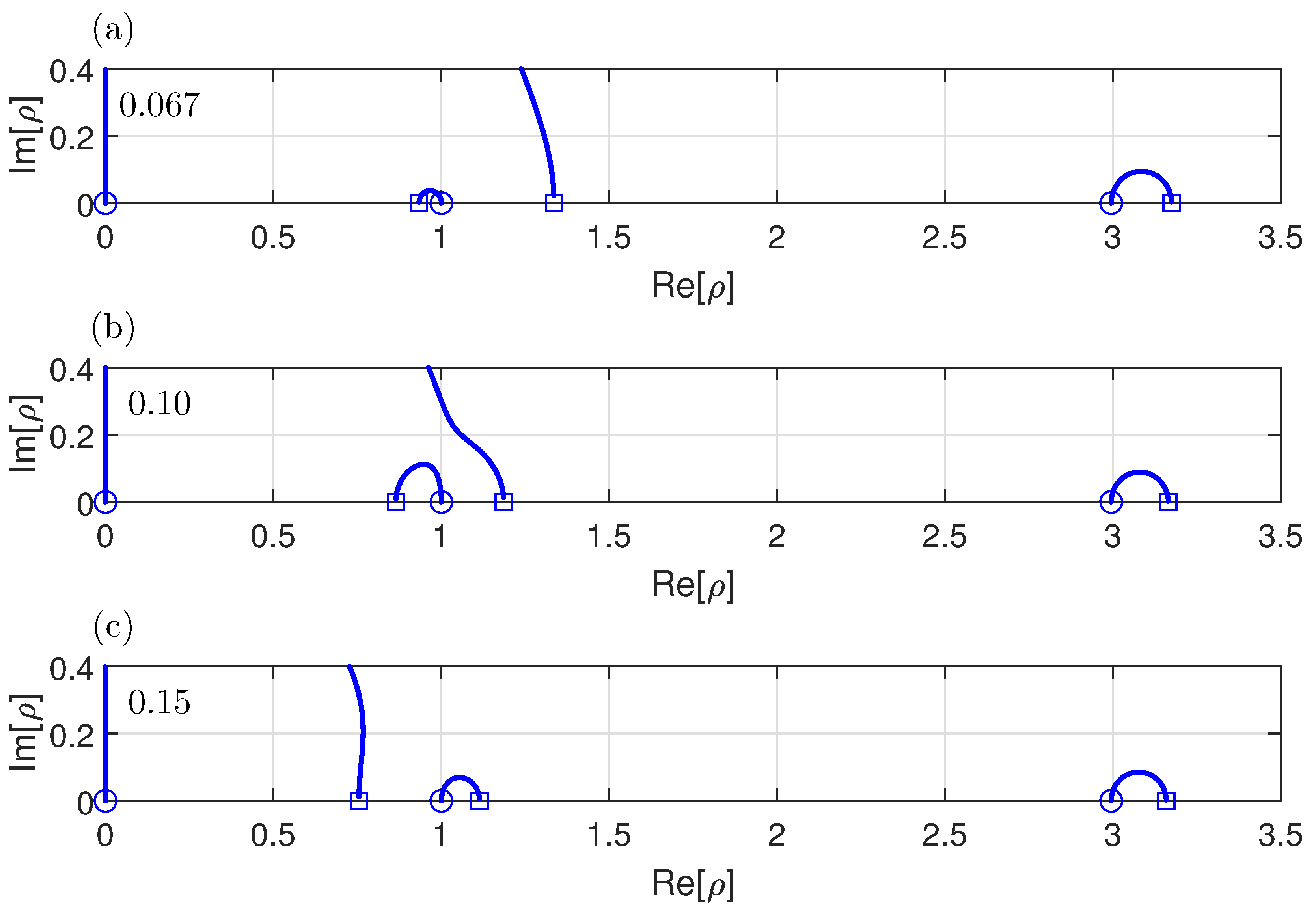
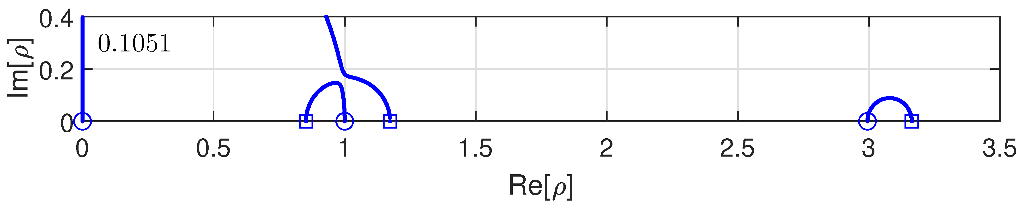
4.4. Root Locus Analysis

As shown by the sequence of root locus diagrams in Figure 6, the optimal tuning of the viscous inerter damper is derived from a modal interaction that creates a bifurcation point in the complex frequency plane (in this case the normalized $\rho$-plane). For the optimal front-end inertance, obtained by the design procedure in Table 1 and summarized in Table 3, the complex poles $\rho =\omega /{\omega }_1$ are obtained by solving the eigenvalue problem (48) from $c\to 0$ to $c\to \infty$. Figure 8 shows the root locus diagram for the optimally tuned viscous inerter damper. By comparison with the almost optimal loci in Figure 6b for $\mu =0.1000$, the optimal tuning curve in Figure 8 for $\mu =0.1051$ almost realizes the desired bifurcation point. The circles represent the free natural frequencies, while the squares are the clamped natural frequencies. The tuning procedure in Table 1 secures that the product of the first two normalized roots is unity, according to the inverse point relation in (37).

Figure 8. Root loci for inertance tuning to mode $s=1$. The front-end mass ratio $\mu =0.1051$ is obtained by the tuning procedure in Table 1.

Figure 9a shows a detailed plot of the semi-circular loci for the mode 1 roots. The circle represents the real-valued root for $\beta \to 0$. The other free limit root is located at the origin, as depicted by the circle at the origin in Figure 8. For increasing $\beta$, the root from $\rho =1$ moves into the complex plane, approximately along the backbone unit circle, toward the bifurcation point. The other root leaves the origin along the imaginary axis, meets its conjugate pole decending from $\rho =i\infty$, whereby it follows the backbone unit circle toward the bifurcation point. In the present case, the root from $\rho =1$ branches off before the ideal bifurcation point and traces the semi-circular path towards the smaller of the two clamped natural frequencies (blue square), while oppositely, the root from the imaginary axis follows the semi-circular path toward the larger clamped frequency.

Figure 9. (a) Root loci for mode 1 with asterisk (∗) depicting the roots for the optimal $\beta ={\beta }_{opt}$ by (42). (b) Ideal root locus diagram from the quartic polynomial in (39).

The ideal root locus diagram is obtained by solving the quartic polynomial in (39) with optimal ${\overline{\mu }}_1$ and plotted in Figure 9b. It is seen that for the idealized sdof model, without actual influence from other modes, the two semi-circular branches do meet exactly at a bifurcation point, where the damper parameter is ${\beta }_{bif}={\beta }_{opt}/\sqrt{2}=\sqrt{\frac{1}{4}{\overline{\mu }}_1}$. Thus, the inability of the root loci for the 20-story shearframe building model in Figure 9b to exactly meet at a bifurcation point indicates the approximations applied in the representation of residual mode effects in Section 3.2.

In the root locus diagram in Figure 9, the asterisks represent the roots for optimal $\beta$ from the design formula (42). The inclined straight line intersects the origin, whereby its inclination approximates the modal damping ratio. It is seen that both optimal roots are placed on the same line, which demonstrates a balanced damper design, where both roots associated with the target mode 1 are equally damped. The two damping ratios ${\zeta }_{1-}$ and ${\zeta }_{1+}$ at the two asterisks in Figure 9 are presented in Table 4 for $k_0=0$. It is seen that the two damping ratios for mode 1 and $k_0=0$ are identical ($0.1126$) to the fourth decimal and practically equal to ${\zeta }_{\ast }=0.1132$, which validates the accuracy of the proposed inertance tuning procedure in Table 1.

Table 4. Damping ratios ${\zeta }_{1-}$ and ${\zeta }_{1+}$ for the two mode 1 poles for optimal tuning from Table 3. Prediction of maximum attainable damping: ${\zeta }_{\ast }=\frac{1}{2}{\beta }_{opt}=0.1132$.

$\mu$	$k_0=0$	$k_0=0.05 {\omega }_1^{2}m$	$k_0=0.1 {\omega }_1^{2}m$
${\zeta }_{1-}$	0.1126	0.1159	0.1190
${\zeta }_{1+}$	0.1126	0.1106	0.1084

As indicated in Figure 1c, the pure viscous inerter damper is in practice implemented with a spring in parallel to the dashpot to avoid drift in the damper stroke. It is important to note that in the present analysis, the stiffness $k_0$ of the spring is not chosen to create an additional resonance with the front-end inertance m and thus kept sufficiently small to avoid dynamic interaction with mode 1. As indicated in Table 4, the spring stiffness $k_0$ is chosen as 0%, 5%, and 10% of the stiffness needed for the isolated damper frequency ${\omega }_0=\sqrt{k_0/m}$ to equal the free mode 1 frequency ${\omega }_1$. Figure 10 shows the root loci for mode 1 for the three different choices of damper stiffness: $k_0=0$ (blue), $k_0=0.05 {\omega }_1^{2}m$ (magenta) and $k_0=0.1 {\omega }_1^{2}m$ (red). Thus, the blue trajectories are identical to those in Figure 9. For finite values of $k_0$, the damper locus initiates from a small real-valued root (magenta and red circles) and not the origin (blue circle). For increasing values of $\beta$ and sufficiently small values of $k_0$, the damper root approaches the imaginary axis and follows a path that is qualitatively similar to that explained for the pure viscous inerter damper in Figure 9. It is seen from the local mode 1 trajectories that increasing $k_0$ implies a slight (and further) deterioration of the bifurcation point property. To assess the reduction in attainable damping, the two damping ratios for optimal $\beta$ are also presented in Table 4. It is seen that the damping ratio ${\zeta }_{1-}$ for the lower frequency branch increases with $k_0$, while conversely, the higher-branch damping ratio ${\zeta }_{1+}$ is reduced. Thus, the attainable damping (in this case the smaller ${\zeta }_{1+}$) is reduced by 2% and 4% compared with the equal damping ratios for the pure viscous inerter damper (for $k_0=0$). Thus, including the low-stiffness spring $k_0$ has a limited effect on the overall damper performance, while it secures the mechanical centering of the damper during operation. In practice, it is therefore recommended to install a $k_0$-spring in parallel with the dashpot, which by itself would create a damper resonance (with m) a decade below the targeted natural frequency.

Figure 10. Root loci for mode 1 for $k_0=0$ (blue), $k_0=0.05 {\omega }_1^{2}m$ (magenta) and $k_0=0.1 {\omega }_1^{2}m$ (red).

4.5. Frequency Response Analysis

The present resonant tuning of the viscous inerter damper hinges on the creation of a bifurcation point in the complex root diagram; see Figure 8, Figure 9 and Figure 10 in the previous section. Thus, the initial validation in Section 4.4 investigates the root loci for the target mode 1 for the pure viscous inerter damper ($k_0=0$) and for sufficiently small values of the restoring spring’s stiffness $k_0$. However, in structural dynamics, the tuning of resonant dampers is most commonly assessed by the reduction in frequency amplitudes, i.e., by the inspection of the frequency response curves (or FRFs).

The ideal frequency response curves for the present resonant damping device are obtained from the sdof FRF in (21), in which the optimal damper ratio $\beta ={\beta }_{opt}$ is contained in $\eta =i\rho \beta$. These sdof FRF curves are shown in Figure 11. From the frequency displacement curve in Figure 11a it is seen that the equal damping calibration used in Section 3.3 to determine the optimal mass ratio will not provide a flat plateau in the FRF for the displacement variable. Instead, the curve is slightly inclined, with a larger low-frequency peak. However, the equal damping calibration yields a flat plateau for the structure velocity amplitude in Figure 11a. Although not shown, the acceleration amplitude will then have an opposite inclination to that for the displacement in (a), whereby the present tuning (with a flat velocity amplitude curve) might be a decent compromise between minimizing displacement to optimize load-carrying capacity and minimizing acceleration to optimize comfort.

Figure 11. Frequency response functions for idealized sdof model from (21): (a) modal displacement amplitude and (b) modal velocity amplitude.

Figure 12 shows the frequency response curves for the full 20-story building model with the viscous inerter damper placed between the ground and first floor, as shown in Figure 1. The curves are obtained by solving the frequency equation of motion in (45) with evenly distributed forcing by

$${\mathbf{f}}_{ext}=f_{ext}{[ 1, 1,\cdots , 1 ]}^T$$

where the scalar $f_{ext}$ denotes the loading intensity. Since the response curves in Figure 12 are normalized by the corresponding static deflection ${\mathbf{q}}_0={\mathbf{K}}^{-1}{\mathbf{f}}_{ext}$, the actual value of $f_{ext}$ is irrelevant in the present linear analysis.

Figure 12. Frequency response functions for mode 1: (a,b) Top-floor motion $q_{top}$, (c,d) damper motion v, (a,c) displacement amplitude, and (b,d) velocity amplitude.

Figure 12a shows the top floor displacement amplitude, while (b) shows the corresponding velocity amplitude. The two bottom subfigures (c) and (d) show the displacement and velocity amplitudes for the damper stroke $v=u-y$ across the damper dashpot. The blue curves are for vanishing damper stiffness ($k_0=0$), while the red curves represent $k_0=0.1 {\omega }_1^{2}m$ (red), as in the previous root locus diagrams. The solid-line curves represent the optimal damper parameter $\beta ={\beta }_{opt}$ from (42), while the dashed curves are obtained for the bifurcation-point damping at $\beta ={\beta }_{opt}/\sqrt{2}$. The response amplification associated with the dashed curves (for maximum damping) explains why a slightly increased damper ratio $\beta$ (compared to ${\beta }_{bif}$) is typically chosen in a damper tuning that aims at minimizing response amplitudes.

It is seen by comparing the blue-solid top-row curves in Figure 12a,b with the ideal sdof-curves in Figure 11 that the curves for the full 20-story model are practically identical to the idealized curves, with a slight inclination for the displacement amplitude and an almost perfectly flat curve around resonance for the velocity amplitude. This comparison shows that the present tuning procedure, relying on the iterative scheme in Table 1, is very accurate for the present case with the inerter damper placed between ground and the first floor of the 20-story building model in Figure 1.

5. Conclusions

In the tuning and design of inerter-based vibration absorbers, the inclusion of correction for residual modes is important, as inerter dampers have the ability to impose sufficiently large changes in the expansion mode shape(s) to influence the tuning accuracy. In the present case, the very simple viscous inerter damper is introduced, for which the residual-mode inertia correction adjusts the effective mass ratio, while the corresponding stiffness corrections enable resonant tuning by modal interaction between the fundamental structural vibration modes. An iterative tuning procedure is derived for the optimal inertance based on the requirement of inverse clamped roots relative to the free (undamped) natural frequency. The present tuning—in its current form—directly hinges on the balanced pole placement calibration that secures equal modal damping, which means it must be altered if alternative tuning expressions or principles are to be used.

A 20-story building model is used as an example. The root locus and frequency response analysis show that the resonant damping characteristics are almost perfectly realized by the proposed tuning method. The bifurcation point is not entirely obtained, and a small inclination—relative to the optimal case—is noted for the frequency response curves. However, the resonant tuning of the non-resonant viscous inerter damper is a novel concept that (to the author’s knowledge) has not been explored before.

For the present civil engineering application, the optimal mass ratio of $\mu =0.1051$ is not extraordinarily large. However, it results in an extremely large inertance $m=919.4\times {10}^6$kg because the modal mass $m_1=8746\times {10}^6$kg for the first vibration mode is almost 100 times larger than the total translational mass of the building itself ($20\times 5\times {10}^6 \mathrm{kg}=100\times {10}^6 \mathrm{kg}$). Note that the modal mass in (14) is much larger than the actual building mass because the normalization of the mode shape in (10) enforces a unit deflection at the bottom floor and not at the top floor, where the deflection is otherwise largest for mode $j=1$. However, the inerters can be constructed with enormous gearing ratios, and although the present inerter can be placed on the ground, its size seems enormous, and it may require some development to make the concept feasible. However, if it can be constructed, the large mass ratio implies large attainable damping, which may reduce the construction material needed for reinforcement against vibrational loading. Finally, the robustness of the proposed damper tuning should be investigated in further detail, especially addressing the damper’s sensitivity to changes in the inertance m, which for the present damper configuration must be chosen precisely to achieve the desired resonant damper characteristics.

References

- Den Hartog, J. Mechanical Vibrations, 4th ed.; McGraw-Hill: New York, NY, USA, 1956. [Google Scholar]
- Warburton, G.B. Optimum absorber parameters for various combinations of response and excitation parameters. Earthq. Eng. Struct. Dyn. 1982, 10, 381–401. [Google Scholar] [CrossRef]
- Rana, R.; Soong, T.T. Parametric study and simplified design of tuned mass dampers. Eng. Struct. 1998, 20, 193–204. [Google Scholar] [CrossRef]
- Chang, C. Mass dampers and their optimal designs for building vibration control. Eng. Struct. 1999, 21, 454–463. [Google Scholar] [CrossRef]
- Tuan, A.Y.; Shang, G. Vibration control in a 101-story building using a tuned mass damper. J. Appl. Sci. Eng. 2014, 17, 141–156. [Google Scholar]
- Elias, S.; Matsagar, V. Research developments in vibration control of structures using passive tuned mass dampers. Annu. Rev. Control 2017, 44, 129–156. [Google Scholar] [CrossRef]
- Elias, S.; Matsagar, V. Wind response control of tall buildings with a tuned mass damper. J. Build. Eng. 2018, 15, 51–60. [Google Scholar] [CrossRef]
- Jafari, M.; Alipour, A. Methodologies to mitigate wind-induced vibration of tall buildings: A state-of-the-art review. J. Build. Eng. 2021, 33, 101582. [Google Scholar] [CrossRef]
- Krenk, S. Frequency analysis of the tuned mass damper. J. Appl. Mech. 2005, 72, 936–942. [Google Scholar] [CrossRef]
- Krenk, S.; Høgsberg, J. Tuned mass absorber on a flexible structure. J. Sound Vib. 2014, 333, 1577–1595. [Google Scholar] [CrossRef]
- Smith, M. Synthesis of mechanical networks: The inerter. IEEE Trans. Automat. Contr. 2002, 47, 1648–1662. [Google Scholar] [CrossRef]
- Marian, L.; Giaralis, A. The tuned mass-damper-inerter for harmonic vibrations suppression, attached mass reduction, and energy harvesting. Smart Struct. Syst. 2017, 19, 665–678. [Google Scholar]
- Papageorgiou, C.; Smith, M.C. Laboratory experimental testing of inerters. In Proceedings of the 44th IEEE Conference on Decision and Control, Seville, Spain, 15 December 2005; pp. 3351–3356. [Google Scholar]
- Weber, F.; Borchsenius, F.; Distl, J.; Braun, C. Performance of numerically optimized tuned mass damper with inerter (TMDI). Appl. Sci. 2022, 12, 6204. [Google Scholar] [CrossRef]
- Lazar, I.; Neild, S.; Wagg, D. Using an inerter-based device for structural vibration suppression. Earthq. Eng. Struct. Dyn. 2014, 43, 1129–1147. [Google Scholar] [CrossRef]
- Hu, Y.; Chen, M.Z. Performance evaluation for inerter-based dynamic vibration absorbers. Int. J. Mech. Sci. 2015, 99, 297–307. [Google Scholar] [CrossRef]
- Hu, Y.; Chen, M.; Shu, Z.; Huang, L. Analysis and optimisation for inerter-based isolators via fixed-point theory and algebraic solution. J. Sound Vib. 2015, 346, 17–36. [Google Scholar] [CrossRef]
- Krenk, S.; Høgsberg, J. Tuned resonant mass or inerter-based absorbers: Unified calibration with quasi-dynamic flexibility and inertia correction. Proc. Math. Phys. Eng. Sci. 2016, 472, 20150718. [Google Scholar] [CrossRef]
- Krenk, S. Resonant inerter based vibration absorbers on flexible structures. J. Frankl. Inst. 2019, 356, 7704–7730. [Google Scholar] [CrossRef]
- Pan, C.; Zhang, R.; Luo, H.; Li, C.; Shen, H. Demand-based optimal design of oscillator with parallel-layout viscous inerter damper. Struct. Control Health Monit. 2018, 25, e2051. [Google Scholar] [CrossRef]
- Zhang, R.; Zhao, Z.; Pan, C.; Ikago, K.; Xue, S. Damping enhancement principle of inerter system. Struct. Control Health Monit. 2020, 27, e2523. [Google Scholar] [CrossRef]
- Li, Y.; Lombardi, L.; De Luca, F.; Farbiarz, Y.; Blandon, J.J.; Lara, L.A.; Rendon, J.F.; Jiang, J.Z.; Neild, S. Optimal design of inerter-integrated vibration absorbers for seismic retrofitting of a high-rise building in Colombia. J. Phys. Conf. Ser. 2019, 1264, 012031. [Google Scholar] [CrossRef]
- Shen, W.; Niyitangamahoro, A.; Feng, Z.; Zhu, H. Tuned inerter dampers for civil structures subjected to earthquake ground motions: Optimum design and seismic performance. Eng. Struct. 2019, 198, 109470. [Google Scholar] [CrossRef]
- Barredo, E.; Rojas, G.; Mayén, J.; Flores-Hernández, A. Innovative negative-stiffness inerter-based mechanical networks. Int. J. Mech. Sci. 2021, 205, 106597. [Google Scholar] [CrossRef]
- Chowdhury, S.; Banerjee, A.; Adhikari, S. The optimal design of negative stiffness inerter passive dampers for structures. Int. J. Mech. Sci. 2023, 258, 108551. [Google Scholar] [CrossRef]
- Zhao, Z.; Zhang, R.; Jiang, Y.; De Domenico, D.; Pan, C. Displacement-dependent damping inerter system for seismic response control. Appl. Sci. 2019, 10, 257. [Google Scholar] [CrossRef]
- Wang, Q.; Qiao, H.; De Domenico, D.; Zhu, Z.; Xie, Z. Wind-induced response control of high-rise buildings using inerter-based vibration absorbers. Appl. Sci. 2019, 9, 5045. [Google Scholar] [CrossRef]
- Chen, B.; Zhang, Z.; Hua, X. Equal modal damping-based optimal design of a grounded tuned mass-damper-inerter for flexible structures. Struct. Contr. Health Monit. 2022, 29, e3106. [Google Scholar] [CrossRef]
- De Angelis, M.; Giaralis, A.; Petrini, F.; Pietrosanti, D. Optimal tuning and assessment of inertial dampers with grounded inerter for vibration control of seismically excited base-isolated systems. Eng. Struct. 2019, 196, 109250. [Google Scholar] [CrossRef]
- Sun, H.; Zuo, L.; Wang, X.; Peng, J.; Wang, W. Exact H2 optimal solutions to inerter-based isolation systems for building structures. Struct. Contr. Health Monit. 2019, 26, e2357. [Google Scholar] [CrossRef]
- Jiang, Y.; Zhao, Z.; Zhang, R.; De Domenico, D.; Pan, C. Optimal design based on analytical solution for storage tank with inerter isolation system. Soil Dyn. Earthq. Eng. 2020, 129, 105924. [Google Scholar] [CrossRef]
- Jangid, R.S. The role of a simple inerter in seismic base isolation. Appl. Sci. 2024, 14, 1056. [Google Scholar] [CrossRef]
- Marian, L.; Giaralis, A. Optimal design of a novel tuned mass-damper–inerter (TMDI) passive vibration control configuration for stochastically support-excited structural systems. Probabilistic Eng. Mech. 2014, 38, 156–164. [Google Scholar] [CrossRef]
- Giaralis, A.; Marian, L. Use of inerter devices for weight reduction of tuned mass-dampers for seismic protection of multi-story building: The Tuned Mass-Damper-Interter (TMDI). In Proceedings of the SPIE Smart Structures and Materials + Nondestructive Evaluation and Health Monitoring, Las Vegas, NV, USA, 20–24 March 2016. [Google Scholar]
- Giaralis, A.; Petrini, F. Wind-induced vibration mitigation in tall buildings using the tuned mass-damper-inerter. J. Struct. Eng. 2017, 143, 04017127. [Google Scholar] [CrossRef]
- Giaralis, A.; Taflanidis, A. Optimal tuned mass-damper-inerter (TMDI) design for seismically excited MDOF structures with model uncertainties based on reliability criteria. Struct. Contr. Health Monit. 2018, 25, e2082. [Google Scholar] [CrossRef]
- De Domenico, D.; Ricciardi, G. An enhanced base isolation system equipped with optimal tuned mass damper inerter (TMDI). Earthq. Eng. Struct. Dyn. 2018, 47, 1169–1192. [Google Scholar] [CrossRef]
- De Domenico, D.; Impollonia, N.; Ricciardi, G. Soil-dependent optimum design of a new passive vibration control system combining seismic base isolation with tuned inerter damper. Soil Dyn. Earthq. Eng. 2018, 105, 37–53. [Google Scholar] [CrossRef]
- Weber, F.; Huber, P.; Borchsenius, F.; Braun, C. Performance of TMDI for tall building damping. Actuators 2020, 9, 139. [Google Scholar] [CrossRef]
- Barredo, E.; Blanco, A.; Colín, J.; Penagos, V.; Abúndez, A.; Vela, L.; Meza, V.; Cruz, R.; Mayén, J. Closed-form solutions for the optimal design of inerter-based dynamic vibration absorbers. Int. J. Mech. Sci. 2018, 144, 41–53. [Google Scholar] [CrossRef]
- Liu, C.; Chen, L.; Lee, H.P.; Yang, Y.; Zhang, X. A review of the inerter and inerter-based vibration isolation: Theory, devices, and applications. J. Frankl. Inst. 2022, 359, 7677–7707. [Google Scholar] [CrossRef]
- Ma, R.; Bi, K.; Hao, H. Inerter-based structural vibration control: A state-of-the-art review. Eng. Struct. 2021, 243, 112655. [Google Scholar] [CrossRef]
- Krenk, S.; Høgsberg, J. Equal modal damping design for a family of resonant vibration control formats. J. Vib. Control 2013, 19, 1294–1315. [Google Scholar] [CrossRef]
- Høgsberg, J.; Lossouarn, B.; Deü, J.F. Tuning of vibration absorbers by an effective modal coupling factor. Int. J. Mech. Sci. 2024, 268, 109009. [Google Scholar] [CrossRef]
- Høgsberg, J.; Krenk, S. Calibration of piezoelectric RL shunts with explicit residual mode correction. J. Sound Vib. 2017, 386, 65–81. [Google Scholar] [CrossRef]
- Raze, G.; Dietrich, J.; Kerschen, G. Tuning and performance comparison of multiresonant piezoelectric shunts. J. Intell. Mater. Syst. Struct. 2022, 33, 2470–2491. [Google Scholar] [CrossRef]
- Høgsberg, J. Consistent frequency-matching calibration procedure for electromechanical shunt absorbers. J. Vib. Control 2020, 26, 1133–1144. [Google Scholar] [CrossRef]
- Géradin, M.; Rixen, D. Mechanical Vibrations: Theory and Application to Structural Dynamics, 2nd ed.; John Wiley: Chichester, UK, 1997. [Google Scholar]
- Høgsberg, J.; Krenk, S. Linear control strategies for damping of flexible structures. J. Sound Vib. 2006, 293, 59–77. [Google Scholar] [CrossRef]
Disclaimer/Publisher’s Note: The statements, opinions and data contained in all publications are solely those of the individual author(s) and contributor(s) and not of MDPI and/or the editor(s). MDPI and/or the editor(s) disclaim responsibility for any injury to people or property resulting from any ideas, methods, instructions or products referred to in the content. |
© 2025 by the author. Licensee MDPI, Basel, Switzerland. This article is an open access article distributed under the terms and conditions of the Creative Commons Attribution (CC BY) license (https://creativecommons.org/licenses/by/4.0/).