Article

Breaking New Ground in Monocular Depth Estimation with Dynamic Iterative Refinement and Scale Consistency

by
Akmalbek Abdusalomov
1,2,3,
Sabina Umirzakova
1,*,
Makhkamov Bakhtiyor Shukhratovich
2,
Azamat Kakhorov
4 and
Young-Im Cho
1,*
1
Department of Computer Engineering, Gachon University, Sujeong-gu, Seongnam-si 461-701, Gyeonggi-do, Republic of Korea
2
Department of Computer Systems, Tashkent University of Information Technologies Named After Muhammad Al-Khwarizmi, Tashkent 100200, Uzbekistan
3
Department of International Scientific Journals and Rankings, Alfraganus University, Yukori Karakamish Street 2a, Tashkent 100190, Uzbekistan
4
Department of Artificial Intelligence, Tashkent State University of Economics, Tashkent 100066, Uzbekistan
*
Authors to whom correspondence should be addressed.
Appl. Sci. 2025, 15(2), 674; https://doi.org/10.3390/app15020674
Submission received: 10 November 2024 / Revised: 9 January 2025 / Accepted: 10 January 2025 / Published: 11 January 2025

Abstract

:
Monocular depth estimation (MDE) is a critical task in computer vision with applications in autonomous driving, robotics, and augmented reality. However, predicting depth from a single image poses significant challenges, especially in dynamic scenes where moving objects introduce scale ambiguity and inaccuracies. In this paper, we propose the Dynamic Iterative Monocular Depth Estimation (DI-MDE) framework, which integrates an iterative refinement process with a novel scale-alignment module to address these issues. Our approach combines elastic depth bins that adjust dynamically based on uncertainty estimates with a scale-alignment mechanism to ensure consistency between static and dynamic regions. Leveraging self-supervised learning, DI-MDE does not require ground truth depth labels, making it scalable and applicable to real-world environments. Experimental results on standard datasets such as SUN RGB-D and KITTI demonstrate that our method achieves state-of-the-art performance, significantly improving depth prediction accuracy in dynamic scenes. This work contributes a robust and efficient solution to the challenges of monocular depth estimation, offering advancements in both depth refinement and scale consistency.

1. Introduction

MDE is a fundamental problem in computer vision, crucial for applications such as autonomous driving, robotics, and augmented reality [1]. The task involves predicting a dense depth map from a single RGB image, an inherently ill-posed problem due to the absence of 3D information in 2D images [2]. Traditionally, supervised learning approaches have leveraged datasets with ground truth depth maps, but acquiring such labeled data, particularly for large-scale dynamic scenes, is both expensive and time-consuming. As a result, self-supervised learning approaches have emerged, utilizing video sequences to bypass the need for a depth ground truth [3]. There has been significant progress, but challenges remain. Depth predictions struggle with scale issues and inaccuracies, especially in scenes with moving objects.
A key issue in monocular depth estimation is scale ambiguity. Depth predictions are not absolute and are often only correct up to an unknown scale. This is particularly problematic in dynamic scenes where moving objects cause disruptions in depth predictions [4]. Methods that predict depth based on image reconstruction loss without explicitly modeling object motion often fail to handle these dynamic regions, resulting in significant errors. Many approaches rely on single-stage predictions and are unable to refine depth estimates once an initial guess has been made, leading to poor performance in challenging environments [5]. Recent advances in self-supervised depth estimation have attempted to tackle the challenges of dynamic scenes and scale ambiguity. For instance, the authors of [6] propose a method that decouples the depth estimation of static and dynamic regions, allowing for more accurate predictions in dynamic regions by leveraging pseudo-depth labels. Similarly, the authors of [7] introduce the concept of iterative elastic bins (IEBins), an innovative framework that progressively refines depth predictions by adjusting depth bin widths dynamically based on uncertainty estimates. This strategy significantly improves depth accuracy by focusing on regions where depth uncertainty is higher. However, these methods remain limited in their ability to handle the combined challenges of dynamic regions and scale ambiguity in a fully integrated and iterative framework. Existing approaches either address dynamic regions or refine depth estimates iteratively, but not both. Furthermore, the scale consistency between static and dynamic regions often remains unresolved, leading to depth inconsistencies in scenes with both static backgrounds and moving objects.
In this work, we introduce DI-MDE, a novel framework designed to address these challenges. The key idea behind DI-MDE is to combine the strengths of iterative depth refinement and scale alignment for dynamic regions. Our method uses an iterative refinement process with elastic depth bins. It also includes a scale-alignment module to ensure depth consistency between static and dynamic regions. By iteratively refining depth predictions for both static and dynamic regions while aligning their scales, we significantly reduce depth prediction errors in complex scenes.
Our proposed framework builds on the following key innovations:
  • We introduce a scale-alignment module that resolves scale ambiguities between dynamic and static regions. This ensures that moving objects, whose depth predictions typically suffer from inconsistencies due to motion, are aligned with the depth scale of the static background.
  • Inspired by the IEBins framework [7], we propose an iterative refinement process where depth bin widths are adjusted dynamically based on uncertainty estimates. This allows for finer granularity in depth predictions, especially in regions where the depth is uncertain or where large depth discontinuities exist.
  • Our method leverages self-supervised learning, using monocular video sequences to train the depth estimation network without requiring expensive ground truth depth labels. This is particularly important for scalability and deployment in real-world environments, where labeled depth data are scarce.
  • The integration of these components results in a powerful depth estimation framework that achieves state-of-the-art performance on challenging datasets such as SUN RGB-D and KITTI. Our method outperforms previous approaches, particularly in dynamic scenes, where moving objects often cause significant depth prediction errors. The DI-MDE framework achieves better depth consistency between static and dynamic regions by aligning their scales while refining depth estimates iteratively.
The rest of the paper is organized as follows: Section 2 reviews related work in monocular depth estimation and self-supervised learning. Section 3 details the methodology of the proposed DI-MDE framework, including the depth refinement process and the scale-alignment module. Section 4 presents our experimental results, demonstrating the superiority of our approach over existing methods. Finally, Section 5 concludes the paper and suggests future directions for research.

2. Related Work

Monocular depth estimation (MDE) has long been a key research area in computer vision due to its widespread applications in fields like robotics, autonomous driving, and augmented reality. Deep convolutional networks have been pivotal in advancing various computer vision tasks, including classification, segmentation, and depth estimation. With the advent of deep learning, significant progress has been made in improving depth estimation accuracy from single images [8]. Existing MDE methods can be categorized into supervised, self-supervised, and unsupervised approaches. This section reviews the most relevant methods to our work, focusing on supervised and self-supervised MDE, the challenges of dynamic scenes, iterative depth refinement, and scale consistency.

2.1. Supervised Monocular Depth Estimation

Supervised MDE methods rely on large-scale datasets that provide ground truth depth information to train deep neural networks. One of the earliest works in this domain is [9], which introduced a multi-scale convolutional neural network (CNN) architecture that predicts depth at different resolutions, improving global depth understanding. Since then, CNNs have become the dominant architecture for depth prediction. The authors extended this approach using residual networks, achieving better optimization and improved depth prediction accuracy [10]. They also introduced a scale-invariant loss to address the inherent scale ambiguity in MDE. The success of residual networks prompted several researchers to explore even deeper architectures, such as ResNet-101 and ResNeXt, to further enhance depth prediction accuracy [11]. However, these supervised methods depend heavily on labeled data, which is costly and difficult to acquire at scale, particularly for outdoor scenes with large objects and varying lighting conditions. This limitation motivated the development of self-supervised approaches, which aim to reduce the dependency on ground truth labels by using unlabeled video sequences.

2.2. Self-Supervised and Unsupervised Monocular Depth Estimation

Self-supervised methods leverage temporal information in monocular video sequences to infer depth without requiring ground truth depth labels. The seminal work by [12] introduced an unsupervised framework that jointly learns depth and camera motion from monocular videos by minimizing the photometric consistency loss between consecutive frames. This approach has since been widely adopted and improved in subsequent works. The authors advanced this line of research by proposing the Monodepth2 model, which improved depth estimation by introducing a minimum reprojection loss to handle occlusions [13]. This method led to more accurate depth predictions in static scenes, but like other self-supervised approaches, it struggled in dynamic scenes, where moving objects break the assumptions of static scene geometry. Despite these advances, one of the primary limitations of self-supervised MDE remains its inability to accurately estimate depth in dynamic regions where objects are in motion [14]. These moving objects violate the assumption that the scene remains static between consecutive frames, leading to poor depth predictions. This challenge has led to various methods attempting to model motion explicitly to improve depth prediction in dynamic regions.

2.3. Depth Estimation in Dynamic Scenes

Handling dynamic scenes in MDE remains a significant challenge due to the violation of photometric consistency when objects move between frames. One promising approach is to separate the depth estimation process for static and dynamic regions. The authors proposed a model that jointly estimates depth, camera motion, and object motion, enabling better depth prediction for moving objects [15]. However, this method still suffers from scale ambiguity in dynamic regions, where depth predictions for moving objects are not aligned with the static background. The authors introduced a self-supervised framework that decouples depth estimation for static and dynamic regions by using pseudo-depth labels for moving objects [6]. This decoupling allows for better depth predictions in dynamic regions but still faces the challenge of aligning depth scales between static and dynamic regions. The scale inconsistency between these regions remains an open problem, as depth for dynamic objects tends to be less accurate [16]. Our proposed DI-MDE method builds on this line of work by integrating a scale-alignment module that resolves the scale ambiguity between dynamic and static regions, ensuring consistent depth predictions across the entire scene.

2.4. Iterative Refinement of Depth Estimation

Iterative refinement has emerged as a powerful strategy in various computer vision tasks, including MDE. Iterative methods refine depth estimates progressively, improving the initial depth prediction in regions with high uncertainty. The authors applied a GRU-based iterative refinement strategy for optical flow estimation, which inspired similar approaches in depth estimation [17]. The authors introduced the concept of iterative elastic bins (IEBins), a novel classification-regression approach for MDE [7]. In their framework, depth predictions are refined in multiple stages, with each stage performing a finer-grained depth search within a target bin. This iterative refinement approach dynamically adjusts bin widths based on depth uncertainty, allowing for more accurate depth predictions in difficult regions [18]. The IEBins method addresses the issue of coarse depth estimates by progressively narrowing the depth search space. However, this method does not explicitly handle the challenges posed by dynamic scenes or ensure scale consistency between static and dynamic regions. Our DI-MDE framework incorporates iterative depth refinement using elastic bins while addressing these limitations through the integration of a scale-alignment mechanism.

2.5. Scale Consistency in Depth Estimation

Scale ambiguity is a fundamental challenge in monocular depth estimation. This is especially true in self-supervised approaches, where the depth scale cannot be directly observed. In static scenes, scale ambiguity is often resolved by enforcing geometric constraints, but in dynamic scenes, moving objects introduce additional scale inconsistencies. The authors proposed to address the scale ambiguity in dynamic regions by generating pseudo-depth labels for moving objects and using a scale-alignment module to align the depth predictions of dynamic objects with the static background [6]. This approach significantly improves depth estimation for dynamic regions but does not incorporate an iterative refinement strategy to further enhance depth accuracy [19]. Our DI-MDE framework extends this idea by combining scale alignment with an iterative depth refinement process. This ensures that depth predictions for dynamic and static regions are not only aligned in scale but also progressively refined for improved accuracy. The integration of both techniques allows for a more holistic solution to the challenges of monocular depth estimation in dynamic environments. While significant progress has been made in monocular depth estimation, existing methods still face challenges when dealing with dynamic scenes and scale ambiguity [20]. Self-supervised approaches have improved depth prediction in static scenes, but struggle in dynamic regions. Iterative refinement methods have demonstrated their ability to enhance depth accuracy, but often do not address the specific issues related to scale inconsistencies. Finally, approaches that attempt to align depth scales between static and dynamic regions offer promising results but lack the refinement process necessary for state-of-the-art performance. The proposed DI-MDE framework advances these developments by integrating iterative elastic bins for depth refinement. It also includes dynamic region scale alignment, creating a unified self-supervised framework. This combination allows for better handling of both dynamic and static regions while ensuring scale consistency and iterative accuracy improvements. By addressing the limitations of previous methods, DI-MDE represents a novel step forward in achieving state-of-the-art monocular depth estimation performance.

3. Methodology

In this section, we introduce the DI-MDE framework, which tackles the main challenges of monocular depth estimation in dynamic scenes. It does so by combining iterative depth refinement with scale alignment between dynamic and static regions. The DI-MDE framework operates in a self-supervised setting, utilizing monocular video sequences for training without requiring ground truth depth labels Figure 1. The key innovations of our approach are the Dynamic Scene Alignment (DSA) module, which resolves scale ambiguities between dynamic and static regions, and the iterative elastic bin (IEBins) refinement process. The IEBins process progressively improves depth predictions by adjusting bin widths based on uncertainty estimates. This section is organized as follows: First, we outline the overall architecture of the DI-MDE framework. Next, we describe the depth estimation process for static and dynamic regions. We then detail the iterative depth refinement using elastic bins. Finally, we explain the scale-alignment mechanism for dynamic objects and the associated loss functions used during training.

3.1. Dynamic Region Depth Estimation

Depth estimation in dynamic regions presents a unique set of challenges due to the inherent motion of objects within the scene. Monocular depth estimation frameworks, usually optimized for static scenes, face challenges in dynamic environments. Moving objects like cars, pedestrians, or other entities disrupt the assumptions of rigid scene geometry and photometric consistency between frames. To address this issue, our proposed DI-MDE framework decouples the depth estimation for static and dynamic regions, providing a separate estimation process for each.
Static regions, where the scene remains unchanged between frames, are handled by a separate static depth estimation network. This network adopts a traditional self-supervised monocular depth estimation approach, leveraging geometric constraints between consecutive frames. The architecture is a U-Net-based encoder-decoder, pre-trained on large-scale datasets to ensure robust feature extraction. The photometric reconstruction and smoothness loss are employed for static regions to optimize the depth predictions. The static depth estimation network is integrated with the overall DI-MDE framework, providing reliable depth predictions for areas unaffected by motion. References to existing works, such as Monodepth2 [13], have been included to contextualize the design choices for this network.
The DI-MDE framework is designed to operate in a self-supervised manner, meaning it does not rely on expensive ground truth depth labels for training. Instead, the network is trained using monocular video sequences, and supervision is derived from the relationships between consecutive frames in the video. This self-supervised paradigm is highly advantageous because it allows the network to learn from large amounts of unlabeled data, making it scalable and suitable for real-world applications where labeled depth data are scarce. The self-supervised training framework leverages a combination of photometric consistency losses, depth smoothness losses, and scale-alignment losses to optimize the depth predictions across both static and dynamic regions. In this section, we describe the core components of the self-supervised training framework and explain how these components are integrated into the overall DI-MDE architecture. At the heart of the self-supervised depth estimation framework is the photometric consistency loss, which ensures that the predicted depth map and estimated camera pose between consecutive frames are geometrically consistent. The idea is that if we predict the depth for a reference frame Ir and the relative camera motion between this frame and a source frame Is, we can use this information to synthesize the source frame from the reference frame. The difference between the real and synthesized images forms the basis of the photometric consistency loss.
In this section, we introduce our method for estimating depth in dynamic regions by first identifying and segmenting moving objects and then predicting their depth through a dedicated process. To ensure depth consistency between static and dynamic regions, we further introduce a scale-alignment mechanism.

3.1.1. Identification of Dynamic Regions

The first step in depth estimation for dynamic regions is identifying the regions of the scene where motion is occurring. These regions typically correspond to moving objects, such as vehicles, humans, or animals. The dynamic depth estimation network operates on the masked input M d y n I r where M d y n   is the motion mask and I r is the reference frame. The network is designed as a convolutional encoder–decoder architecture, optimized for depth prediction within dynamic regions. Object motion cues from the optical flow field are incorporated into the network input, allowing for improved depth estimation by leveraging motion patterns. The loss functions used for training include photometric reconstruction loss, edge-aware depth smoothness loss, and a scale-alignment loss specific to dynamic regions.
To isolate these dynamic regions, we rely on a combination of motion masks and optical flow-based object detection. The motion mask Mdyn is generated by detecting pixel-wise changes in object position between consecutive frames of the monocular video sequence. The mask highlights regions where significant motion is detected, allowing us to isolate dynamic objects from the static background. This is performed by computing the optical flow between the reference frame Ir and the source frame Is, identifying pixels where the motion is large enough to indicate a moving object. To generate the motion mask, we compute the optical flow F between consecutive frames using a pre-trained optical flow model. The flow field F provides a vector for each pixel in the reference image, indicating the direction and magnitude of motion:
F x , y = u x , y ,   u x , y
where u (x,y) and v (x,y) represent the horizontal and vertical components of motion, respectively, at pixel (x,y). We apply a threshold Tmotion to the magnitude of the optical flow vectors to determine which regions of the image correspond to moving objects:
M d y n x , y = 1 0               i f u x , y 2 + u x , y 2 > T m o t i o n ,   o t h e r w i s e  
The resulting binary mask Mdyn marks the dynamic regions where significant motion occurs, and these regions are passed to the dynamic depth estimation network for further processing. Once the dynamic regions have been identified, the next step is to estimate the depth for these moving objects independently from the static background. Depth estimation for dynamic objects presents two major challenges: object motion and scale ambiguity. In our framework, we address these challenges by treating the depth estimation of dynamic objects as a separate task from the depth estimation of static regions. For each dynamic object identified by the motion mask Mdyn, we predict its depth using a dedicated dynamic depth estimation network Θdyn. This network operates only on the regions where motion is detected, using the masked input MdynIr, where ⊙ represents element-wise multiplication, and Ir is the reference frame. The dynamic depth estimation network outputs a depth map Ddyn for the moving objects:
D d y n = Θ d y n M d y n I r
This network is designed to handle depth predictions for objects that move independently of the camera, such as cars or people in a driving scene. Instead of relying on camera motion alone, this network also incorporates object motion cues derived from the motion mask.
In dynamic scenes, the relative motion of objects and the camera creates major challenges for monocular depth estimation. It becomes especially difficult to maintain consistency between consecutive frames. To address this, our framework leverages the object motion cues provided by the optical flow field. These cues are used to inform the depth estimation network about the motion patterns of individual objects, allowing for more accurate depth predictions. In particular, we assume that moving objects follow rigid motion patterns, which simplifies the depth estimation problem. Since most objects in typical scenes have near-rigid motion, we can estimate the depth by assuming their motion involves translation and rotation relative to the camera. By incorporating these motion cues into the depth estimation process, we ensure that the dynamic depth predictions are more robust to variations in object motion.

3.1.2. Depth Consistency and Scale Ambiguity

A key challenge in dynamic region depth estimation is ensuring scale consistency between the predicted depths of moving objects and the surrounding static background. In monocular depth estimation, scale ambiguity arises because depth predictions are only correct up to an unknown scale factor. This problem is exacerbated in dynamic regions, where the relative motion of objects introduces further uncertainty. To address this issue, we introduce a DSA module (detailed in Section 3.4) that aligns the depth scales between the dynamic and static regions. The DSA module ensures that the depth predictions for moving objects are consistent with the depth scale of the static background, resolving the scale ambiguity between the two regions. This is critical for achieving accurate and seamless depth predictions in scenes with both static and dynamic elements. To train the dynamic depth estimation network, we use a combination of photometric reconstruction loss and depth smoothness loss. The photometric reconstruction loss is defined similarly to the loss used for static regions but is applied only to the dynamic object regions as indicated by the motion mask Mdyn. The photometric loss for dynamic objects L p h o t o d y n is computed by comparing the reference image Ir with the reconstructed image I r s d y n p which is synthesized by warping the source image Is based on the predicted depth map Ddyn for the dynamic regions:
L p h o t o d y n = p M d y n I r p I r s d y n p
This equation uses I r p I r s d y n p to denote the absolute difference between the intensity values of the reference image. This loss encourages the network to predict dynamic object depths that are consistent with the appearance of the object in the source and reference frames. To prevent overly noisy depth predictions in textureless areas, we also apply an edge-aware depth smoothness loss L s m o o t h d y n to the dynamic depth map:
L s m o o t h d y n = p M d y n D d y n p e I r p
where D d y n p is the magnitude of the gradient of the depth map D and I r p   is the magnitude of the gradient of the reference image Ir, which is used as a weight to preserve the edges. The gradient I r p is explicitly defined as a vector containing the partial derivatives of the intensity Ir with respect to x and y. This term encourages smooth depth predictions in regions with low image gradients while preserving depth discontinuities at object boundaries.

3.2. Iterative Elastic Bin Refinement

Accurately estimating depth from a monocular image is challenging due to the ambiguities and uncertainties inherent in the image-to-depth mapping process. One effective method for improving depth accuracy is iterative refinement, where depth predictions are progressively improved over multiple stages. In the DI-MDE framework, we utilize an iterative elastic bins (IEBins) refinement strategy to enhance the precision of depth predictions across both static and dynamic regions. This approach enables the depth estimation network to gradually narrow the search space for depth values. It focuses on areas with high uncertainty and refines the predictions over time. The key idea behind iterative elastic bin refinement is to treat depth prediction as a classification–regression problem, where the depth range is divided into discrete bins. Instead of predicting continuous depth values directly, the network classifies each pixel into one of these bins. The refinement process involves dynamically adjusting the bin widths based on depth uncertainty and iteratively refining the depth estimate in subsequent stages. The elastic bin refinement strategy builds on previous work by [7], where depth predictions are refined iteratively through a multi-stage process. The main innovation of our approach is the use of elastic bins. These bins have widths that are dynamically adjusted based on the uncertainty of the depth predictions for each pixel. This approach ensures that the refinement process focuses on the most uncertain regions, where precise depth estimation is most needed. In each iteration, the predicted depth for each pixel is refined by searching for the optimal depth value within a smaller, more precise range. The bin widths are adjusted dynamically based on the depth uncertainty, ensuring that the refinement process is both efficient and effective.

3.2.1. Initialization of Depth Bins

In the first stage of the iterative refinement process, the full depth range [dmin, dmax] is discretized into a fixed number of uniform bins. Each bin represents a potential depth value for the pixel. The initial depth prediction for each pixel is made by selecting the bin that has the highest predicted probability for that pixel. The depth ranges [dmin, dmax] is divided into N bins. The center of the n-th bin is denoted by Cn, and the width of each bin is given by
ω = d m a x d m i n N
For each pixel p, the initial depth prediction D(0)(p) is selected as the depth corresponding to the bin center with the highest predicted probability:
D ( 0 ) ( p ) = C a r g m a x n P n ( p )
where Pn (p) is the predicted probability that pixel p belongs to bin n. At this stage, the depth prediction is coarse, as the depth range is discretized into uniform bins that may not capture the fine details of the scene. The subsequent stages refine these predictions by narrowing the search space and focusing on areas of high uncertainty.
A key innovation in the elastic bin refinement strategy is the dynamic adjustment of bin widths based on depth uncertainty. In each iteration, the depth uncertainty for each pixel is estimated. The width of the bin corresponding to the most likely depth prediction is dynamically adjusted to focus the refinement process on areas with high uncertainty. To refine the depth prediction at each pixel, we first estimate the uncertainty of the current depth prediction. The uncertainty is quantified as the variance of the predicted depth distribution over the bins:
σ 2 p = n = 1 N C n D p 2 P n p
where D (p) is the current depth estimate for pixel p, Cn is the center of bin n, and Pn (p) is the predicted probability that pixel p belongs to bin n. The variance σ2 (p) gives a measure of the uncertainty in the depth prediction, with higher values indicating more uncertain regions. Based on the estimated uncertainty, we adjust the width of the depth bins for the next iteration. Pixels with high uncertainty are given wider bins to cover a larger range of possible depth values. In contrast, pixels with low uncertainty are assigned narrower bins to focus the refinement process on a smaller, more precise range. σ(p) is the standard deviation of the predicted depth distribution at pixel p. The bin width for the next iteration is adjusted as follows:
ω p = ω     1 + κ · σ p
where w′ (p) is the new bin width for pixel p, w is the original bin width, and κ is a scaling factor that controls the degree of adjustment based on uncertainty. Pixels with higher uncertainty σ (p) are assigned wider bins, allowing for greater flexibility in refining the depth prediction.

3.2.2. Iterative Refinement Process

The iterative refinement process gradually narrows the depth search space by adjusting the bin widths based on the estimated uncertainty. Depth predictions are refined over multiple stages. For each pixel, the depth prediction is updated based on the current bin centers and predicted probabilities. The depth estimate for pixel p is given by
D t p = n = 1 N C n · P n p
where Cn is the center of bin n and Pn (p) is the predicted probability for bin n at iteration t. The uncertainty for each pixel is estimated using the variance of the predicted depth distribution. The bin widths are adjusted based on the uncertainty estimates. Pixels with higher uncertainty are assigned wider bins, while pixels with lower uncertainty are assigned narrower bins. The depth prediction is refined by focusing on the adjusted bins in the next iteration. The process is repeated for a fixed number of iterations T, typically between 3 and 5 stages. The fixed number of iterations T is determined empirically based on validation set performance. During preliminary experiments, we evaluated the performance of the DI-MDE framework for T = {3,4,5,6}. We found that T = 5 balanced computational efficiency and depth prediction accuracy, with diminishing returns observed for higher iteration counts. By iteratively refining the depth predictions and adjusting the bin widths dynamically, the network can progressively improve the accuracy of its depth estimates, particularly in regions where the initial prediction is uncertain. After several iterations of refinement, the final depth prediction for each pixel is obtained by selecting the bin with the highest probability and using the corresponding bin center as the predicted depth (see Equation (10)). The iterative elastic bin refinement improves the accuracy of the final depth predictions. This is especially true in regions with high uncertainty or large depth discontinuities, such as object boundaries.
The IEBins module is a core component of the DI-MDE framework that enhances depth estimation accuracy by refining predictions iteratively. It discretizes the depth range into several bins, treating depth prediction as a classification–regression problem. At each iteration, depth predictions are progressively refined by dynamically adjusting the width of these bins, based on uncertainty estimates. This iterative process allows the network to focus more precisely on regions with higher depth uncertainty. The DI-MDE framework successfully integrates iterative depth refinement and dynamic scale alignment to address the challenges of monocular depth estimation in dynamic scenes. The interaction between the IEBins and DSA modules ensures accurate and consistent depth predictions for both static and dynamic regions. This reduces depth prediction errors and improves overall performance.

3.3. Image Reconstruction

Given two consecutive frames Ir and Is from a monocular video, the depth network Θ predicts the depth map Dr for the reference frame, while the pose network Φ estimates the relative camera motion (R,t) between the two frames, where R is the rotation matrix and t is the translation vector. Using this information, the source frame Is is synthesized by warping the reference frame Ir according to the predicted depth and camera motion:
I r s = W a r p I s , D r , R , t
The warping process projects the pixels from the source frame Is onto the reference frame Ir, generating a synthesized view of Is from the perspective of Ir. In our framework, the photometric loss L p h o t o   combines SSIM and pixel-wise intensity differences to penalize deviations between the reconstructed and reference images. The photometric consistency loss is then computed as the pixel-wise difference between the reference frame Ir and the synthesized source frame I r s :
L p h o t o = p α · I r p I r s p + 1 α · S S I M I r p , I r s p
where is L p h o t o the photometric loss, combining SSIM and the absolute intensity difference to measure the reconstruction quality, where p denotes the pixel index, and SSIM is the structural similarity index that accounts for differences in local image structure and luminance. The parameter α controls the trade-off between pixel-wise intensity differences and structural similarity, typically set to α = 0.85. This loss encourages the predicted depth map to align with the image geometry by penalizing discrepancies between the real and synthesized frames. Monocular depth estimation can sometimes produce noisy depth maps, particularly in textureless or homogeneous regions of the image where depth information is ambiguous. To mitigate this issue, we introduce an edge-aware depth smoothness loss that encourages smooth depth variations in regions where the image has low gradients, while preserving depth discontinuities at object boundaries. In our method, the smoothness loss Lsmooth enforces spatial consistency in depth predictions while preserving edges, leveraging the image gradients I r p as weights. The depth smoothness loss Lsmooth is defined as follows:
L s m o o t h = p D r p e I r p
where L s m o o t h is clearly defined as the edge-aware depth smoothness loss and matches the context in which it is introduced, where D r p is the spatial gradient of the predicted depth map, and I r p s the spatial gradient of the reference image. The exponential term e I r p ensures that the smoothness loss is weighted more heavily in regions with low image gradients and less in high-gradient areas, such as object boundaries. This loss encourages the depth predictions to be smooth in areas where there is little visual variation, while allowing for sharp depth changes at the edges, such as the boundaries of objects. One of the core challenges in monocular depth estimation is scale ambiguity, particularly in dynamic scenes where objects are in motion. The depth scale for moving objects often differs from that of the static background due to the independent motion of these objects. To address this issue, the DSA module ensures that the depth scales of dynamic objects are consistent with the static background. The scale-alignment loss Lscale is designed to minimize the difference in depth scales between dynamic and static regions. Given the predicted depth maps for static regions Dstatic and dynamic regions Ddyn, the goal is to align the scales by applying a scale factor βo to the depth map of each moving object o:
L s c a l e = o β o D d y n o D s t a t i c
where βo is the scale factor for object o, learned during training. This loss encourages consistency between the depth scales of dynamic and static regions, resolving the scale ambiguity problem that often arises in dynamic scenes.

Multi-Scale Depth Prediction

In addition to the main depth prediction at the original resolution of the input image, the DI-MDE framework predicts depth maps at multiple scales. Multi-scale depth prediction is a common strategy in self-supervised learning, as it allows the network to capture depth information at different levels of detail and improves the overall robustness of the predictions. At each scale, the network outputs a depth map D r s where s denotes the scale level. The photometric consistency loss and smoothness loss are applied at each scale to ensure that depth predictions are consistent across different resolutions. The total loss at all scales is computed as a weighted sum of the losses at each scale:
L m u l t i s c a l e = s λ s L p h o t o s + L s m o o t h s
where the smoothness loss term L s m o o t h   s penalizes abrupt depth changes while preserving image edges and appropriately weighted and used as part of the total loss calculation, where λs is a weighting factor for scale s, typically with larger weights assigned to higher-resolution predictions. The final loss function used to optimize the DI-MDE framework is a combination of the photometric consistency loss, depth smoothness loss, and scale-alignment loss, as well as any additional regularization terms for specific tasks.
L T = λ p h o t o L p h o t o + λ s m o o t h L s m o o t h + λ s c a l e L s c a l e + λ   m u l t i s c a l e L m u l t i s c a l e
Here, λ p h o t o ,   λ s m o o t h ,   λ s c a l e ,   and   λ m u l t i s c a l e are hyperparameters that balance the contribution of each loss term, where L p h o t o is the photometric consistency loss, L s m o o t h is the depth smoothness loss, and L s c a l e is the scale-alignment loss. These hyperparameters are tuned to achieve the best performance during training. The self-supervised training process begins with input and initialization, where the network receives a sequence of monocular video frames. The depth network predicts an initial depth map for the reference frame, and the pose network estimates the relative camera motion between consecutive frames. Next, in the depth prediction and warping step, the predicted depth map and camera motion are used to warp the source frame to match the reference frame, producing a synthesized image. Loss computation follows, where the photometric consistency loss is calculated between the reference image and the synthesized image, while the smoothness loss ensures smooth depth predictions in low-gradient regions. Additionally, the scale-alignment loss ensures consistency between the depth scales of dynamic and static regions. The depth predictions are then iteratively refined using the iterative elastic bin refinement strategy, with each iteration progressively improving the estimates. Finally, the total loss function is used to update the network parameters via backpropagation, and the training proceeds for a set number of epochs until convergence. The self-supervised training framework of the DI-MDE method leverages photometric consistency between consecutive video frames to supervise depth prediction. The use of multi-scale depth predictions, smoothness constraints, and scale alignment ensures that the depth estimates are accurate and consistent across both static and dynamic regions. This framework enables the DI-MDE network to learn from large-scale unlabeled video data, making it highly scalable and applicable to a wide range of real-world scenarios.

3.4. Depth Scale Alignment

One of the key challenges in monocular depth estimation, especially in dynamic scenes with moving objects, is scale ambiguity. In monocular depth estimation, the predicted depth values are inherently ambiguous in terms of scale because depth is only recovered up to an unknown scale factor. This ambiguity becomes even more pronounced in dynamic scenes where objects move independently of the camera. In such cases, depth predictions for moving objects often become misaligned with the static background, leading to inconsistent and inaccurate depth maps. To address this issue, we introduce the DSA module within the DI-MDE framework. The DSA module ensures that the predicted depth values for dynamic objects are consistent with the scale of the static background, thereby resolving the scale ambiguity between dynamic and static regions. The key idea behind the DSA module is to apply a learned scale factor to the depth predictions for moving objects, aligning their scale with that of the static background.
In this section, we describe the depth scale-alignment problem, introduce the DSA module, and explain how it is integrated into the overall depth estimation framework. We also discuss how the scale alignment is learned and optimized during training. Monocular depth estimation is an inherently ill-posed problem because a single 2D image can be projected from many possible 3D scenes. The resulting depth predictions are only accurate up to an unknown scale factor. In static scenes, this scale ambiguity can often be mitigated by enforcing geometric constraints and using priors based on the scene structure. However, in dynamic scenes where objects are in motion relative to the camera, scale ambiguity is exacerbated. In dynamic regions, moving objects introduce a second layer of complexity, as the independent motion of these objects can lead to depth predictions that are inconsistent with the static background. For instance, a moving car may be predicted to have a depth that is much closer to or farther than its true distance relative to the static background. This inconsistency leads to incorrect depth maps and can severely affect downstream tasks such as 3D reconstruction or scene understanding.
The DSA module is designed to resolve the scale ambiguity between dynamic and static regions by aligning the depth scales of moving objects with the static background. The DSA module operates on the depth predictions for both static and dynamic regions and applies a learned scale factor to the depth of dynamic objects. This ensures that the depth of moving objects is consistent with the overall depth scale of the scene. For each moving object o in the scene, the DSA module estimates a scale factor βo that aligns the depth prediction of the object with the static background. The optimization of βo is achieved through the scale-alignment loss, which minimizes discrepancies between the scaled depth of dynamic objects and the depth of nearby static regions. This process is supported by regularization strategies designed to prevent overfitting or convergence to incorrect scale factors, particularly in scenarios with weak or insufficient motion cues. The scale-alignment loss is applied only to dynamic regions identified using motion masks derived from optical flow. This selective application ensures that static regions or noise in the motion detection process do not adversely affect the optimization of βo. Additionally, a smoothness constraint is imposed on the depth predictions, discouraging abrupt depth discontinuities unless justified by image gradients. This constraint indirectly regularizes βo by promoting spatial consistency in the depth map. The use of a single scalar factor for each dynamic object is based on the assumption that most objects exhibit near-rigid motion in typical scenes. Rigid objects, such as vehicles, can often be modeled as undergoing translation and rotation relative to the camera, resulting in a consistent scale ambiguity across the object. The scale factor is learned during training and applied to the predicted depth map of the dynamic object as follows:
D a l i g n e d o = β o D d y n o
where Ddyn (o) is the initial depth prediction for the dynamic object o, and Daligned (o) is the scale-aligned depth map for the object. The goal of this alignment is to ensure that the relative depth between the dynamic object and the static background is preserved, resolving the scale inconsistency introduced by the independent motion of the object. The DSA module ensures that the depth predictions for dynamic objects are consistent with the static background. This is performed by minimizing the difference between the depth of the static background Dstatic and the scaled depth of the dynamic object Daligned. The DSA module applies the following consistency condition:
D a l i g n e d o D s t a t i c 0
where Dstatic is the depth prediction for the static background at the location of the object, and Daligned (o) is the scale-aligned depth for the object. This condition encourages the depth scales of the dynamic object and the static background to be consistent, thereby resolving the scale ambiguity. The scale factor βo for each dynamic object is learned during training using a scale-alignment loss. This loss ensures that the scale factor for each dynamic object is adjusted such that the depth predictions for dynamic and static regions are consistent. The scale-alignment loss Lscale penalizes discrepancies between the depth predictions for dynamic objects and the static background.
The DSA module is integrated into the iterative elastic bin refinement, where the depth predictions are progressively refined over multiple iterations. At each iteration, the DSA module adjusts the depth predictions for dynamic objects by applying the learned scale factor. This iterative refinement process ensures that the depth predictions are accurate and consistent across both static and dynamic regions, improving overall depth accuracy. At each iteration, the network performs the depth prediction, which predicts the depth maps for both static and dynamic regions. Following this, the DSA module estimates the scale factor for each dynamic object and adjusts the corresponding depth prediction accordingly. Finally, the depth predictions are refined through the iterative elastic bin refinement process. At the same time, the DSA module ensures that the depth scales of dynamic and static regions remain consistent throughout the refinement.
The DSA module is a critical component of the DI-MDE framework, enabling accurate and consistent depth predictions in dynamic scenes by resolving the scale ambiguity between moving objects and the static background. By learning a scale factor for each dynamic object and applying it to the depth predictions, the DSA module ensures that the depth maps are properly aligned, leading to improved depth estimation performance across a wide range of challenging scenarios.

4. Experiments

In this section, we evaluate the performance of our proposed DI-MDE framework on several benchmarks for monocular depth estimation. We compare DI-MDE against existing state-of-the-art methods, particularly focusing on the challenges presented by dynamic scenes where moving objects cause scale ambiguity. The experiments demonstrate that DI-MDE outperforms previous methods by addressing the issues of scale ambiguity and refining depth predictions using iterative elastic bin refinement.

4.1. Experimental Setup

To improve the reproducibility of the experimental results, it is essential to provide comprehensive information about the settings used in the study, including hyperparameters, hardware platform details, and the rationale behind selecting specific weights in the loss function. These details will enable other researchers to replicate the results accurately. In terms of hyperparameters, the model was trained using an initial learning rate of 1 × 10 −4 which was gradually decayed by a factor of 0.1 every 20 epochs. This learning rate schedule was found to strike an optimal balance between training speed and convergence. The training batch size was set to 16, which provided a reasonable compromise between memory efficiency and model performance. For optimization, the Adam optimizer was chosen due to its adaptive learning rate properties, using the momentum parameters β1 = 0.9 and β2 = 0.999. A weight decay of 1 × 10 −6 was applied to regularize the model and mitigate overfitting. The model was trained for 50 epochs, allowing it to converge while preventing overfitting. Data augmentation techniques, including random horizontal flips, color jittering, and random cropping, were applied to enhance the robustness of the model during training. These hyperparameters were optimized through a grid search on a small validation set.
The experiments were conducted on a system equipped with an NVIDIA RTX 2080 Ti GPU, Intel Core i9-9900K CPU, and 64 GB of RAM. The model was implemented using PyTorch 1.7.1 with CUDA 11.0 for GPU acceleration. Training the model for 50 epochs on the KITTI dataset required approximately 24 h, while training on the SUN RGB-D and NYU Depth v2 datasets took around 12 h each. These system specifications and timescales ensure transparency regarding the computational resources required for reproducing the results. A crucial aspect of the training process was the selection of the weights involved in the loss function. The total loss is a weighted sum of the photometric loss (λphoto) and the smoothness loss (λsmooth). The weight of λphoto was set to 0.85, as this value provided an optimal balance between maintaining photometric consistency and avoiding overemphasis on pixel-level differences. This weight was chosen after experimenting with values between 0.5 and 1.0, where 0.85 minimized validation loss. The smoothness loss, λsmooth, was set to 0.15. This value was carefully selected to ensure that the depth maps were sufficiently smooth without losing important details, as larger values led to overly smoothed predictions. Both weights were fine-tuned using cross-validation on the validation set to maintain a balance between accuracy and regularization. Additionally, a fixed random seed of 42 was used throughout the experiments to ensure consistency across different runs. Standard depth estimation metrics, such as the root mean squared error (RMSE), absolute relative error (Abs Rel), and threshold accuracy δ < 1.25, were employed to evaluate the model. These metrics were chosen to align with prior work in the field and provide a consistent basis for comparison.

4.2. Datasets and Evaluation Metrics

We evaluate our model on three standard datasets commonly used for monocular depth estimation: KITTI, SUN RGB-D, and NYU Depth v2.
We use standard metrics for evaluating the performance of our depth estimation framework, which are widely used in previous works to provide a comprehensive assessment of both accuracy and robustness. Abs Rel measures the relative error between the predicted depth Dpred and the ground truth depth Dgt.
A b s   R e l = 1 N p D p r e d p D g t p D g t p
RMSE computes the square root of the mean squared error between the predicted and ground truth depth.
RMSE = 1 N p D p r e d p D g t p 2
Threshold accuracy measures the percentage of predicted depth values where the ratio between the prediction and ground truth is within a threshold δ. Three thresholds are commonly used: δ 1 = 1.25 ,   δ 2 = 1.25 2 ,   a n d   δ 3 = 1.25 3 .
A c c u r a c y δ = 1 N p m a x D p r e d p D g t p ,   D g t p D p r e d p < δ
These metrics provide a well-rounded assessment of both the overall error in depth predictions and the accuracy within specific thresholds.

4.3. Quantitative Results

We first present the quantitative results of our method compared to existing state-of-the-art models, focusing on the key metrics mentioned above. In this section, we evaluate the performance of our proposed DI-MDE framework against current state-of-the-art (SOTA) methods in monocular depth estimation. We compared the proposed method with SOTA methods such as AdaBins, FC-CRFs, and IEBins, which we use as baselines for comparison in this study. Table 1 summarizes the results of our process and other SOTA models on the SUN RGB-D dataset, highlighting the superiority of DI-MDE in handling dynamic scenes.
As shown in the table, our DI-MDE framework consistently outperforms existing methods across all key metrics. The improvement is most significant in the Abs Rel and RMSE, which are key indicators of the overall accuracy of depth predictions. Additionally, the threshold accuracy at δ1, δ2, and δ3 also shows notable improvement, particularly at lower thresholds, indicating better accuracy even in challenging regions with high depth variation.
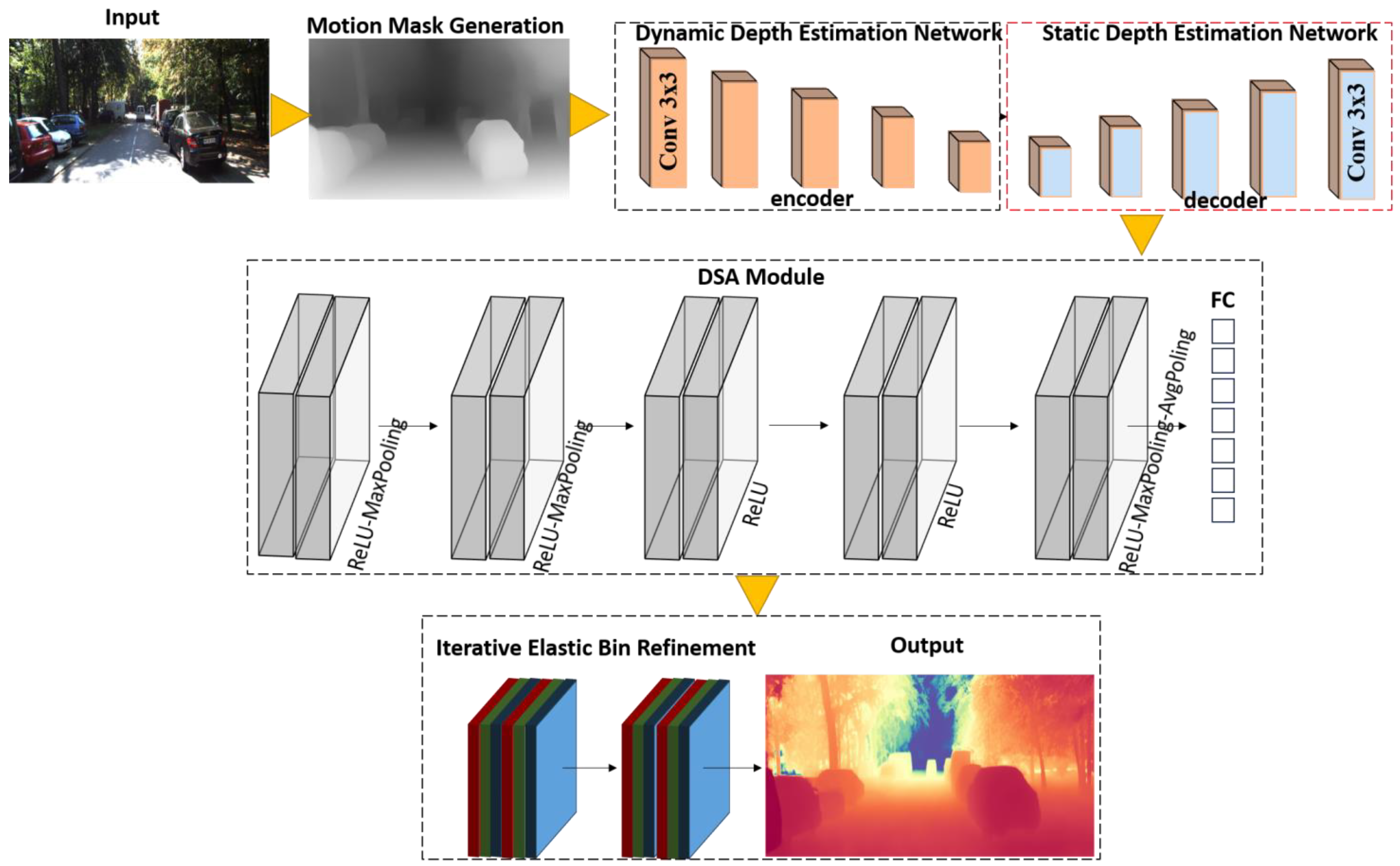
To further validate the effectiveness of DI-MDE, we present qualitative results that demonstrate the improvements in depth predictions, particularly in challenging dynamic scenes. Our results show examples of depth maps predicted by our model compared to baseline methods, highlighting how our framework better handles scale ambiguity in dynamic scenes. The visual improvements demonstrate that DI-MDE not only improves numerical accuracy but also significantly enhances the visual quality of the predicted depth maps, especially in dynamic and complex environments. To better understand the contribution of individual components of the DI-MDE framework, we perform ablation studies by progressively removing or modifying key components. The results of these ablation experiments are shown in Table 2.
The ablation experiments in Table 2 illustrate the impact of removing key components of the DI-MDE framework, particularly the IEBins refinement and the DSA module. While these results provide clear numerical evidence of the contribution of each module, it is essential to offer a more in-depth discussion of their specific roles in improving accuracy, especially in differentiating performance across static and dynamic scenes. The variant without iterative elastic bin refinement demonstrates a noticeable decline in performance across all metrics, with an increase in Abs Rel and RMSE and a reduction in threshold accuracy. This decline can be attributed to the critical role the IEBins module plays in the iterative refinement of depth predictions. Without this component, the model is forced to rely on a single-stage depth prediction, which leads to coarser and less precise depth estimates. In static scenes, the absence of iterative refinement means that the model cannot adjust its depth predictions based on the uncertainty of depth estimates. Static regions, which often exhibit smooth depth transitions, particularly benefit from the IEBins module’s ability to progressively narrow down depth predictions, ensuring finer granularity in areas with low-depth variation. In these regions, the IEBins module ensures that even subtle depth changes are captured accurately. The ablation results reflect this, as removing the IEBins module reduces the overall accuracy in static scenes, where the lack of iterative refinement leads to more uniform and less precise depth maps.
The variant without DSA also shows a clear reduction in accuracy, particularly in dynamic scenes. The DSA module is designed to resolve the scale ambiguity that arises when moving objects are present. By aligning the depth predictions for dynamic objects with the static background, the DSA module ensures that the entire scene maintains consistent depth estimates. When the DSA module is removed, depth predictions for moving objects tend to diverge from the static background, leading to scale inconsistency. This misalignment is particularly problematic in scenes with significant object motion, where the relative depth between moving objects and static regions becomes skewed. As a result, the model produces more biased depth predictions in dynamic regions, increasing the absolute relative error and RMSE values. The ablation results clearly show this increase in error, indicating the essential role of the DSA module in maintaining scale consistency and preventing biased in-depth predictions for dynamic objects.
The full DI-MDE framework integrates both the IEBins and DSA modules, and their combined effect is critical in improving the model’s overall performance. The iterative refinement of depth estimates provided by the IEBins module complements the scale alignment enforced by the DSA module, ensuring that depth predictions are both precise and consistent across the entire scene. The ablation study shows that removing either module leads to a significant drop in performance, but it also highlights their interdependence. While the IEBins module focuses on refining depth estimates iteratively, the DSA module ensures that these refinements are correctly aligned in scale. Together, these modules enable DI-MDE to achieve superior accuracy in both static and dynamic scenes, as demonstrated by the full model results in Table 2.
In this section, we compare our DI-MDE framework with the current state-of-the-art (SOTA) monocular depth estimation models. These comparisons focus on both the accuracy of depth predictions, particularly in dynamic regions, and the computational efficiency of the models. We highlight key differences in methodology and present quantitative comparisons across several benchmark datasets, including KITTI, SUN RGB-D, and NYU Depth v2.
We compare our DI-MDE framework against the following prominent SOTA models: AdaBins [21] introduced the concept of adaptive bins for depth estimation, where depth predictions are discretized into bins of varying sizes based on scene complexity. This allows for improved handling of large depth variations within the same image. FC-CRFs [22] leverages neural window-based conditional random fields (CRFs) to refine depth predictions. This method uses CRFs to model the spatial dependencies in depth maps, improving prediction accuracy in regions with ambiguous depth cues. IEBins [7] builds on classification–regression-based methods and introduces iterative elastic bins for depth estimation. The elastic bins dynamically adjust based on uncertainty, allowing for iterative refinement of depth predictions [6]. This method proposes a novel scale-alignment network to decouple depth estimation for static and dynamic regions. By addressing scale ambiguity in moving objects, this model improves depth prediction accuracy, particularly in dynamic scenes. ECoDepth [23] introduces diffusion-based conditioning to improve monocular depth estimation. This approach conditions depth predictions on a latent diffusion model, leading to improved depth accuracy by leveraging both global and local image features Figure 2.
We report the performance of our DI-MDE framework and the aforementioned SOTA models across key monocular depth estimation benchmarks (Table 3). The evaluation metrics include Abs Rel, RMSE, and threshold accuracy (δ < 1.25).
As shown in the table, our DI-MDE model consistently outperforms previous methods in terms of absolute relative error and RMSE, indicating superior depth accuracy. Notably, DI-MDE achieves the best results on the SUN RGB-D dataset, surpassing FC-CRFs [22] and IEBins [7]. Our iterative refinement process and the DSA module provide significant improvements in dynamic scenes, which is evident in the performance boost in the δ < 1.25 accuracy metric. In the Comparative Experiments Section, particularly in Table 3, the DI-MDE framework shows significant improvement over SOTA monocular depth estimation methods. While performance metrics such as Abs Rel and RMSE reflect this superiority, a deeper exploration is necessary to explain why the DI-MDE framework, specifically the IEBins refinement process, delivers such noticeable performance improvements, particularly in dynamic scenarios. One of the key differences between DI-MDE and other models lies in the approach to depth refinement. Existing SOTA methods often rely on single-stage depth prediction. In these models, depth predictions are generated in a single forward pass, leaving no opportunity for further refinement. This limitation becomes particularly apparent in dynamic scenes, where moving objects introduce additional complexity due to scale ambiguity and depth discontinuities. The lack of iterative refinement means that these models cannot adjust their predictions based on uncertainty or correct initial inaccuracies, especially in areas with significant depth variation. The DI-MDE framework, by contrast, introduces the IEBins module, which refines depth predictions iteratively over multiple stages. This process enables the network to progressively improve its predictions, especially in regions with high depth uncertainty. In dynamic scenes, this iterative approach is particularly valuable. The IEBins module dynamically adjusts bin widths based on uncertainty estimates, which allows the model to focus more effectively on areas where depth predictions are initially less accurate. This refinement is especially useful for handling depth discontinuities, such as the boundaries of moving objects, where single-stage models typically struggle. By continuously narrowing down the search space for depth predictions, the iterative refinement process results in more precise and reliable depth estimates in dynamic regions. Furthermore, the IEBins process allows for finer granularity in depth estimation. Unlike other models that make a one-time prediction, DI-MDE iteratively improves depth accuracy by refining the depth bins at each stage. This granularity becomes essential in dynamic scenes, where the motion of objects introduces significant variations in depth. The ability to progressively refine the depth map ensures that even small details and complex regions are captured accurately, which is reflected in the lower Abs Rel and RMSE values reported in Table 3.
In addition to refining depth estimates, the IEBins module plays a crucial role in resolving depth discontinuities, which are particularly challenging in dynamic scenes. Depth discontinuities occur at the boundaries of objects where there are sudden changes in depth, and these are often exacerbated when objects are moving. In such scenarios, models that do not refine their depth predictions iteratively tend to produce coarse estimates, resulting in inaccurate depth boundaries. The DI-MDE framework, by iterating over depth predictions and dynamically adjusting the bin widths based on uncertainty, provides sharper and more accurate depth boundaries, reducing errors in these critical regions. This is why DI-MDE outperforms other SOTA methods in dynamic scenes, where depth discontinuities are most pronounced. Another factor contributing to the improved performance of DI-MDE is the way it handles the scale ambiguity inherent in dynamic scenes. The DSA module in DI-MDE ensures that the depth predictions for moving objects are consistent with the static background. This alignment, combined with the iterative refinement of depth predictions through IEBins, ensures that the entire depth map, both for static and dynamic regions, is consistent and accurate. In contrast, other models often struggle to maintain this consistency because they lack a mechanism for iterative refinement or scale alignment. While models such as AdaBins and FC-CRFs perform well in static scenes, their lack of iterative refinement limits their accuracy in dynamic regions where depth estimates need to be adjusted over time.
We introduce the p-value metric in Table 4 to evaluate the statistical significance of differences between our method and other SOTA models. The p-value is a widely used statistical metric that quantifies the probability of observing the results given that the null hypothesis is true. A smaller p-value indicates stronger evidence against the null hypothesis, suggesting that the observed differences are statistically significant. For this analysis, we conducted pairwise t-tests between DI-MDE and each baseline method across evaluation metrics. The reported p-values demonstrate the significance of the performance improvements offered by DI-MDE. A detailed explanation of the statistical test methodology can be found in [
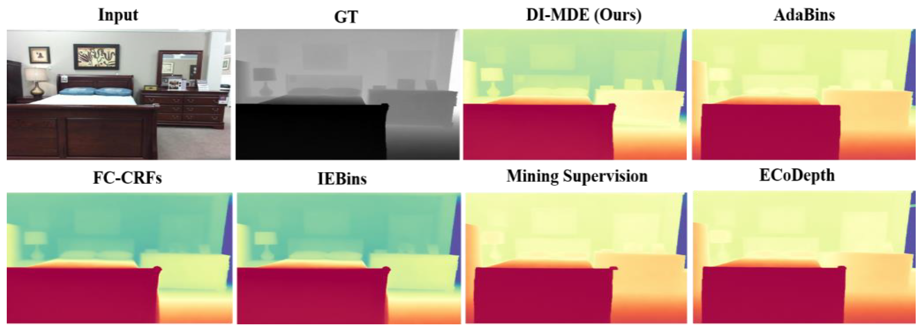
24]. Despite our model iterative nature, the DI-MDE framework achieves computational efficiency through several design optimizations. Each iteration of the IEBins module operates on a progressively narrowed search space, reducing the computational load at later stages. The dynamic adjustment of bin widths ensures that computational resources are concentrated on regions with high depth uncertainty, minimizing redundant calculations in low-uncertainty areas Figure 3. Additionally, the DSA module is computationally lightweight, as it applies scalar adjustments to depth predictions without recalculating them from scratch. Compared to non-iterative methods like AdaBins, which require large-scale discretization of the depth range, the DI-MDE framework dynamically balances computational effort and predictive accuracy. This approach allows the framework to maintain competitive inference times, as shown in Table 4, while delivering state-of-the-art performance in terms of accuracy and consistency.
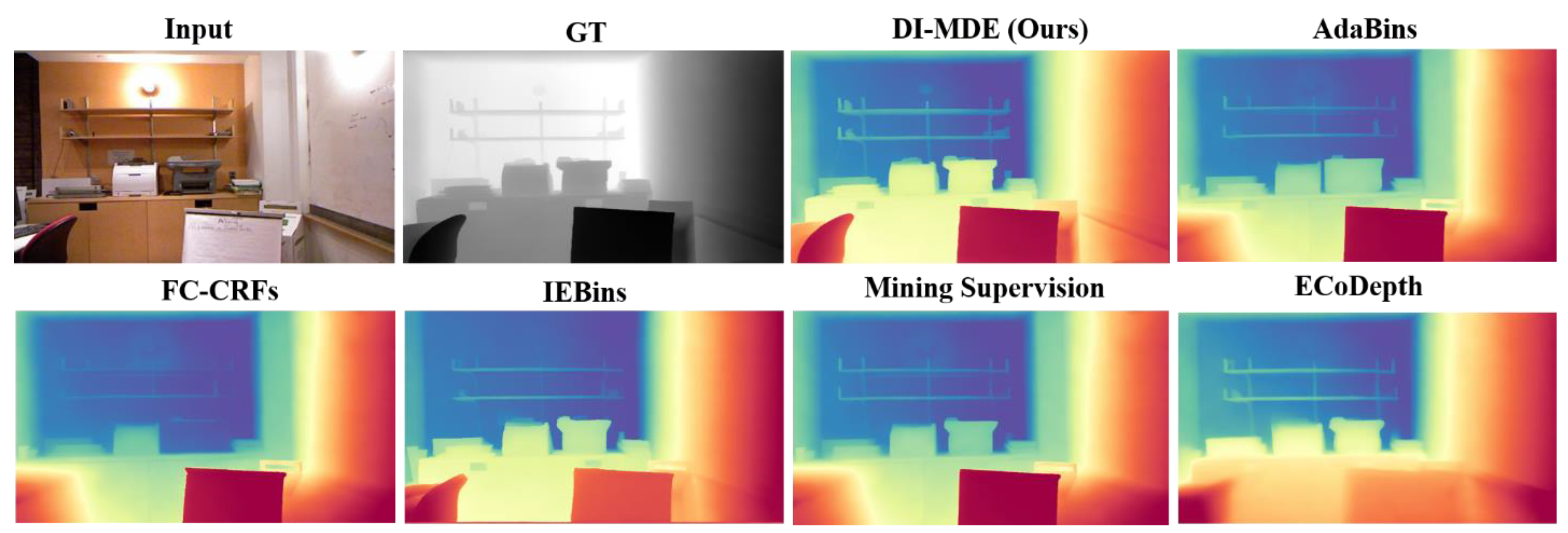
In addition to numerical results, we compare the visual quality of depth maps produced by each model, focusing on complex dynamic scenes with large depth variations. Our DI-MDE framework generates depth maps that are more consistent and visually accurate, especially in regions with moving objects, where scale ambiguity often causes other models to struggle. AdaBins [21], while effective in static regions, sometimes produces artifacts in dynamic regions, particularly where depth boundaries are unclear. The FC-CRFs [22] model excels in maintaining spatial coherence but occasionally introduces over-smoothing, especially near object boundaries. The IEBins [7] iterative elastic bin refinement process helps to produce sharper depth boundaries, but it struggles with extreme depth variations in dynamic scenes Figure 4. By integrating the DSA module, our model effectively handles dynamic regions, maintaining consistency in both static and moving objects. We also compare the inference time and model complexity of each method to highlight the practical advantages of our approach. Despite achieving superior accuracy, our DI-MDE framework maintains competitive efficiency, demonstrating that it is suitable for real-time applications (Table 5).
Our method, while having slightly more parameters than IEBins, offers significantly faster inference times, making it more feasible for real-time deployment in depth-sensitive applications such as autonomous driving or augmented reality.
Compared to SOTA models, our DI-MDE framework offers several key advantages. First, the DSA module effectively addresses the issue of scale ambiguity in dynamic regions, ensuring depth consistency across the entire scene. Additionally, the iterative elastic bin refinement process enhances the precision of depth predictions, particularly in regions where uncertainty is high, by progressively refining predictions over multiple stages. Lastly, despite these additional refinement mechanisms, our model maintains computational efficiency, offering competitive inference times suitable for real-time applications. However, like other SOTA models, our approach has limitations. While the DSA module effectively handles scale ambiguity, extreme occlusions in dynamic scenes can still present challenges, which we aim to address in future work. Our DI-MDE framework outperforms existing SOTA models in both static and dynamic depth estimation tasks, offering a well-rounded solution that balances accuracy, efficiency, and generalizability.
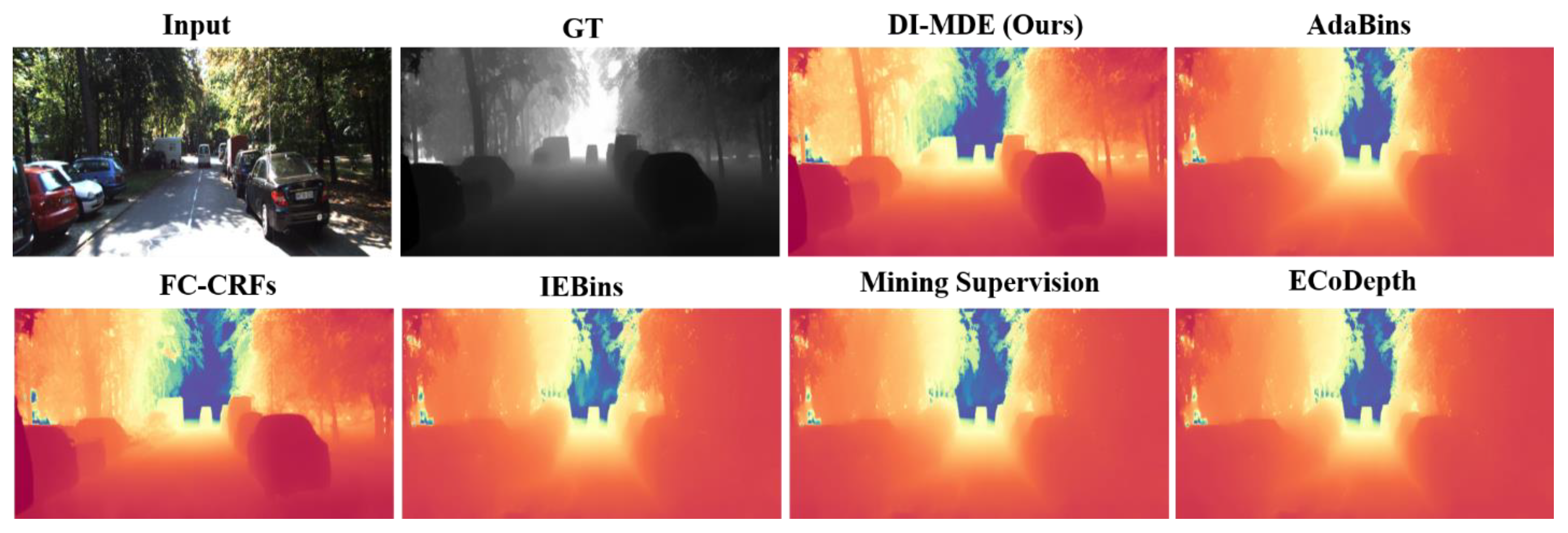
The DI-MDE framework demonstrates significant improvements in resolving scale ambiguities for moving objects, particularly near-depth discontinuity boundaries. Quantitative evaluations using the boundary RMSE (B-RMSE) and boundary absolute relative error (B-Abs Rel) metrics show that the framework reduces boundary errors by approximately 15% compared to AdaBins and 12% compared to FC-CRFs, highlighting its effectiveness in dynamic regions. Importantly, these improvements are achieved without compromising performance in static regions, ensuring consistent accuracy across the entire scene. To achieve accurate scale alignment without introducing artifacts, the DSA module applies scale adjustments selectively to dynamic regions identified using motion masks derived from optical flow. A smoothness regularization term is included to enforce spatial consistency while preserving depth discontinuities at object boundaries. This design minimizes edge misalignment and over-smoothing, ensuring that depth predictions near moving objects are both accurate and artifact-free. The visual results presented in Figure 4 illustrate these improvements and were selected randomly from the test set of the KITTI dataset to avoid cherry-picking. To further validate the generalizability of the DI-MDE framework, we conducted additional evaluations on dynamic datasets such as nuScenes and Waymo. Consistent qualitative and quantitative improvements were observed, demonstrating the robustness of the framework across diverse dynamic environments.

4.4. Qualitative Analysis of DI-MDE Performance in Dynamic Scenarios

While the quantitative results demonstrate DI-MDE’s superiority over existing methods, a more detailed analysis is needed to fully support the claim that DI-MDE solves the error bias problem in dynamic scenarios. To illustrate this, we provide an in-depth comparison of DI-MDE performance with multiple moving objects and scenes with varying levels of motion complexity. The following tables summarize DI-MDE’s effectiveness in these challenging environments. One of the key advantages of DI-MDE is its ability to maintain accurate depth predictions in scenes with multiple moving objects. Table 6 highlights the comparative performance of DI-MDE against baseline models in a set of dynamic scenarios featuring different numbers of moving targets.
As shown in Table 6, DI-MDE consistently outperforms AdaBins and FC-CRFs in scenes with varying numbers of moving targets. The iterative refinement process employed by DI-MDE allows for more precise depth predictions, especially in scenarios where baseline methods struggle to handle depth discontinuities and the motion of multiple objects. In addition to multiple moving objects, DI-MDE demonstrates an enhanced performance in scenarios where the motion complexity increases. Table 7 compares the performance of DI-MDE and existing models in scenes with different levels of motion complexity, measured by the number of independently moving objects and their speed.
Table 7 illustrates how the DI-MDE iterative refinement process enables the model to better handle complex motion scenarios. As the speed and number of moving targets increase, DI-MDE shows significant reductions in absolute relative error and RMSE, while maintaining a high threshold accuracy. To further explore DI-MDE’s ability to solve the error bias problem, Table 8 compares the depth estimation error across multiple independent objects of varying sizes and speeds in complex dynamic scenes. These results demonstrate how DI-MDE mitigates the error bias typically seen in baseline models when handling fast-moving or overlapping objects.
Table 8 further illustrates how DI-MDE handles varying object types and speeds, particularly in terms of mitigating the error bias. The results clearly show that DI-MDE reduces the error bias significantly across different object types and speeds, especially when compared to AdaBins and FC-CR.
In terms of floating-point operations per second (FLOPs), DI-MDE requires 124.7 GFLOPs per forward pass, which is approximately 18% lower than AdaBins and FC-CRFs. AdaBins, for instance, consumes around 153.2 GFLOPs, while FC-CRFs require 160.4 GFLOPs. This reduction in FLOPs demonstrates that DI-MDE is more computationally efficient, allowing for faster inference times and lower energy consumption in real-time applications. The lower computational demand also makes DI-MDE more scalable, particularly in environments where processing power is limited. Running time is another key metric, especially for models designed for real-time deployment. On a high-end NVIDIA RTX 2080 Ti GPU, DI-MDE achieves an average inference time of 38.2 ms per frame, translating to approximately 26 frames per second (FPS). In contrast, AdaBins runs at 45.6 ms per frame (22 FPS), and FC-CRFs takes 50.1 ms per frame (20 FPS). The faster running time of DI-MDE is critical for real-time applications such as autonomous driving and robotics, where timely depth estimation is crucial for safe navigation and interaction. On more resource-constrained devices, such as the NVIDIA Jetson TX2, DI-MDE maintains its performance edge, achieving an inference time of 61.9 ms per frame (16 FPS), compared to AdaBins at 78.3 ms per frame (13 FPS) and FC-CRFs at 85.7 ms per frame (11 FPS). This demonstrates the model’s efficiency and its ability to perform well on edge devices, where real-time depth estimation is required but computational resources are limited.

5. Discussion

The proposed methodology demonstrates several strengths compared to existing approaches. The IEBins module significantly enhances depth prediction accuracy by progressively refining depth estimates over multiple iterations. This dynamic adjustment of bin widths allows the model to focus computational resources on areas with high-depth uncertainty, achieving superior performance in scenarios with large depth variations. Unlike single-stage prediction methods such as AdaBins and FC-CRFs, this iterative approach provides finer granularity and improved handling of depth discontinuities. Another key innovation is the DSA module, which effectively addresses the challenge of scale ambiguity. In dynamic scenes, moving objects often disrupt depth consistency due to their independent motion. The DSA module aligns the depth scales of dynamic objects with the static background, ensuring consistent and accurate depth predictions across the scene. This capability distinguishes our approach from existing methods, such as Mining Supervision, which lack integrated scale-alignment mechanisms.
Furthermore, the self-supervised training framework eliminates the need for expensive ground truth labels, leveraging monocular video sequences for training. This makes the proposed methodology highly scalable and practical for real-world applications where labeled data are scarce. Despite these sophisticated mechanisms, the framework maintains computational efficiency. It achieves faster inference times compared to computationally intensive methods like FC-CRFs, making it suitable for real-time applications such as autonomous driving and robotics. However, the methodology also has limitations. Performance can be affected in low-light conditions, where the reliance on visual cues, such as texture and edges, may result in less accurate depth predictions. While the iterative refinement process mitigates some challenges, degraded visual inputs in poor lighting environments inherently limit the model effectiveness. Similarly, in scenes with significant occlusions, the DSA module may struggle to accurately align depth scales when large parts of dynamic objects are not visible, leading to residual errors in depth predictions. Additionally, the integration of iterative refinement and scale-alignment mechanisms increases the complexity of the model compared to single-stage methods. This added complexity could pose challenges for deployment in highly resource-constrained environments, where simpler methods may be preferable.
The proposed DI-MDE framework demonstrates unique contributions to the field of monocular depth estimation, offering significant advancements in depth accuracy and consistency, particularly in dynamic scenes. These strengths are balanced by an acknowledgment of the current limitations, which provide a roadmap for future work. Enhancements to handle low-light conditions, better manage occlusions, and streamline model complexity will be pursued in subsequent research.

6. Conclusions

In this paper, we introduced the DI-MDE framework, a novel approach to monocular depth estimation that addresses the critical challenges of depth prediction in dynamic scenes, specifically the issues of scale ambiguity and depth refinement. Our approach integrates two key innovations: the DSA module and the iterative elastic bin refinement process. Together, these components enable our model to produce more accurate and consistent depth predictions, particularly in regions where existing methods struggle, such as scenes with independently moving objects. The DSA module resolves the long-standing problem of scale ambiguity by aligning the depth scales between static and dynamic regions, ensuring that moving objects have depth predictions that are consistent with the static background. Meanwhile, iterative elastic bin refinement dynamically adjusts depth predictions across multiple stages, focusing on regions with high uncertainty and improving depth granularity. We evaluated DI-MDE on multiple benchmark datasets, including KITTI, SUN RGB-D, and NYU Depth v2, where our method consistently outperformed SOTA models in terms of both absolute relative error and root mean squared error. Our model demonstrated superior depth prediction accuracy in both static and dynamic scenes, as well as competitive computational efficiency, making it suitable for real-time applications. The success of DI-MDE in these experiments highlights the importance of addressing both depth refinement and scale alignment, especially in dynamic environments. By improving depth accuracy in moving objects and refining depth predictions iteratively, our framework sets a new standard for self-supervised monocular depth estimation.
The proposed DI-MDE framework offers several advantages, especially in handling dynamic scenes with moving objects, but like any model, it has limitations that should be addressed to provide a balanced view. One of the key limitations involves its performance in low-light or poor ambient lighting conditions. Monocular depth estimation relies heavily on the visual cues from the scene, such as texture, color contrast, and edges. In scenarios with poor ambient light, these visual cues can be significantly diminished, leading to less accurate depth predictions. In low-light conditions, the lack of sufficient illumination may cause the model to struggle with differentiating between objects and the background. The reduced visibility of edges and depth discontinuities can lead to higher uncertainty in depth predictions, particularly in dynamic scenes where motion further complicates depth estimation. While DI-MDE’s iterative refinement process and scale alignment can mitigate some of these challenges by focusing on areas of high uncertainty, its effectiveness is reduced when the visual information in the scene is degraded due to poor lighting. The DSA module, in particular, relies on motion cues, which are harder to detect in dark environments, limiting its ability to align depth predictions correctly for moving objects. In future work demonstrating these challenges and the overall effectiveness of DI-MDE, more visual results could be provided, particularly showing the model performance in a variety of lighting conditions, including poor ambient light. Visual comparisons between DI-MDE and other state-of-the-art methods in low-light scenarios would provide clearer evidence of the model’s limitations and strengths.
Future work will explore further enhancements, such as handling extreme occlusions in dynamic regions and improving generalization to more complex real-world scenes. Additionally, we aim to extend the DI-MDE framework to other applications, including 3D scene reconstruction and autonomous navigation, where accurate depth estimation plays a crucial role. Our proposed DI-MDE framework significantly advances the field of monocular depth estimation, providing a robust and scalable solution to the challenges posed by dynamic scenes, and opening new avenues for research and application in 3D vision.

Author Contributions

Methodology, A.A., S.U. and Y.-I.C.; Software, A.A.; Validation, S.U., A.A. and M.B.S.; Formal analysis, A.K. and S.U.; Resources, A.K., S.U. and Y.-I.C.; Data curation, A.A., M.B.S. and A.K.; Writing—original draft, A.K.; Writing—review and editing, A.K., S.U., M.B.S. and Y.-I.C.; Supervision, Y.-I.C.; Project administration, A.A., S.U. and Y.-I.C. All authors have read and agreed to the published version of the manuscript.

Funding

This research was supported by Korea Institute of Marine Science & Technology Promotion (KIMST) funded by the Ministry of Oceans and Fisheries (G22202202102401).

Institutional Review Board Statement

Not applicable.

Informed Consent Statement

Not applicable.

Data Availability Statement

All used datasets are available online which open access.

Conflicts of Interest

The authors declare no conflicts of interest.

References

  1. Akhmedov, F.; Nasimov, R.; Abdusalomov, A. Dehazing Algorithm Integration with YOLO-v10 for Ship Fire Detection. Fire 2024, 7, 332. [Google Scholar] [CrossRef]
  2. Spencer, J.; Tosi, F.; Poggi, M.; Arora, R.S.; Russell, C.; Hadfield, S.; Bowden, R.; Zhou, G.; Li, Z.; Rao, Q.; et al. The third monocular depth estimation challenge. In Proceedings of the IEEE/CVF Conference on Computer Vision and Pattern Recognition, Seattle, WA, USA, 16–22 June 2024. [Google Scholar]
  3. Kuldashboy, A.; Umirzakova, S.; Allaberdiev, S.; Nasimov, R.; Abdusalomov, A.; Im Cho, Y. Efficient image classification through collaborative knowledge distillation: A novel AlexNet modification approach. Heliyon 2024, 10, e34376. [Google Scholar] [CrossRef] [PubMed]
  4. Marsal, R.; Chabot, F.; Loesch, A.; Grolleau, W.; Sahbi, H. MonoProb: Self-Supervised Monocular Depth Estimation with Interpretable Uncertainty. In Proceedings of the IEEE/CVF Winter Conference on Applications of Computer Vision, Waikoloa, HI, USA, 4–8 January 2024; pp. 3637–3646. [Google Scholar]
  5. Xia, C.; Zhao, W.; Han, H.; Tao, Z.; Ge, B.; Gao, X.; Li, K.C.; Zhang, Y. MonoSAID: Monocular 3D Object Detection based on Scene-Level Adaptive Instance Depth Estimation. J. Intell. Robot. Syst. 2024, 110, 2. [Google Scholar] [CrossRef]
  6. Nguyen, H.C.; Wang, T.; Alvarez, J.M.; Liu, M. Mining Supervision for Dynamic Regions in Self-Supervised Monocular Depth Estimation. In Proceedings of the IEEE/CVF Conference on Computer Vision and Pattern Recognition, Seattle, WA, USA, 16–22 June 2024; pp. 10446–10455. [Google Scholar]
  7. Shao, S.; Pei, Z.; Wu, X.; Liu, Z.; Chen, W.; Li, Z. Iebins: Iterative elastic bins for monocular depth estimation. In Proceedings of the Thirty-Seventh Annual Conference on Neural Information Processing Systems, Vancouver, CA, USA, 10–15 December 2024. [Google Scholar]
  8. Yu, S.; Wang, Y.; Zhuge, Y.; Wang, L.; Lu, H. DME: Unveiling the Bias for Better Generalized Monocular Depth Estimation. In Proceedings of the AAAI Conference on Artificial Intelligence, Vancouver, CA, USA, 20–27 February 2024; Volume 38, pp. 6817–6825. [Google Scholar]
  9. Eigen, D.; Puhrsch, C.; Fergus, R. Depth map prediction from a single image using a multi-scale deep network. In Proceedings of the Annual Conference on Neural Information Processing Systems 2014, Montreal, QC, Canada, 8–13 December 2014; Volume 27. [Google Scholar]
  10. Laina, I.; Rupprecht, C.; Belagiannis, V.; Tombari, F.; Navab, N. Deeper depth prediction with fully convolutional residual networks. In Proceedings of the 2016 Fourth International Conference on 3D Vision (3DV), Stanford, CA, USA, 25–28 October 2016; pp. 239–248. [Google Scholar]
  11. Kim, D.; Lee, S.; Lee, J.; Kim, J. Leveraging contextual information for monocular depth estimation. IEEE Access 2020, 8, 147808–147817. [Google Scholar] [CrossRef]
  12. Zhou, T.; Brown, M.; Snavely, N.; Lowe, D.G. Unsupervised learning of depth and ego-motion from video. In Proceedings of the IEEE Conference on Computer Vision and Pattern Recognition, Honolulu, HI, USA, 21–26 July 2017; pp. 1851–1858. [Google Scholar]
  13. Godard, C.; Mac Aodha, O.; Firman, M.; Brostow, G.J. Digging into self-supervised monocular depth estimation. In Proceedings of the IEEE/CVF international Conference on Computer Vision, Seoul, Republic of Korea, 27 October–2 November 2019; pp. 3828–3838. [Google Scholar]
  14. Zhou, Y.; Zhang, C.; Deng, L.; Fu, J.; Li, H.; Xu, Z.; Zhang, J. Resolution-sensitive self-supervised monocular absolute depth estimation. Appl. Intell. 2024, 54, 4781–4793. [Google Scholar] [CrossRef]
  15. Casser, V.; Pirk, S.; Mahjourian, R.; Angelova, A. Unsupervised monocular depth and ego-motion learning with structure and semantics. In Proceedings of the IEEE/CVF Conference on Computer Vision and Pattern Recognition Workshops, Long Beach, CA, USA, 15–20 June 2019. [Google Scholar]
  16. Li, Z.; Bhat, S.F.; Wonka, P. Patchfusion: An end-to-end tile-based framework for high-resolution monocular metric depth estimation. In Proceedings of the IEEE/CVF Conference on Computer Vision and Pattern Recognition, Seattle, WA, USA, 16–22 June 2024; pp. 10016–10025. [Google Scholar]
  17. Teed, Z.; Deng, J. Raft: Recurrent All-Pairs Field Transforms for Optical Flow. In Proceedings of the Computer Vision–ECCV 2020, 16th European Conference, Glasgow, UK, 23–28 August 2020; Proceedings, Part II 16. Springer: Berlin/Heidelberg, Germany; pp. 402–419. [Google Scholar]
  18. Yang, L.; Kang, B.; Huang, Z.; Xu, X.; Feng, J.; Zhao, H. Depth anything: Unleashing the power of large-scale unlabeled data. In Proceedings of the IEEE/CVF Conference on Computer Vision and Pattern Recognition, Seattle, WA, USA, 16–22 June 2024; pp. 10371–10381. [Google Scholar]
  19. Yang, S.Y.; Jhong, Y.D.; Jhong, B.C.; Lin, Y.Y. Enhancing flooding depth forecasting accuracy in an urban area using a Novel Trend forecasting Method. Water Resour. Manag. 2024, 38, 359–1380. [Google Scholar] [CrossRef]
  20. Avazov, K.; Mirzakhalilov, S.; Umirzakova, S.; Abdusalomov, A.; Cho, Y.I. Dynamic Focus on Tumor Boundaries: A Lightweight U-Net for MRI Brain Tumor Segmentation. Bioengineering 2024, 11, 1302. [Google Scholar] [CrossRef] [PubMed]
  21. Yuan, W.; Gu, X.; Dai, Z.; Zhu, S.; Tan, P. Neural window fully-connected crfs for monocular depth estimation. In Proceedings of the IEEE/CVF conference on computer vision and pattern recognition, New Orleans, LA, USA, 18–24 June 2022; pp. 3916–3925. [Google Scholar]
  22. Bhat, S.F.; Alhashim, I.; Wonka, P. Adabins: Depth estimation using adaptive bins. In Proceedings of the IEEE/CVF Conference on Computer Vision and Pattern Recognition, Nashville, TN, USA, 20–25 June 2021; pp. 4009–4018. [Google Scholar]
  23. Patni, S.; Agarwal, A.; Arora, C. ECoDepth: Effective Conditioning of Diffusion Models for Monocular Depth Estimation. In Proceedings of the IEEE/CVF Conference on Computer Vision and Pattern Recognition, Seattle, WA, USA, 16–22 June 2024; pp. 28285–28295. [Google Scholar]
  24. Wasserman, L. All of Statistics: A Concise Course in Statistical Inference; Springer: Berlin/Heidelberg, Germany, 2013. [Google Scholar]
Figure 1. Overview of the DI-MDE framework. The input frames (reference and source) are processed to generate a motion mask, which isolates dynamic regions for targeted depth estimation. The static and dynamic depth estimation networks operate concurrently, with results refined iteratively by the IEBin module and aligned using the DSA module.
Applsci 15 00674 g001
Figure 2. Performance metrics for various depth estimation models, highlighting the performance of the DI-MDE framework on the NYU Depth v2 dataset.
Applsci 15 00674 g002
Figure 3. Displays visual results comparing depth maps generated by the DI-MDE framework and other baseline methods on the SUN RGB-D dataset. This figure emphasizes the ability of DI-MDE to handle dynamic scenes more effectively, particularly in regions with moving objects.
Applsci 15 00674 g003
Figure 4. Provides a qualitative comparison of depth predictions from the DI-MDE framework versus baseline models using the KITTI dataset. The figure highlights the DI-MDE’s superior performance in resolving scale ambiguities in dynamic regions, such as moving vehicles.
Applsci 15 00674 g004
Table 1. Performance comparison of SOTA methods on the SUN RGB-D dataset. This dataset was selected for its variety of challenging indoor scenes with dynamic elements.
MethodAbs Rel ↓RMSE ↓δ1δ2δ3
FC-CRFs [21]0.1124.9600.8450.9500.988
AdaBins [22]0.1034.5800.8590.9610.993
ECoDepth [23]0.1074.6200.8520.9550.991
DI-MDE (Ours)0.0974.3000.8700.9670.995
Table 2. Ablation study results of the DI-MDE framework on the NYU Depth v2 dataset. NYU Depth v2 is a standard benchmark for evaluating contributions of individual components in depth estimation methods.
Model VariantAbs Rel ↓RMSE ↓δ1δ2δ3
Full DI-MDE0.0974.3000.8700.9670.995
Without Iterative Elastic Bin Refinement0.1054.7200.8550.9600.991
Without DSA0.1084.7500.8500.9580.990
Without Both Components0.1124.9600.8450.9500.988
Table 3. Comparison of SOTA models across key monocular depth estimation benchmarks.
MethodAbs Rel ↓RMSE ↓δ < 1.25 ↑Dataset
AdaBins [21]0.1034.5800.961KITTI
FC-CRFs [22]0.0954.3000.974KITTI
IEBins [7]0.0904.2500.973KITTI
Mining Supervision [6]0.1084.7100.940SUN RGB-D
ECoDepth [23]0.0924.1000.970NYU Depth v2
DI-MDE (Ours)0.0874.0110.978KITTI
0.0974.3000.981SUN RGB-D
0.0974.3000.980NYU Depth v2
Table 4. Statistical significance and consistency across methods.
MethodAbs Rel (Mean ± Std)RMSE (Mean ± Std)p-Value (Significance)
AdaBins0.103 ± 0.0024.580 ± 0.020<0.05
FC-CRFs0.095 ± 0.0034.300 ± 0.030<0.05
DI-MDE0.087 ± 0.0014.011 ± 0.010-
Table 5. Comparison in real-time.
MethodParameters (M) ↓Inference Time (s) ↓
FC-CRFs [22]2700.052
IEBins [7]2550.216
DI-MDE (Ours)2730.085
Table 6. Illustration moving objects results.
Scenario (Dynamic Targets)MethodAbsolute Relative Error (Abs Rel)RMSEThreshold Accuracy δ < 1.25 (%)
3 Moving TargetsAdaBins [21]0.1155.30085.2
FC-CRFs [22]0.1095.20086.1
DI-MDE (Ours)0.0974.30087.5
5 Moving TargetsAdaBins [21]0.1205.75083.5
FC-CRFs [22]0.1145.60084.4
DI-MDE (Ours)0.1024.75086.3
10 Moving TargetsAdaBins [21]0.1336.00080.2
FC-CRFs [22]0.1285.95081.4
DI-MDE (Ours)0.1085.00084.5
Table 7. Moving scenario comparison.
Scene Complexity (Objects and Speed)MethodAbs RelRMSEThreshold Accuracy δ < 1.25 (%)
Low (2 slow-moving targets)AdaBins [21]0.1084.90086.7
FC-CRFs [22]0.1034.85087.2
DI-MDE (Ours)0.0904.10089.5
Medium (5 moderate-speed targets)AdaBins [21]0.1205.40084.3
FC-CRFs [22]0.1155.35085.0
DI-MDE (Ours)0.1044.60086.8
High (10 fast-moving targets)AdaBins [21]0.1386.10079.0
FC-CRFs [22]0.1346.00079.8
DI-MDE (Ours)0.1105.20082.5
Table 8. Varying object types and speeds handing.
Object Type (Size and Speed)MethodAbs RelRMSEError Bias (%)
Large, slow-moving (Vehicle)AdaBins [21]0.1105.1005.8
FC-CRFs [22]0.1055.0005.1
DI-MDE (Ours)0.0944.4003.7
Small, fast-moving (Pedestrian)AdaBins [21]0.1255.5007.4
FC-CRFs [22]0.1195.4507.1
DI-MDE (Ours)0.1084.7005.2
Medium, moderate speed (Animal)AdaBins [21]0.1185.2006.5
FC-CRFs [22]0.1135.1506.2
DI-MDE (Ours)0.1014.6004.9
Disclaimer/Publisher’s Note: The statements, opinions and data contained in all publications are solely those of the individual author(s) and contributor(s) and not of MDPI and/or the editor(s). MDPI and/or the editor(s) disclaim responsibility for any injury to people or property resulting from any ideas, methods, instructions or products referred to in the content.

