Aggregatable Subvector Commitment with Efficient Updates

Abstract

An aggregatable subvector commitment scheme extends a vector commitment scheme by enabling the aggregation of multiple proofs into a single compact subvector proof. However, the existing schemes have to recompute proofs for each position when inserting an element into the vector, incurring significant computational overhead. In this paper, we propose a novel aggregatable subvector commitment scheme based on Newton interpolation, which efficiently supports the addition of new elements. Specifically, the proposed scheme allows incremental updates to the commitment and proofs for each position, avoiding the requirement for full recomputation and thereby significantly reducing computational overhead. Additionally, we employ the Karatsuba algorithm to efficiently perform large-integer multiplication, which improves the aggregation and verification of proofs. Finally, we implement the proposed scheme and conduct a detailed comparison with aSVC. Experimental results demonstrate that the proposed scheme achieves a 48× speedup when adding an element to a 16-length vector, as well as 2.13× and 1.73× speedups for aggregating eight proofs and performing verification, respectively.

1. Introduction

Vector commitment (VC) [1,2,3,4,5,6,7,8,9,10,11,12,13,14] allows the committer to submit an ordered sequence of messages $\mathbf{v}=(v_0,v_1,v_2,\cdots ,v_{n-1})$ of size n, generate a commitment value C that contains all the messages for which we cannot tell whether the commitment value C is generated for $(v_0,v_1,v_2,\cdots ,v_{n-1})$ or for $(v_0^{\prime },v_1^{\prime },v_2^{\prime },\cdots ,v_{n-1}^{\prime })$, and also to generate its location proof $({\pi }_0,{\pi }_1,{\pi }_2,\cdots ,{\pi }_{n-1})$ for each position of the message at the location. When a verifier wants to check if a specific message $v_i$ is at the i-th position, the committer sends the proof ${\pi }_i$, the commitment value C, and the message $v_i$. The verifier uses this information to validate the location proof ${\pi }_i$. If the verification is successful, it confirms that $v_i$ is indeed located at the i-th position.

VC is an efficient cryptographic tool that protects the privacy and integrity of data, and thus, has a wide range of potential applications in several fields. For example, in the field of blockchain technology, VC can protect user privacy and verify the validity of transactions. In particular, in the VC [3]-based stateless cryptocurrency system, the verifier only needs to store the vector commitment of the user’s account balance without maintaining the state of the entire ledger. When a user initiates a transfer, he/she only needs to submit the transaction and prove his/her account balance, and the validator will verify the correctness of the balance upon receiving the transaction, and if the validation passes, the transaction proceeds normally. Additionally, in the context of cloud storage, vector commitments [9] enable users to generate compact proofs for their uploaded data, allowing cloud service providers to verify data integrity efficiently. This approach significantly reduces storage requirements and communication overhead compared to conventional methods. Vector commitments also exhibit substantial utility in the domains of zero-knowledge proofs. Specifically, within zero-knowledge proof [1,15,16,17] protocols, they enable the prover to demonstrate the satisfaction of specific set conditions without disclosing additional information. This is particularly valuable in large-scale data analytics or machine learning applications, where vector commitments can validate the participation of individual data points or the accuracy of computational outcomes, thereby enhancing the overall credibility of data processing procedures.

In order to improve the efficiency of verification, some commitment schemes [3,8,9,10] introduce the concept of subvector, i.e., multiple proofs of transactions can be aggregated into a concise single proof, thus further reducing the verification overhead. After the verification passes, we need to update the account status and its proofs in a timely manner in order to improve the updating efficiency. Thus, some scholars have proposed new vector commitment schemes [5,6,7], aiming to improve the efficiency of such updating. However, the existing VC schemes mainly focus on vectors of fixed size. When a new value is appended to the vector, the client has to recompute the commitment and proofs for all positions, leading to significant computational overhead. In this work, we explore an efficient aggregatable subvector commitment scheme that supports the dynamic addition of new values.

1.1. Our Contributions

In this paper, we propose a new aggregatable subvector commitment vector based on Newton interpolation, which can efficiently update the commitment and proofs when inserting a new value into the vector. Table 1 provides a brief comparison with previous research work. Our primary contributions can be outlined as follows:

Table 1. Comparison with previous work using aSVC.

Scheme	$\left|\mathit{C}\right|$	$|{\mathit{\pi }}_{\mathit{I}}|$	Aggregate	Verify $|{\mathit{\pi }}_{\mathit{i}}|$	Verify $|{\mathit{\pi }}_{\mathit{I}}|$	UpdateAllProofs	AddAllProofs
aSVC	$1|{\mathbb{G}}_1|$	$1|{\mathbb{G}}_1|$	$O(k{log}^{2}k)$	1	$O(k{log}^{2}k)$	$O(n)$	$O((n+l)log(n+l))$
Our Scheme	$1|{\mathbb{G}}_1|$	$1|{\mathbb{G}}_1|$	$O\left(1.39{({\displaystyle \frac{k}{2}}+1)}^{{log}_{2}3}\right)$	1	$O\left(1.39{({\displaystyle \frac{k}{2}}+1)}^{{log}_{2}3}\right)$	$O(n^2)$	$O(n+l^2)$

n is the vector size and k is the subvector size. All schemes have $O(n)$-sized parameters, $\left|C\right|$ is the commitment size of a vector of length n. UpdateAllProofs refers to the time required to update all proofs following a modification to a single element within a vector. AddAllProofs is the time it takes to update all the other proofs when we add a vector element and to compute the proof of the position of the newly added element, where l is the number of nodes added.

• This paper proposes a novel aggregatable subvector commitment scheme based on Newton interpolation. When appending a value to the vector, it eliminates the need to fully recompute the original commitment value and proofs. Instead, the client incrementally updates the commitment and proofs for each position, significantly reducing computational overhead.
• The Karatsuba algorithm can efficiently perform large-integer multiplication, which can reduce the computational overhead from $O(n^2)$ to $O(n^{{log}_{2}3})$ for the multiplication of two n-digit numbers. By leveraging this algorithm, our scheme improves the efficiency of both aggregation and verification operations.
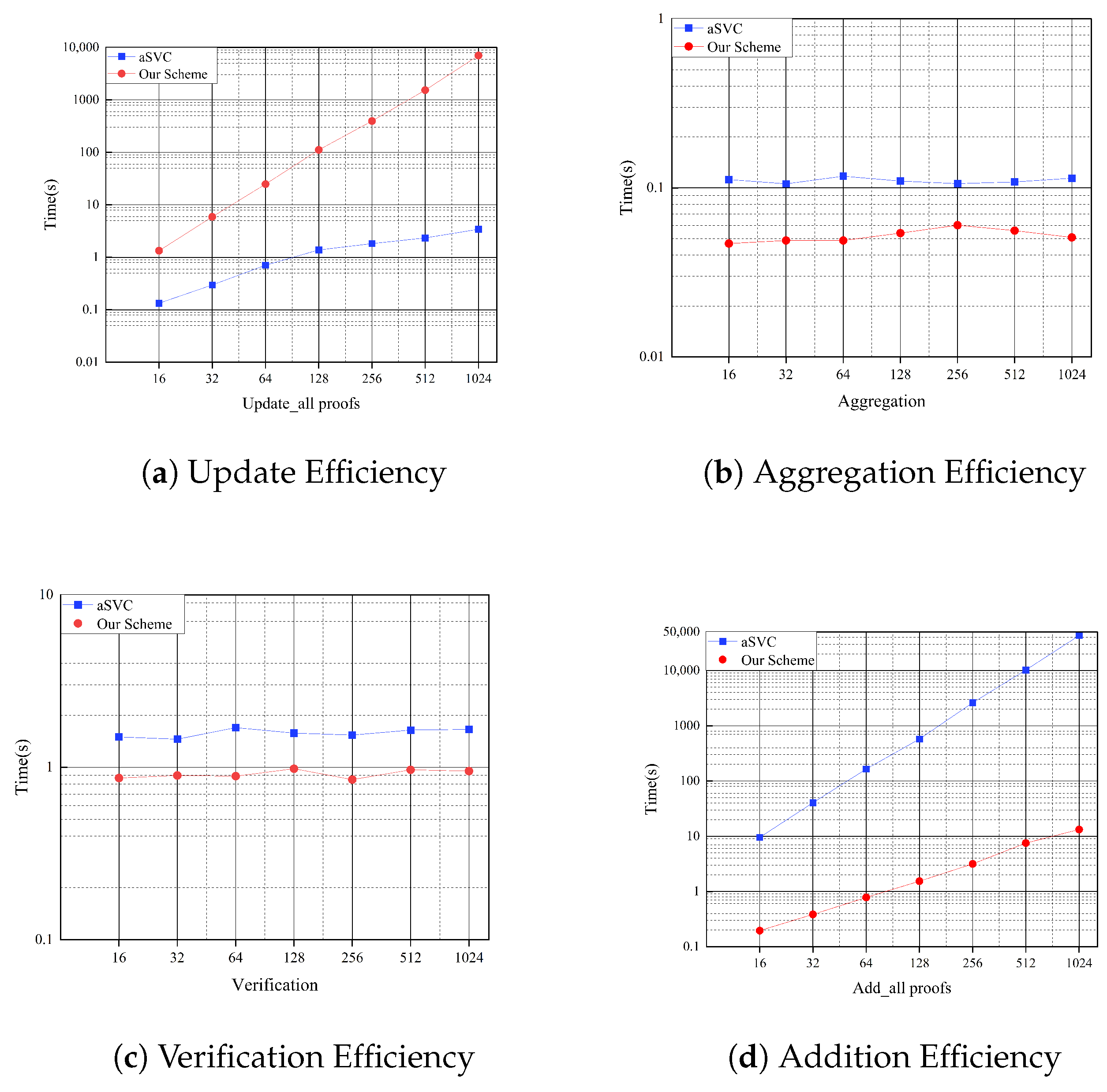
• We present a formal security analysis to prove that our scheme can achieve the security of position binding. Furthermore, we provide a thorough implementation, and the experiment results demonstrate that our scheme is more efficient at aggregation and verification, and at updating the proofs when appending a new value. Specifically, compared with aSVC, the proposed scheme achieves a 48× speedup when adding an element to a 16-length vector, as well as 2.13× and 1.73× speedups for aggregating eight proofs and performing verification, respectively.

1.2. Related Work

Vector commitment is a new cryptographic primitive first proposed by the authors of [1,15,16] as an alternative to Merkle trees [18]. It has several attractive properties, such as compactness, constant-size proofs, and the ability to aggregate multiple proofs into a single constant-size proof. Catalano et al. [2] constructed two vector commitment schemes based on the CDH and RSA assumptions. Although both can achieve the basic functions of commitment and proof, the RSA-based scheme still has room for improvement in aggregation efficiency. Lai et al. [8] further studied the new features of vector commitments and proposed subvector commitments (SVCs) that support opening commitments on arbitrary subsets of positions, and its proof size is related to the number of opened elements. In order to make SVCs more efficient and suitable for distributed systems, Campanelli et al. [9] proposed a new feature of vector commitments based on batch opening, namely incremental aggregation, that supports unlimited proof aggregation. This method allows the already aggregated proofs to continue to aggregate. They designed two implementations based on unknown-order groups, which are similar to the scheme proposed by Boneh et al. [10], and both implement constant-size public parameters, commitments and proofs, but the authors of [10] only support single-hop aggregation. Tomescu et al. proposed the aSVC [3] scheme based on KZG [1], which uses a polynomial method to calculate the aggregation proof, and can simultaneously realize batch opening and aggregation of proofs, but the aggregation efficiency needs to be improved. Hyperproofs proposed by Srinivasan et al. [5] is also based on polynomials, but its aggregation algorithm uses the IPA [19] proof system, and the actual aggregation overhead is large. In order to improve the efficiency of aggregation, Wang et al. [6] proposed BalanceProofs, which takes aSVC [3] as input and outputs a scheme with higher aggregation efficiency, but the aggregation efficiency of this scheme is still not ideal. In order to further optimize the efficiency of the aggregation algorithm, this paper proposes an improved scheme based on the polynomial calculation aggregation proof method, and combines the idea of the Karatsuba algorithm to implement an efficient aggregation algorithm.

In addition, the previous polynomial commitment scheme [1,3,5,6,13] will incur a lot of computational overhead if the data set is to be dynamically increased. In order to meet the above requirements, this paper proposes a new vector commitment scheme, which uses a combination of Newton interpolation and the Karatsuba algorithm to construct an efficient and aggregatable vector commitment scheme for dynamic data sets.

1.3. Organization

The sections of this paper are arranged as follows: Section 1 introduces the backgound, contributions and related work. Section 2 provides the relevant tools for constructing the scheme, including Newton interpolation, Karatsuba algorithm, and bilinear pairing. Section 3 explains the construction of the proposed vector commitment scheme. Section 4 gives the security analysis of our scheme. The simulation results and discussions are presented in Section 5. Finally, the conclusion is given in Section 6.

2. Preliminaries

This section will give the required symbols and briefly introduce some preliminaries, such as Newton interpolation, bilinear map, vector commitment and Karatsuba algorithm.

Notation. Here is the mathematical notation used in this paper: let $\lambda$ be a security parameter, $\mathit{negl}(·)$ be a negligible function, and $poly(·)$ be any function upper-bounded by some univariate polynomial. The vector $\mathbf{v}=(v_0,v_1,v_2,\dots ,v_{n-1})$ contains n elements, where each element $v_i\in {\mathbb{Z}}_p$ [20].

2.1. Newton Interpolation

Given n interpolation points $(x_0,v_0),(x_1,v_1),\cdots ,(x_{n-1},v_{n-1})$, where no two $x_i$ are the same, the Newton interpolation polynomial is a linear combination of Newton basis polynomial. We can express the Newton interpolation function as follows:

$$N(x)=\sum _{i\in [0,n)}{a}_i·w_i(x).$$

(1)

We denote the i-th basis polynomial of the Newton interpolating polynomials [21] as

$$w_i(x)=\prod _{j=0}^{i-1}(x-x_j),$$

(2)

where $w_0(x)=1$. The coefficients are defined as

$$a_i=[v_0,v_1,v_2,\cdots ,v_i],$$

(3)

where $[v_0,v_1,v_2,\cdots ,v_i]$ is the notation for the difference quotient, and the specific calculation process is as follows:

$$\begin{array}{cc}\hfill & a_0=[v_0]=v_0\hfill \\ \hfill & a_1=[v_0,v_1]={\displaystyle \frac{v_1-v_0}{x_1-x_0}}\hfill \\ \hfill & a_2=[v_0,v_1,v_2]={\displaystyle \frac{[v_1,v_2]-[v_0,v_1]}{x_2-x_0}}\hfill \\ \hfill & a_3=[v_0,v_1,v_2,v_3]={\displaystyle \frac{[v_1,v_2,v_3]-[v_0,v_1,v_2]}{x_3-x_0}}\hfill \\ \hfill & a_4=[v_0,v_1,v_2,v_3,v_4]={\displaystyle \frac{[v_1,v_2,v_3,v_4]-[v_0,v_1,v_2,v_3]}{x_4-x_0}}\hfill \\ \hfill & \cdots \hfill \\ \hfill & a_{n-1}=[v_0,v_1,v_2,\cdots ,v_{n-1}]={\displaystyle \frac{[v_1,v_2,\cdots ,v_{n-1}]-[v_0,v_1,\cdots ,v_{n-2}]}{x_{n-1}-x_0}}\hfill \end{array}$$

(4)

Therefore, the Newtonian polynomials are expanded in the following form:

$$N(x)=[v_0]+[v_0,v_1](x-x_0)+\cdots +[v_0,v_1,\cdots ,v_{n-1}](x-x_0)(x-x_1)\cdots (x-x_{n-2}).$$

(5)

We can see that $\forall i\in [0,n),N(x_i)=v_i$.

Both Newton interpolation and Lagrange interpolation are classic interpolation methods, but Newton interpolation has unique advantages. It uses the difference quotient form to gradually construct the interpolation polynomial, which has computational superiority; when a new interpolation point needs to be added, the previously calculated difference quotient result can be directly used, and only the newly added high-order difference quotient terms need to be calculated, thus avoiding the cost of complete recalculation. This progressive construction feature makes Newton interpolation particularly efficient when dealing with dynamically growing data sets. In contrast, Lagrange interpolation requires reconstructing all basis functions for each new point added.

2.2. Bilinear Pairing

We denote the parameters associated with the pairing by using $(p,e,{\mathbb{G}}_1,{\mathbb{G}}_2,{\mathbb{G}}_T,g_1,g_2)$. In particular, ${\mathbb{G}}_1,{\mathbb{G}}_2$ and ${\mathbb{G}}_T$ are all groups of order prime p, where $g_i$ is the generator of ${\mathbb{G}}_i$. Define e as ${\mathbb{G}}_1\times {\mathbb{G}}_2\to {\mathbb{G}}_T$ to be a bilinear pairing that satisfies the following properties [22,23,24,25]:

• Bilinearity: $\forall u\in {\mathbb{G}}_1,w\in {\mathbb{G}}_2$ and $a,b\in {\mathbb{Z}}_p$ it is $e(u^a,w^b)=e{(u,w)}^{ab}$.
• Non-degeneracy: $e(g_1,g_2)\ne 1$.
• Computable: For all $u\in {\mathbb{G}}_1,w\in {\mathbb{G}}_2$, we have an efficient algorithm to compute $e(u,w)$.

To simplify the description of the protocol, we consider ${\mathbb{G}}_1$ and ${\mathbb{G}}_2$ as the same group $\mathbb{G}$ and use the same generating element g.

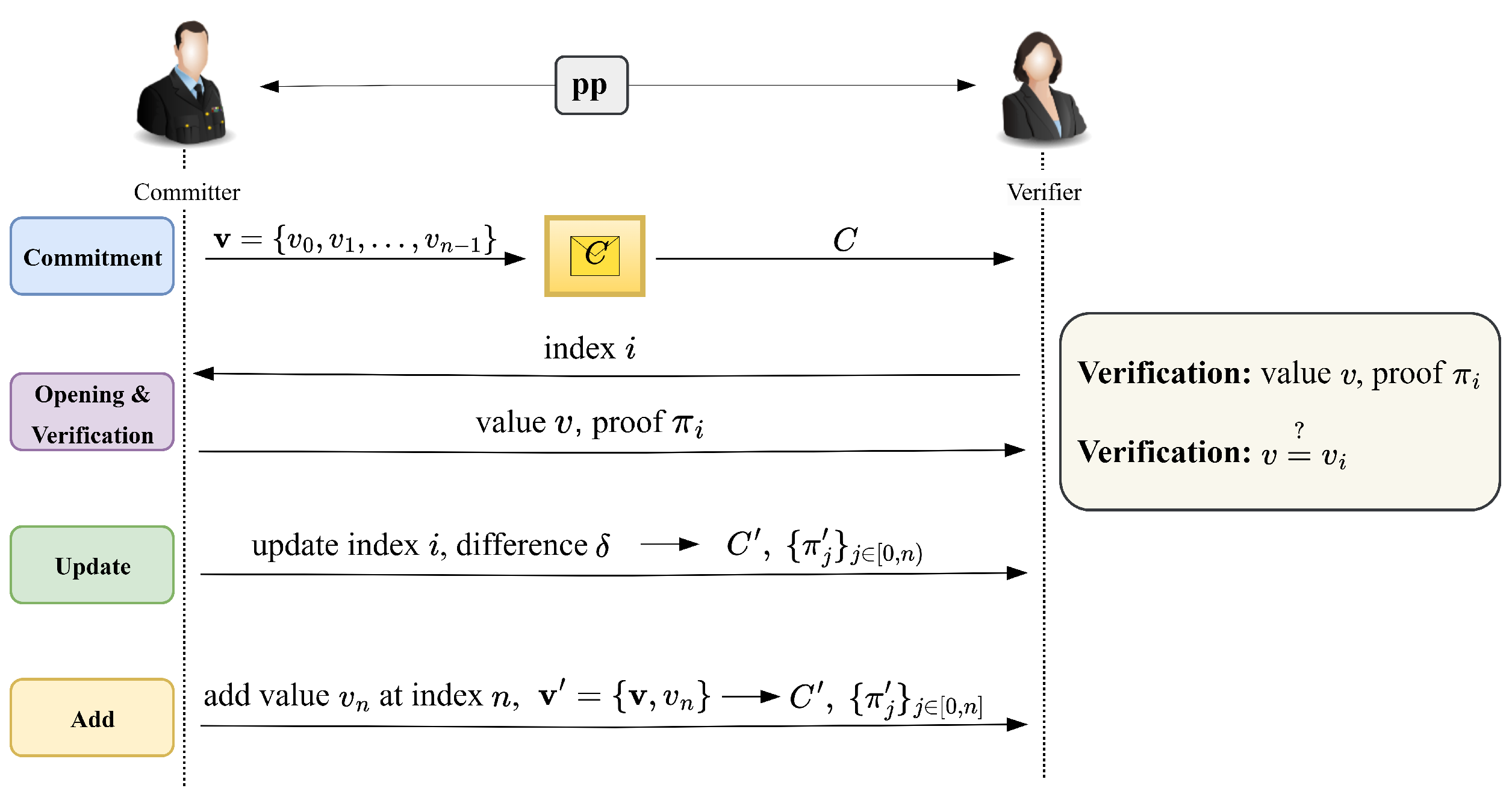
2.3. Vector Commitment

Informally, VC allows the submission of an ordered sequence of values that can be subsequently verified against a specific position. We recall a formal definition of vector commitment in Hyperproofs [5].

Definition 1 (VC).

A VC scheme is a set of the following nine PPT algorithms:

• Gen$(1^{\lambda },n)\to$ pp: Inputting vector size n and security parameter λ outputs the public parameters.
• Commit(pp,$\mathbf{v}$) → (C,aux): Inputting vector $\mathbf{v}=\{v_0,v_1,\cdots ,v_{n-1}\}$ outputs commitment C and auxiliary information $\mathsf{aux}$.
• Open(pp, i,$\mathbf{v}$, aux) $\to {\pi }_i$: Inputting the position index i, the vectors $\mathbf{v}$ and $\mathsf{aux}$ outputs proof ${\pi }_i$ at index i.
• OpenAll(pp, $\mathbf{v}$) $\to \{{\pi }_0,{\pi }_1,{\pi }_2,\cdots ,{\pi }_{n-1}\}$: Inputting vector $\mathbf{v}$ outputs proofs at all positions ${\pi }_0,{\pi }_1,\cdots ,{\pi }_{n-1}$.
• Agg(pp,$I,{({\pi }_i,v_i)}_{i\in I})\to {\pi }_I$: For the aggregate set $I\subseteq [0,n)$, inputting the proofs ${\left\{{\pi }_i\right\}}_{i\in I}$ and the values ${\left\{v_i\right\}}_{i\in I}$ outputs ${\pi }_I$, which is an aggregated proof of constant size.
• Verify(pp, C, $I,{\left\{v_i\right\}}_{i\in I},{\pi }_I):=\{0,1\}$: Inputting values ${\left\{v_i\right\}}_{i\in I}$, commitment C and aggregate proof ${\pi }_I$ outputs either 0 or 1.
• UpdateCom(pp, C, $i,\delta )\to C^{\prime }$: Inputting update index i, update value δ and commitment C outputs the update commitment $C^{\prime }$ after changing δ at position i.
• UpdateProof(pp,$i,\delta ,j,{\pi }_j)\to {\pi }_j^{\prime }$: Inputting update index i, update value δ, index j and proof ${\pi }_j$ outputs updated proof ${\pi }_j^{\prime }$ after changing δ at position i.
• UpdateAllProofs(pp, $i,\delta ,{\left\{{\pi }_j\right\}}_{j\in [0,n)},\mathsf{aux}$) $\to (\left\{{\pi }_j^{\prime }\right\},{\mathsf{aux}}^{\prime })$: Inputting update index i, update value δ, all proofs ${\left\{{\pi }_j\right\}}_{j\in [0,n)]}$ and auxiliary information $\mathsf{aux}$ outputs all updated proofs ${\left\{{\pi }_j^{\prime }\right\}}_{j\in [0,n)]}$ and updated auxiliary information ${\mathsf{aux}}^{\prime }$ after changing δ at position i.

Definition 2 

(VC Correctness). For any security parameter λ and $\forall i\in [0,n)$,

$$P_r\left[\begin{array}{c}\mathsf{pp}\leftarrow \mathsf{Gen}(1^{\lambda },n),\\ C\leftarrow \mathsf{Commit}(\mathsf{pp},\mathbf{v})\\ {\pi }_i\leftarrow \mathsf{Open}(\mathsf{pp},i,\mathbf{v},\mathsf{aux}):\\ \mathsf{Ver}(\mathsf{pp},C,i,v_i,{\pi }_i)=1\end{array}\right]=1$$

(6)

Definition 3 

(Position Binding). For any PPT adversary $\mathcal{A}$,

$$P_r\left[\begin{array}{c}\mathsf{pp}\leftarrow \mathsf{Gen}(1^{\lambda },n),\\ (C,i,v_i,v_i^{\prime },{\pi }_i,{\pi }_i^{\prime })\leftarrow \mathcal{A}(1^{\lambda },\mathsf{pp}):\\ 1\leftarrow \mathsf{Ver}(\mathsf{pp},C,i,v_i,{\pi }_i)\wedge \\ 1\leftarrow \mathsf{Ver}(\mathsf{pp},C,i,v_i^{\prime },{\pi }_i^{\prime })\wedge \\ v_i\ne v_i^{\prime }\end{array}\right]\le negl(\lambda )$$

(7)

Definition 4 

(Correctness of Proof Aggregation). For the security parameter λ, vector size n, vector $\mathbf{v}$ and any set of positions $I\subseteq [0,n)$,

$$P_r\left[\begin{array}{c}\mathsf{pp}\leftarrow \mathsf{Gen}(1^{\lambda },n),\\ C\leftarrow \mathsf{Com}(\mathsf{pp},\mathbf{v}),\\ {\pi }_i\leftarrow \mathsf{Open}(\mathsf{pp},i,v_i),\\ {\pi }_I\leftarrow \mathsf{Agg}(\mathsf{pp},I,{\{v_i,{\pi }_i\}}_{i\in I}),\\ 1\leftarrow \mathsf{Ver}(\mathsf{pp},C,I,{\left\{v_i\right\}}_{i\in I},{\pi }_I)\end{array}\right]=1$$

(8)

Definition 5 

(Correctness of Commitment Update). For the security parameter λ, vector size n and vector $\mathbf{v}$, the update occurs at the i-th position, where $v_i^{\prime }=v_i+\delta$, and the updated vector is ${\mathbf{v}}^{\prime }$:

$$P_r\left[\begin{array}{c}\mathsf{pp}\leftarrow \mathsf{Gen}(1^{\lambda },n),\\ C\leftarrow \mathsf{Com}(\mathsf{pp},\mathbf{v}),\\ C^{\prime }\leftarrow \mathsf{UpdateCom}(\mathsf{pp},C,i,\delta ),\\ C^{″}\leftarrow \mathsf{Com}(\mathsf{pp},{\mathbf{v}}^{\prime }),\\ C^{\prime }=C^{″}\end{array}\right]=1$$

(9)

Definition 6 

(Correctness of Proof Update). For the security parameter λ, the vector size n and the entire vector $\mathbf{v}$, the update occurs at the i-th position, where $v_i^{\prime }=v_i+\delta$:

$$P_r\left[\begin{array}{c}\mathsf{pp}\leftarrow \mathsf{Gen}(1^{\lambda },n),\\ {\pi }_j\leftarrow \mathsf{Open}(\mathsf{pp},j,v_j),\\ {\pi }_j^{\prime }\leftarrow \mathsf{UpdateProof}(\mathsf{pp},i,j,\delta ,{\pi }_j),\\ {\pi }_j^{″}\leftarrow \mathsf{Open}(\mathsf{pp},j,v_j),\\ 1\leftarrow \mathsf{Ver}(\mathsf{pp},C,j,v_j,{\pi }_j^{\prime })\wedge \\ 1\leftarrow \mathsf{Ver}(\mathsf{pp},C,j,v_j,{\pi }_j^{″})\wedge \\ {\pi }_j^{\prime }={\pi }_j^{″}\end{array}\right]=1$$

(10)

2.4. Karatsuba Algorithm

This section presents the theoretical foundations and implementation of the Karatsuba algorithm (KA) [26,27,28]. This algorithm also makes a significant contribution to our paper.

KA was proposed by Anatolii Karatsuba [28] in 1962 and represents a major advancement in computational number theory, especially in the area of large-integer multiplication. The multiplication of two n-digit numbers using traditional methods requires $O(n^2)$ single-digit multiplications. However, Karatsuba’s method reduces this to $O(n^{{log}_{2}3})\approx O(n^{1.585})$, marking a significant improvement in the efficiency of the algorithm. A notable feature of KA is its natural adaptability to recursive implementation, which enhances the versatility and efficiency of the algorithm in practical applications.

KA provides an innovative computational method for polynomial multiplication. By comparing the traditional algorithm with KA, we can deeply understand its advantages. Consider the product operation of two degree-t polynomials $\Phi (x)$ and $\Psi (x)$.

2.4.1. Ordinary Calculation: Degree-t Polynomials

Consider two degree-t polynomials where $n=t+1$, i.e., each with n coefficients:

$$\Phi (x)=\sum _{i=0}^t{\varphi }_i{x}^i,\Psi (x)=\sum _{i=0}^t{\phi }_i{x}^i.$$

(11)

Assume $t=1$, then

$$\Phi (x)={\varphi }_{1}x+{\varphi }_0,\Psi (x)={\phi }_{1}x+{\phi }_0.$$

(12)

Then, the product $C(x)=\Phi (x)\Psi (x)$ is calculated as

$$\begin{array}{cc}\hfill C(x)& =({\varphi }_{1}x+{\varphi }_0)({\phi }_{1}x+{\phi }_0)\hfill \\ & =({\varphi }_1·{\phi }_1)x^2+({\varphi }_1·{\phi }_0)x+({\varphi }_0·{\phi }_1)x+({\varphi }_0·{\phi }_0)\hfill \\ & =({\varphi }_1·{\phi }_1)x^2+({\varphi }_1·{\phi }_0+{\varphi }_0·{\phi }_1)x+({\varphi }_0·{\phi }_0).\hfill \end{array}$$

(13)

To obtain the polynomial $C(x)$, we need to compute four multiplications and one addition. Further, if $t>1$, then we need to compute $n^2$ multiplications and ${(n-1)}^2$ additions.

2.4.2. Recursive KA: Polynomials of Arbitrary Degree

In this subsection, we will describe how KA can be used to implement a method for multiplying two arbitrary polynomials $\Phi (x)$ and $\Psi (x)$ with number of coefficients n. Consider two degree-t polynomials with $n=t+1$ coefficients:

$$\Phi (x)=\sum _{i=0}^t{\varphi }_i{x}^i,\Psi (x)=\sum _{i=0}^t{\phi }_i{x}^i.$$

(14)

Assume $t=1$, then

$$\Phi (x)={\varphi }_{1}x+{\varphi }_0,\Psi (x)={\phi }_{1}x+{\phi }_0.$$

(15)

Let $D_0,D_1,D_{01}$ be auxiliary variables with

$$D_1={\varphi }_1·{\phi }_1,D_0={\varphi }_0·{\phi }_0,D_{01}=({\varphi }_1+{\varphi }_0)({\phi }_1+{\phi }_0).$$

(16)

Then, the polynomial $C(x)=\Phi (x)\Psi (x)$ can be calculated in the following way:

$$C(x)=D_1{x}^2+(D_{01}-D_0-D_1)x+D_0.$$

(17)

We need four additions and three multiplications to compute $C(x)$. Compared to the Ordinary Calculation, we reduce the number of multiplication operations by one, but need to perform three additional addition operations.

Assume $t=2$, then

$$\Phi (x)={\varphi }_2{x}^2+{\varphi }_{1}x+{\varphi }_0,\Psi (x)={\phi }_2{x}^2+{\phi }_{1}x+{\phi }_0.$$

(18)

We can calculate the following variables:

$$\begin{array}{cc}\hfill & D_0={\varphi }_0·{\phi }_0,D_1={\varphi }_1·{\phi }_1,D_2={\varphi }_2·{\phi }_2\hfill \\ \hfill & D_{0,1}=({\varphi }_0+{\varphi }_1)·({\phi }_0+{\phi }_1),D_{0,2}=({\varphi }_0+{\varphi }_2)·({\phi }_0+{\phi }_2),D_{1,2}=({\varphi }_1+{\varphi }_2)·({\phi }_1+{\phi }_2).\hfill \end{array}$$

(19)

Then, the polynomial $C(x)=\Phi (x)\Psi (x)$ can be calculated in the following way:

$$C(x)=D_2{x}^4+(D_{1,2}-D_1-D_2)x^3+(D_{0,2}-D_2-D_0-D_1)x^2+(D_{0,1}-D_1-D_0)x+D_0$$

(20)

The above steps are the process of multiplying two polynomials of 1-degree and 2-degree. In the following, we describe the steps of the algorithm for multiplying two polynomials of any degree. The details are described in Algorithm 1.

Defining $\mathbf{Add}$ and $\mathbf{Mul}$ as the number of addition and multiplication operations [26], respectively, the complexity of the polynomial multiplication algorithm with a coefficient number of n can be expressed as

$$\mathbf{Mul}=1.39n^{{log}_{2}3};\mathbf{Add}\le 7n^{{log}_{2}3}.$$

(21)

This concludes our introduction to the KA theory, which we applied to our scheme to reduce the complexity and improve its efficiency.

Algorithm 1 KA

Input:  $\Phi (x)={\sum }_{i=0}^t{\varphi }_i{x}^i,\Psi (x)={\sum }_{i=0}^t{\phi }_i{x}^i$ Output:  $C(x)$ 1: n = max(degree($\Phi$), degree($\Psi$))+1 2: if$n=1$then 3:    Output: $\Phi ·\Psi$ 4: else 5:    for $j=1$ to $n-1$ do 6:      $D_j:={\varphi }_j·{\phi }_j$ 7:    end for 8:    for $r=1$ to $2n-3$ do 9:      $D_{s,d}:=({\varphi }_s+{\varphi }_d)·({\phi }_s+{\phi }_d)$ for all s and d with $s+d=r$ and $d>s\ge 0$ 10:    end for 11:    $c_0=D_0$ 12:    $c_{2n-2}=D_{n-1}$ 13:    for $i=0$ to $2n-2$ do 14:      if i is odd then 15:         $c_i=\begin{array}{c}{\sum }_{s+d=i;d>s\ge 0}{D}_{s,d}\end{array}-\begin{array}{c}{\sum }_{s+d=i;n>d>s\ge 0}(D_s+D_d)\end{array}$ 16:      else 17:         $c_i=\begin{array}{c}{\sum }_{s+d=i;d>s\ge 0}{D}_{s,d}\end{array}-\begin{array}{c}{\sum }_{s+d=i;n>d>s\ge 0}(D_s+D_d)\end{array}+D_{i/2}$ 18:      end if 19:    end for 20: end if 21: return $C(x)=\Phi (x)\Psi (x)=\begin{array}{c}{\sum }_{i=0}^{2n-2}{c}_i·x^i\end{array}$

3. The Proposed Scheme

Vector commitment is a basic building block in cryptography and zero-knowledge proof systems. In previous schemes, we have investigated various construction methods of VC [1,2,3,4,5,6,7,8,9,10,11,12,13,14], for instance, based on the accumulator, Lagrangian, tree structure, etc.; however, all the above schemes follow the premise that the vector size remains unchanged. In this section, we explore a novel vector commitment scheme based on Newton’s interpolation. Similar to the previous scheme, we can create concise commitments for a given vector while maintaining an efficient aggregation and validation process. In addition, the proposed scheme can efficiently update the commitment and proofs when new vector nodes are added. The model diagram of our scheme is shown in Figure 1. The model is broadly divided into four phases, i.e., the commitment phase, the opening and validation phase, the update phase, and the addition phase.

Figure 1. Our scheme’s model. The committer selects a vector to commit, usually a vector $\mathbf{v}=\{v_0,v_1,v_2,v_3,\cdots ,v_{n-1}\}$. The vector is transformed into a commitment C and the C is sent to the verifier. The commitment is an encrypted or hidden form that contains information about the vector. The verifier receives the commitment C, the vector value $v_i$ at a location i and its location proof ${\pi }_i$, and verifies that $v_i$ is indeed stored at the i-th location. Additionally, our model consists of two critical phases: the Update Algorithm and the Addition Algorithm. During the Update Algorithm phase, by specifying the difference $\delta$ and the corresponding update index i, the committer can update the commitment and proofs. In the Addition Algorithm phase, after inserting a new value $v_n$, the committer has to update the commitment and proofs accordingly.

Vector commitment based on Newton interpolation.The basic principle of our scheme is similar to that of KZG [1] and aSVC [3], which are all based on polynomial interpolation. However, the difference is that KZG [1] and aSVC [3] are based on Lagrange interpolation, whereas our scheme is constructed using Newtonian polynomials. The specific formalized algorithm is as follows:

• Gen$(1^{\lambda },n)\to$ pp: It takes as input the size of the vector n and security parameter $\lambda$, and outputs the public parameter pp. First, it computes two groups $\mathbb{G}$ and ${\mathbb{G}}_T$ of order prime p for which there exists a symmetric bilinear pairing $e:\mathbb{G}\times \mathbb{G}\to {\mathbb{G}}_T$. Then, the generators $g\stackrel{\$}{\leftarrow }\mathbb{G}$ and $\tau \stackrel{\$}{\leftarrow }{\mathbb{Z}}_p^{*}$ are chosen at random and generate an $(n+1)$-tuple $(g,g^{\tau },g^{{\tau }^2},\cdots ,g^{{\tau }^n})$. Additionally, a mapping $\mathsf{PrimeGen}$ is defined to map an integer to a prime, such that $\mathsf{PrimeGen}(i)\to p_i$. Finally, it outputs

  $$\mathsf{pp}=\left\{\begin{array}{c}g,g^{\tau },g^{{\tau }^2},\cdots ,g^{{\tau }^n}\hfill \\ \mathsf{PrimeGen}.\hfill \end{array}\right.$$
• Commit(pp$,\mathbf{v})\to C$: It takes as input a vector $\mathbf{v}=\{v_0,v_1,v_2,v_3,\cdots ,v_{n-1}\}$, and generates the number of n primes $p_i$ by invoking $\mathsf{PrimeGen}(i)\to p_i$ for $0\le i\le n-1$. Given n interpolation points $(p_0,v_0),(p_1,v_1),\cdots ,(p_{n-1},v_{n-1})$, it computes the Newton interpolating polynomial $N(x)$ such that $N(p_i)=v_i$. We represent $N(x)={\sum }_{i\in [0,n)}{a}_i·w_i(x)={\sum }_{i\in [0,n)}{s}_i{x}^i$. The commitment for $\mathbf{v}$ is

  $$C=\begin{array}{c}\prod _{i\in [0,n)}{(g^{{\tau }^i})}^{s_i}\end{array}.$$

  (22)
• Open(pp$,i,\mathbf{v})\to {\pi }_i$: Upon inputting position index i, vector $\mathbf{v}$, it outputs proof ${\pi }_i$. In particular, it calculates the following polynomial:

  $$q_i(x)={\displaystyle \frac{N(x)-v_i}{x-p_i}},$$

  (23)

  and then the proof is ${\pi }_i=g^{q_i(\tau )}$. That is, ${\pi }_i$ for the value $v_i$ at the i-th position of the vector $\mathbf{v}$ is the commitment to the polynomial $q_i(x)$.
• OpenAll(pp$,\mathbf{v})\to \{{\pi }_0,{\pi }_1,\cdots ,{\pi }_{n-1}\}$: Upon inputting the vector $\mathbf{v}$, we can call the Open algorithm to output all proofs ${\pi }_0,{\pi }_1,\cdots ,{\pi }_{n-1}$ in sequence.
• Agg(pp$,I,{({\pi }_i,v_i)}_{i\in I})\to {\pi }_I$: Upon inputting the index set $I\subseteq [0,n)$ at which the proofs are to be aggregated, the set of messages ${\left\{v_i\right\}}_{i\in I}$ corresponding with proofs ${\left\{{\pi }_i\right\}}_{i\in I}$, it aggregates multiple proofs into a proof ${\pi }_I$ of constant size for the set I. Specifically, ${\pi }_I$ is a commitment to the following polynomial:

  $$q_I(x)={\displaystyle \frac{N(x)-R(x)}{A_I(x)}}$$

  (24)

  where $R(x)$ satisfies $R(p_i)=v_i$ for $i\in I$, $A_I(x)={\prod }_{i\in I}(x-p_i)$, and $A_I(x)$ is calculated as shown in Algorithm 2.

  Algorithm 2 MultiplyAll

  Input:  $Pol{y}_I[0,|I|)={\left\{(x-p_i)\right\}}_{i\in I}$ Output:  $A_I(x)$ 1: if  $\left|I\right|=1$ then 2:    Output: $A_I(x)=Pol{y}_I[0]$ 3: else 4:    mid = $\lfloor \left|I\right|/2\rfloor$ 5:    left_result = MultiplyAll ($Pol{y}_I[0:$mid$))$ 6:    right_result = MultiplyAll ($Pol{y}_I[$mid$:\left|I\right|))$ 7: end if 8: return $A_I(x)$ = KA(left_result, right_result) = ${\prod }_{i\in I}(x-p_i)$

  Similar to aSVC [3], the specific form of $q_I(x)$ is

  $$q_I(x)={\displaystyle \frac{N(x)-R(x)}{A_I(x)}}=\sum _{i\in I}{\displaystyle \frac{q_i(x)}{A_I^{\prime }(p_i)}},$$

  (25)

  where the derivative $A_I^{\prime }(x)$ of $A_I(x)$ can be expressed as $A_I^{\prime }(x)={\sum }_{i\in I}(A_I(x)/(x-p_i))$. Let $c_i={\displaystyle \frac{1}{A_I^{\prime }(p_i)}}$; then, our aggregate proof ${\pi }_I={\prod }_{i\in I}{\pi }_i^{c_i}$, and the polynomial $A_I(x)$ can be computed with the help of KA in time complexity $O(1.39{({\displaystyle \frac{\left|I\right|}{2}}+1)}^{{\mathsf{log}}_{2}3})$, while its derivative $A_I^{\prime }(x)$ has computational complexity $O(I)$. Therefore, it is possible to obtain all $c_i$ in $O(1.39{({\displaystyle \frac{\left|I\right|}{2}}+1)}^{{\mathsf{log}}_{2}3})$.

• Verify(pp$,C,I,{\left\{v_i\right\}}_{i\in I},{\pi }_I)\to \{0,1\}$: Upon inputting the index set I at which the proofs are to be aggregated, the set of messages ${\left\{v_i\right\}}_{i\in I}$, the batch proof ${\pi }_I$ and commitment value C, it outputs 1 iff:

  $$e(C/g^{R_I(\tau )},g)=e({\pi }_I,g^{A_I(\tau )}),$$

  (26)

  where $A_I(x)=\begin{array}{c}{\prod }_{i\in I}(x-p_i)\end{array}$, and $R(x)$ satisfies $R(p_i)=v_i$ for $i\in I$. When $i\in I$ and $\left|I\right|=1$, we can verify that ${\pi }_i$ passes the following equation:

  $$e(C/g^{v_i},g)=e({\pi }_i,g^{\tau -p_i})$$

  (27)
• UpdateCom(pp$,C,i,\delta )\to C^{\prime }$: Upon inputting the original commitment value C, the updated index i, and the difference $\delta$ at the updated index, it calculates the new interpolation polynomial $F(x)={\epsilon }_i{x}^i$, where ${\epsilon }_i$ is the interpolation polynomial coefficient, and outputs the new commitment value $C^{\prime }=\begin{array}{c}{\prod }_{i\in [0,n)}{(g^{{\tau }^i})}^{{\epsilon }_i}\end{array}$.
• UpdateAllProofs(pp$,i,\delta ,{\left\{{\pi }_j\right\}}_{j\in [0,n)})\to {\left\{{\pi }_j^{\prime }\right\}}_{j\in [0,n)}$: Upon inputting the index i at the update and difference between message update $\delta$, it can calculate the updated Newton interpolation polynomial, and output all proofs by calling it OpenAll.
• UpdateProof(pp$,i,\delta ,j,{\pi }_j)\to {\pi }_j^{\prime }$: Upon inputting the index i of the update location, the message update difference $\delta$, the index j and the proof ${\pi }_j$, calculate the updated Newton interpolation polynomial, call the algorithm Open, and output the updated proof ${\pi }_j^{\prime }$ to reflect the message at position i changing by $\delta$.
• AddCom(pp$,C,{\mathbf{v}}^{\prime })\to C^{\prime }$: Input the original commitment value C and the vector ${\mathbf{v}}^{\prime }=\{\mathbf{v},v_n,v_{n+1},\cdots ,v_{n+l-1}\}$ after adding the node, where l represents the number of nodes we want to add. Call Gen${(1^{\lambda },n+l)}_{\{l\in \mathbb{N},l<n\}}\to {\mathsf{pp}}^{\prime }$ to obtain the new public parameter ${\mathsf{pp}}^{\prime }$.

  $${\mathsf{pp}}^{\prime }=\left\{\begin{array}{c}{(g,g^{\tau },g^{{\tau }^2},\cdots ,g^{{\tau }^{n+l}})}_{i\in [0,n+l]}\hfill \\ {(u_{i,j})}_{(i\in [n,n+l),j\in [0,n))}=g^{{\displaystyle \frac{{\omega }_i(\tau )}{\tau -p_j}}}\hfill \\ \mathsf{PrimeGen}\hfill \end{array}\right.$$

  where $\mathsf{PrimeGen}(i)=p_i$. Compute the new difference quotient values ${(a_i)}_{i\in [n,n+l)}$, and we can obtain a new polynomial $f(x)={\sum }_{i\in [n,n+l)}{a}_i({\prod }_{j=0}^{i-1}(x-p_j))={\sum }_{i\in [0,n+l)}{s}_i{x}^i$. Output

  $$C^{\prime }=C·\begin{array}{c}\prod _{i\in [0,n+l)}{(g^{{\tau }^i})}^{s_i}.\end{array}$$

  (28)
• AddProof$({\mathsf{pp}}^{\prime },{(i,a_i)}_{i\in [n,n+l)},{\pi }_j)\to {\pi }_j^{\prime }$: Whenever we add a new vector node, the original proof changes. Entering the index i of the newly added node and adding the difference quotient value $a_i$ requires updating the proof ${\pi }_j$. Add a new node and the interpolating polynomial changes as follows:

  $$N^{\prime }(x)=\sum _{i\in [0,n]}{a}_i·w_i(x)=N(x)+w_n(x)·a_n.$$

  (29)
  At this point, the quotient polynomial of our computational proofs changes as follows: if $j\ne n,$

  $$q_j^{\prime }(x)={\displaystyle \frac{N^{\prime }(x)-v_j}{x-p_j}}={\displaystyle \frac{N(x)-v_j+w_n(x)·a_n}{x-p_j}}=q_j+{\displaystyle \frac{w_n(x)·a_n}{x-p_j}}.$$

  (30)
  Store $u_{n,j}=g^{{\displaystyle \frac{w_n(\tau )}{\tau -p_j}}}$ in the public parameter as the update parameter, then ${\pi }_j^{\prime }={\pi }_j·{(u_{n,j})}^{a_n}$. Otherwise, we need to call the algorithm the Open(${\mathsf{pp}}^{\prime },n,{\mathbf{v}}^{\prime })$ algorithm to calculate the proof at position $j=n$.
• AddAllProof$({\mathsf{pp}}^{\prime },{\left\{{\pi }_j\right\}}_{j\in [0,n)},{(i,a_i)}_{i\in [n,n+l)})\to {\pi }_j^{\prime }$: Input the index i of the added node and the value $a_i$ of the added difference quotient. If $j=i$, call the algorithm Open(${\mathsf{pp}}^{\prime },j,{\mathbf{v}}^{\prime })\to {\pi }_j$, where ${\pi }_j=g^{q_j(\tau )}$. If $j\ne i$, return ${\pi }_j^{\prime }={\pi }_j·\begin{array}{c}{\prod }_{i\in [n,n+l)}{(u_{i,j})}^{a_i}\end{array}$.

The above algorithm introduces the specific algorithm construction of the vector commitment scheme based on Newton interpolation polynomial in detail. Compared with the traditional Lagrangian-based vector commitment scheme construction, our scheme innovatively introduces a dynamic node addition mechanism, breaks through the limitation of fixed dimension and enables the vector scale to be flexibly expanded. And in Section 5, its performance is comprehensively evaluated through experiments. The experimental results show that this scheme achieves more flexible dynamic characteristics while maintaining computational efficiency.

4. Security Analysis

4.1. Assumptions

In this section, the soundness for our scheme is validated based on the following assumptions.

Assumption 1 

(t-Strong Diffie–Hellman (t-SDH) [29]). Selecting $\tau {\in }_R{\mathbb{Z}}_p^{*}$ uniformly at random, provided the input $(t+1)$-tuple $(g,g^{\tau },\cdots ,g^{{\tau }^t})\in {\mathbb{G}}^{t+1}$, against any adversary ${\mathcal{A}}_{t-\mathbf{SDH}}$, we define the condition for any $c\in {\mathbb{G}}_p\{-\tau \}$ as follows:

$$P_r\left[\begin{array}{c}{\mathcal{A}}_{t-\mathbf{SDH}}(g,g^{\tau },\cdots ,g^{{\tau }^t})=(c,g^{{\displaystyle \frac{1}{\tau +c}}})\end{array}\right]\le negl(\lambda ).$$

(31)

Assumption 2 

(t-Strong Bilinear Diffie–Hellman (t-SBDH) [30,31]). Selecting $\tau {\in }_R{\mathbb{Z}}_p^{*}$ uniformly at random, provided the input $(t+1)$-tuple $(g,g^{\tau },\cdots ,g^{{\tau }^t})\in {\mathbb{G}}^{t+1}$, against any adversary ${\mathcal{A}}_{t-\mathbf{SBDH}}$, we define the condition for any $c\in {\mathbb{G}}_p\{-\tau \}$ as follows:

$$P_r\left[\begin{array}{c}{\mathcal{A}}_{t-\mathbf{SBDH}}(g,g^{\tau },\cdots ,g^{{\tau }^t})=(c,e{(g,g)}^{{\displaystyle \frac{1}{\tau +c}}})\end{array}\right]\le negl(\lambda )$$

(32)

For the above assumptions, they will be used to prove the soundness for our scheme.

4.2. Security Proof

This section will prove the soundness of our scheme by the following lemmas. To prove the soundness of the scheme, we use the counterfactual idea that if there exists an adversary $\mathcal{A}$ who successfully attacks the soundness of our scheme, then let us show how to construct an adversary $\mathcal{B}$ to violate the above assumptions. We assume that the adversary $\mathcal{A}$ returns an individual proof, and then returns an aggregated proof.

Lemma 1 

(Soundness of Individual Proof). The individual proof of our scheme is sound under t-SDH (see Assumption 1):

$$P_r\left[\begin{array}{c}\mathsf{pp}\leftarrow \mathsf{Gen}(1^{\lambda },n),\\ (C,i,v_i,v_i^{\prime },{\pi }_i,{\pi }_i^{\prime })\leftarrow \mathcal{A}(1^{\lambda },\mathsf{pp}):\\ 1\leftarrow \mathsf{Ver}(\mathsf{pp},C,i,v_i,{\pi }_i)\wedge \\ 1\leftarrow \mathsf{Ver}(\mathsf{pp},C,i,v_i^{\prime },{\pi }_i^{\prime })\wedge \\ v_i\ne v_i^{\prime }\end{array}\right]\le negl(\lambda )$$

(33)

Proof. 

First, suppose that $\mathcal{B}$ obtains the t-SDH parameter ${(g^{{\tau }^i})}_{i\in [0,n)}$. $\mathcal{B}$ guesses the forged index i of $\mathcal{A}$ with probability ${\displaystyle \frac{1}{poly(\lambda )}}$ ($\lambda$ is a security parameter). Subsequently, $\mathcal{B}$ adapts the SDH public parameters to the protocol public parameters and devises the equation $\tau -p_i=r_0(\tau -c)$, where $r_0$ is chosen randomly. Finally, $\mathcal{B}$ calls $\mathcal{A}$ using the adjusted public parameters as input. $\mathcal{A}$ should output the forged index i, the commitment C, and the different proofs ${\pi }_i,{\pi }_i^{\prime }$ at the same index i.

$$\begin{array}{cc}\hfill & e(C/g^{v_i},g)=e({\pi }_i,g^{\tau -p_i})\hfill \\ \hfill & e(C/g^{v_i^{\prime }},g)=e({\pi }_i^{\prime },g^{\tau -p_i})\hfill \end{array}$$

(34)

Dividing the two equations gives the following result:

$$e(g^{v_i^{\prime }-v_i},g)=e({\pi }_i/{\pi }_i^{\prime },g^{\tau -p_i})$$

(35)

Substituting $\tau -p_i=r_0(\tau -c)$ into the above equation yields:

$$e{(g,g)}^{v_i^{\prime }-v_i}=e{({\pi }_i/{\pi }_i^{\prime },g^{r_0})}^{\tau -c}$$

(36)

Organizing the above equation, we finally obtain

$$e{(g,g)}^{{\displaystyle \frac{1}{\tau -c}}}=e{({\pi }_i/{\pi }_i^{\prime },g^{r_0})}^{{\displaystyle \frac{1}{v_i^{\prime }-v_i}}},$$

(37)

which breaks the t-SDH. Then, we present the soundness lemma for aggregated proof.  □

Lemma 2 

(Soundness of Aggregated Proof). Aggregated Proof of our scheme is sound under t-SBDH (see Assumption 2). For the security parameter λ, and $\forall i\in [0,n)$, where I is defined in Section 3, in the same way, we define $J\subseteq [0,n)$:

$$P_r\left[\begin{array}{c}\mathsf{pp}\leftarrow \mathsf{Gen}(1^{\lambda },n),\\ (C,I,J,R_I(x),R_J(x),{\pi }_I,{\pi }_J)\leftarrow \mathcal{A}(1^{\lambda },\mathsf{pp})\\ 1\leftarrow \mathsf{Ver}(\mathsf{pp},C,I,v_I,{\pi }_I)\wedge \\ 1\leftarrow \mathsf{Ver}(\mathsf{pp},C,J,v_J,{\pi }_J)\wedge \\ \exists i\in I\bigcap J,\\ \mathit{such}\mathit{that}{R}_I(p_i)\ne R_J(p_i)\end{array}\right]\le negl(\lambda )$$

(38)

Proof. 

We construct the adversary $\mathcal{B}$ to break the t-SBDH hypothesis as an illustration of the contradiction that would arise if there existed an adversary $\mathcal{A}$ that could break Lemma 2. The procedure is as follows: $\mathcal{B}$ first predicts the index i of the $\mathcal{A}$ forgery, where the index i is the intersection of the two sets of positions $I,J$. Secondly, $\mathcal{B}$ adjusts the SBDH public parameters to the protocol public parameters by crafting the equation such that $\tau -p_i=r_1(\tau -c)$, where $r_1$ is chosen randomly. Finally, $\mathcal{B}$ calls $\mathcal{A}$ using the adjusted public parameters as input. $\mathcal{A}$ should output two index sets $I,J$, the commitment C, two aggregated proofs ${\pi }_I,{\pi }_J$ and two polynomials $R_I(x),R_J(x)$. Let $A_I(x)={\prod }_{i\in I}(x-p_i)$, and similarly, $A_J(x)={\prod }_{j\in J}(x-p_j)$. Then, the following condition holds:

$$\begin{array}{c}\hfill e(C/g^{R_I(\tau )},g)=e({\pi }_I,g^{A_I(\tau )})\\ \hfill e(C/g^{R_J(\tau )},g)=e({\pi }_J,g^{A_J(\tau )}).\end{array}$$

(39)

Dividing the two equations gives the following result:

$$e(g^{R_J(\tau )-R_I(\tau )},g)=e({\pi }_I/{\pi }_J,g^{A_I(\tau )-A_J(\tau )}).$$

(40)

Let $R_I(p_i)=v_i$ and $R_J(p_i)=v_i^{\prime }$. We can organize $R_I(x)$ as $R_I(\tau )=q_i(\tau -p_i)+v_i$. Similarly, $R_J(\tau )=q_i^{\prime }(\tau -p_i)+v_i^{\prime }$. After organizing, we can obtain the following equation:

$$\begin{array}{cc}\hfill & e(g^{q_i^{\prime }(\tau -p_i)+v_i^{\prime }-(q_i(\tau -p_i)+v_i)},g)=e({\pi }_I/{\pi }_J,g^{A_I(\tau )-A_J(\tau )})\hfill \\ \hfill & e{(g^{q_i^{\prime }-q_i},g)}^{(\tau -p_i)}·e(g^{v_i^{\prime }-v_i},g)=e({\pi }_I/{\pi }_J,g^{A_I(\tau )-A_J(\tau )})\hfill \end{array}$$

(41)

We can decompose $(x-p_i)$ from $A_I(x)$, thus obtaining $A_I(x)={ϵ}_I(x)(x-p_i)$, and similarly, $A_J(x)={ϵ}_J(x)(x-p_i)$. Substituting this into the above equation and organizing it yields the following equation:

$$\begin{array}{cc}\hfill & e{(g^{q_i^{\prime }-q_i},g)}^{(\tau -p_i)}·e(g^{v_i^{\prime }-v_i},g)=e({\displaystyle \frac{{\pi }_I}{{\pi }_J}},g^{{ϵ}_I(\tau )(\tau -p_i)-{ϵ}_J(\tau )(\tau -p_i)})\hfill \\ \hfill & e{(g^{q_i^{\prime }-q_i},g)}^{\tau -p_i}·e{(g,g)}^{v_i^{\prime }-v_i}=e{({\displaystyle \frac{{\pi }_I}{{\pi }_J}},g^{{ϵ}_I(\tau )-{ϵ}_J(\tau )})}^{\tau -p_i}.\hfill \end{array}$$

(42)

Substituting $\tau -p_i=r_1(\tau -c)$ into the above equation yields:

$$e{(g^{q_i^{\prime }-q_i},g^{r_1})}^{\tau -c}·e{(g,g)}^{v_i^{\prime }-v_i}=e{({\displaystyle \frac{{\pi }_I}{{\pi }_J}},g^{{ϵ}_I(\tau )-{ϵ}_J(\tau )})}^{r_1(\tau -c)}.$$

(43)

Take out $(\tau -c)$ from the above equation and continue to rearrange the equation:

$$e{(g,g)}^{v_i^{\prime }-v_i}={\left({\displaystyle \frac{e({\pi }_I/{\pi }_J,g^{r_1\left({ϵ}_I(\tau )-{ϵ}_J(\tau )\right)})}{e(g^{q_i^{\prime }-q_i},g^{r_1})}}\right)}^{\tau -c}.$$

(44)

Finally, to obtain the following equation, let $v_i^{\prime }-v_i=\mu$:

$$e{(g,g)}^{{\displaystyle \frac{1}{\tau -c}}}={\left({\displaystyle \frac{e({\pi }_I/{\pi }_J,g^{r_1\left({ϵ}_I(\tau )-{ϵ}_J(\tau )\right)})}{e(g^{q_i^{\prime }-q_i},g^{r_1})}}\right)}^{{\displaystyle \frac{1}{\mu }}},$$

(45)

which breaks the t-SBDH assumption, given that commitments to ${ϵ}_I(x),{ϵ}_J(x),q_i(x),q_i^{\prime }(x)$ can be directly reconstructed using $R_I(x),R_J(x),I,J$.  □

5. Experimental Evaluations

This section analyzes the performance of variable commitment schemes. We implemented the above algorithms in Python and chose the BLS12-381 curve on the py-ecc library, which is a pairing-friendly elliptic curve and an elliptic curve for polynomial commitments that provides 128-bit security. For the hardware device on which the algorithm is implemented, we use a 12th Gen lntel (R) core (TM) i5-124000 processor, which operates at a frequency of 2.5 GHz, 16 GB of RAM.

Comparison. Figure 2 shows a performance comparison experiment between the commitment scheme proposed in Section 3 and aSVC [3]. To ensure the fairness of the experiments, both schemes run on the same hardware platform and both use the BLS12-381 elliptic curve parameters. In the experiments, we obtained the source code of aSVC from GitHub, and also evaluated the computational efficiency of the two schemes in Python environment to obtain objective performance data. The experimental results show the performance of the two schemes in terms of time overhead for different vector lengths (i.e., $2^4,2^5,2^6,\cdots ,2^{10}$).

Figure 2. Performance comparison. (a) The time required to update all the proofs against aSVC and our scheme at different vector lengths; (b) the time required to aggregate some of the proofs against aSVC and our scheme with different vector lengths; (c) the time required to verify the aggregated proofs against aSVC and our scheme with different vector lengths; and (d) the time required to update all proofs at different vector lengths for aSVC and our scheme after adding nodes.

UpdateAllProofs. The experimental results shown in Figure 2a indicate that, in terms of updating all proofs, the aSVC [3] approach exhibits superior time efficiency across various vector lengths compared to our proposed scheme. This discrepancy stems from the fact that our scheme directly invokes the OpenAll algorithm, resulting in a higher computational complexity. Therefore, improving the efficiency of proof-updating in our scheme is the aim of our future work.

Aggregation. Figure 2b shows the efficiency of proof aggregation. We fixed the number of aggregated proofs at eight, and the report the time efficiency across various vector lengths. By employing the Karatsuba algorithm, our scheme significantly reduced the time overhead of the aggregation process. The results show that the time overhead for the aggregation algorithm in aSVC is approximately 2.13× higher than that in our scheme. This significant reduction highlights the practical benefits of our scheme.

Verification. Figure 2c presents the comparative performance metrics between our scheme and aSVC [3] during the verification phase of aggregated proofs. By integrating the Karatsuba algorithm into the verification process, the proposed approach significantly improves verification efficiency. Experimental results reveal that the time overhead for the verification algorithm in aSVC is approximately 1.73× higher than that in our scheme. The results show that this significant reduction highlights the practical benefits of our scheme.

AddAllProofs. Figure 2d depicts the time overhead incurred when updating all proofs after adding a vector node across different vector lengths. The results demonstrate that the time efficiency of our scheme is significantly better than that of aSVC. This is due to the fact that the aSVC scheme uses Fast Fourier Transform and Lagrange interpolation algorithms, which are closely related to the length of the vectors, and this feature implies that when adding a new vector node, the aSVC has to call the OpenAll algorithm to recalculate all the existing proofs. In contrast, our scheme uses an incremental vector node construction method, i.e., when adding a new vector node, only the incremental portion needs to be computed to achieve incremental updating of the proofs, without having to call the OpenAll algorithm to recompute all the proofs. This design reduces the computational overhead of the proof updating process and can greatly reduce the consumption of computational resources in practical applications.

6. Conclusions

In this paper, we propose a novel aggregatable subvector commitment scheme based on Newton interpolation, which can effectively support the addition of new elements. Specifically, the proposed scheme allows for the incremental updating of commitments and proofs for each position, avoiding the requirement of full recomputation, and thus, reducing the computational overhead. In addition, we employed the Karatsuba algorithm (KA) to efficiently perform large-integer multiplication, which improves the efficiency of proof aggregation and verification. However, the efficiency in updating proofs when modifying elements still needs to be improved. In future work, our research direction will further optimize the updating efficiency, which will directly contribute to the widespread deployment of vector commitment techniques in practical applications.

References

1. Kate, A.; Zaverucha, G.M.; Goldberg, I. Constant-size commitments to polynomials and their applications. In Proceedings of the Advances in Cryptology-ASIACRYPT 2010: 16th International Conference on the Theory and Application of Cryptology and Information Security, Singapore, 5–9 December 2010; Proceedings 16. Springer: Berlin/Heidelberg, Germany, 2010; pp. 177–194. [Google Scholar]
2. Catalano, D.; Fiore, D. Vector commitments and their applications. In Proceedings of the Public-Key Cryptography–PKC 2013: 16th International Conference on Practice and Theory in Public-Key Cryptography, Nara, Japan, 26 February–1 March 2013; Proceedings 16. Springer: Berlin/Heidelberg, Germany, 2013; pp. 55–72. [Google Scholar]
3. Tomescu, A.; Abraham, I.; Buterin, V.; Drake, J.; Feist, D.; Khovratovich, D. Aggregatable subvector commitments for stateless cryptocurrencies. In Proceedings of the International Conference on Security and Cryptography for Networks; Springer: Berlin/Heidelberg, Germany, 2020; pp. 45–64. [Google Scholar]
4. Gorbunov, S.; Reyzin, L.; Wee, H.; Zhang, Z. Pointproofs: Aggregating proofs for multiple vector commitments. In Proceedings of the 2020 ACM SIGSAC Conference on Computer and Communications Security, Virtual, 9–13 November 2020; pp. 2007–2023. [Google Scholar]
5. Srinivasan, S.; Chepurnoy, A.; Papamanthou, C.; Tomescu, A.; Zhang, Y. Hyperproofs: Aggregating and maintaining proofs in vector commitments. In Proceedings of the 31st USENIX Security Symposium (USENIX Security 22), Boston, MA, USA, 10–12 August 2022; pp. 3001–3018. [Google Scholar]
6. Wang, W.; Ulichney, A.; Papamanthou, C. {BalanceProofs}: Maintainable vector commitments with fast aggregation. In Proceedings of the 32nd USENIX Security Symposium (USENIX Security 23), Anaheim, CA, USA, 9–11 August 2023; pp. 4409–4426. [Google Scholar]
7. Liu, J.; Zhang, L.F. Matproofs: Maintainable matrix commitment with efficient aggregation. In Proceedings of the 2022 ACM SIGSAC Conference on Computer and Communications Security, Los Angeles, CA, USA, 7–11 November 2022; pp. 2041–2054. [Google Scholar]
8. Lai, R.W.; Malavolta, G. Subvector commitments with application to succinct arguments. In Proceedings of the Advances in Cryptology–CRYPTO 2019: 39th Annual International Cryptology Conference, Santa Barbara, CA, USA, 18–22 August 2019; Proceedings, Part I 39. Springer: Berlin/Heidelberg, Germany, 2019; pp. 530–560. [Google Scholar]
9. Campanelli, M.; Fiore, D.; Greco, N.; Kolonelos, D.; Nizzardo, L. Incrementally aggregatable vector commitments and applications to verifiable decentralized storage. In Proceedings of the Advances in Cryptology–ASIACRYPT 2020: 26th International Conference on the Theory and Application of Cryptology and Information Security, Daejeon, Republic of Korea, 7–11 December 2020; Proceedings, Part II 26. Springer: Berlin/Heidelberg, Germany, 2020; pp. 3–35. [Google Scholar]
10. Boneh, D.; Bünz, B.; Fisch, B. Batching techniques for accumulators with applications to IOPs and stateless blockchains. In Proceedings of the Advances in Cryptology–CRYPTO 2019: 39th Annual International Cryptology Conference, Santa Barbara, CA, USA, 18–22 August 2019; Proceedings, Part I 39. Springer: Berlin/Heidelberg, Germany, 2019; pp. 561–586. [Google Scholar]
11. Kate, A.; Zaverucha, G.M.; Goldberg, I. Polynomial Commitments. Technical Report 2010. Available online: https://www.researchgate.net/publication/228888344_Polynomial_Commitments (accessed on 5 January 2025).
12. Tas, E.N.; Boneh, D. Vector Commitments with Efficient Updates. arXiv 2024, arXiv:2307.04085. [Google Scholar]
13. Acharya, O.; Baldimtsi, F.; Gordon, S.D.; McVicker, D.; Yadav, A. Universal Vector Commitments; Springer: Berlin/Heidelberg, Germany, 2024; pp. 161–181. [Google Scholar]
14. Libert, B. Vector Commitments with Proofs of Smallness: Short Range Proofs and More. In Proceedings of the IACR International Conference on Public-Key Cryptography, Sydney, Australia, 15–17 April 2024; Springer: Berlin/Heidelberg, Germany, 2024; pp. 36–67. [Google Scholar]
15. Libert, B.; Yung, M. Concise mercurial vector commitments and independent zero-knowledge sets with short proofs. In Proceedings of the Theory of Cryptography Conference; Springer: Berlin/Heidelberg, Germany, 2010; pp. 499–517. [Google Scholar]
16. Catalano, D.; Fiore, D.; Messina, M. Zero-knowledge sets with short proofs. In Proceedings of the Annual International Conference on the Theory and Applications of Cryptographic Techniques; Springer: Berlin/Heidelberg, Germany, 2008; pp. 433–450. [Google Scholar]
17. Wang, Q.; Zhou, F.; Xu, J.; Xu, Z. A (Zero-Knowledge) Vector Commitment with Sum Binding and its Applications. Comput. J. 2020, 63, 633–647. [Google Scholar] [CrossRef]
18. Merkle, R.C. A digital signature based on a conventional encryption function. In Proceedings of the Conference on the Theory and Application of Cryptographic Techniques; Springer: Berlin/Heidelberg, Germany, 1987; pp. 369–378. [Google Scholar]
19. Bünz, B.; Maller, M.; Mishra, P.; Tyagi, N.; Vesely, P. Proofs for inner pairing products and applications. In Proceedings of the Advances in Cryptology–ASIACRYPT 2021: 27th International Conference on the Theory and Application of Cryptology and Information Security, Singapore, 6–10 December 2021; Proceedings, Part III 27. Springer: Berlin/Heidelberg, Germany, 2021; pp. 65–97. [Google Scholar]
20. Von zur Gathen, J.; Gerhard, J. Fast multiplication. In Modern Computer Algebra; Cambridge University Press: Cambridge, UK, 2013; pp. 221–254. [Google Scholar]
21. Newton Polynomial. Available online: https://encyclopedia.thefreedictionary.com/Newton+polynomial (accessed on 5 January 2025).
22. Joux, A. A one round protocol for tripartite Diffie–Hellman. In Proceedings of the International Algorithmic Number Theory Symposium; Springer: Berlin/Heidelberg, Germany, 2000; pp. 385–393. [Google Scholar]
23. Menezes, A.; Vanstone, S.; Okamoto, T. Reducing elliptic curve logarithms to logarithms in a finite field. In Proceedings of the Twenty-Third Annual ACM Symposium on Theory of Computing, New Orleans, LA, USA, 6–8 May 1991; pp. 80–89. [Google Scholar]
24. Enge, A. Bilinear pairings on elliptic curves. arXiv 2014, arXiv:1301.5520v2. [Google Scholar] [CrossRef]
25. Meert, D. Bilinear Pairings in Cryptography; Radboud Universiteit Nijmegen: Nijmegen, The Netherlands, 2009; pp. 22–82. [Google Scholar]
26. Weimerskirch, A.; Paar, C. Generalizations of the Karatsuba algorithm for efficient implementations. Cryptol. ePrint Arch. 2006, 2006, 224. [Google Scholar]
27. Karatsuba, A.A. The complexity of computations. Proc. Steklov Inst. Math.-Interperiodica Transl. 1995, 211, 169–183. [Google Scholar]
28. Karatsuba, A. Multiplication of multidigit numbers on automata. In Proceedings of the Soviet Physics Doklady; American Institute of Physics: College Park, MD, USA, 1963; Volume 7, pp. 595–596. [Google Scholar]
29. Boneh, D.; Boyen, X. Short signatures without random oracles. In Proceedings of the International Conference on the Theory and Applications of Cryptographic Techniques; Springer: Berlin/Heidelberg, Germany, 2004; pp. 56–73. [Google Scholar]
30. Papamanthou, C.; Shi, E.; Tamassia, R. Signatures of correct computation. In Proceedings of the Theory of Cryptography Conference; Springer: Berlin/Heidelberg, Germany, 2013; pp. 222–242. [Google Scholar]
31. Guo, F.; Mu, Y.; Chen, Z. Identity-based encryption: How to decrypt multiple ciphertexts using a single decryption key. In Proceedings of the International Conference on Pairing-Based Cryptography; Springer: Berlin/Heidelberg, Germany, 2007; pp. 392–406. [Google Scholar]