On Explainability of Reinforcement Learning-Based Machine Learning Agents Trained with Proximal Policy Optimization That Utilizes Visual Sensor Data

Abstract

In this paper, we address the issues of the explainability of reinforcement learning-based machine learning agents trained with Proximal Policy Optimization (PPO) that utilizes visual sensor data. We propose an algorithm that allows an effective and intuitive approximation of the PPO-trained neural network (NN). We conduct several experiments to confirm our method’s effectiveness. Our proposed method works well for scenarios where semantic clustering of the scene is possible. Our approach is based on the solid theoretical foundation of Gradient-weighted Class Activation Mapping (GradCAM) and Classification and Regression Tree with additional proxy geometry heuristics. It excels in the explanation process in a virtual simulation system based on a video system with relatively low resolution. Depending on the convolutional feature extractor of the PPO-trained neural network, our method obtains 0.945 to 0.968 accuracy of approximation of the black-box model. The proposed method has important application aspects. Through its use, it is possible to estimate the causes of specific decisions made by the neural network due to the current state of the observed environment. This estimation makes it possible to determine whether the network makes decisions as expected (decision-making is related to the model’s observation of objects belonging to different semantic classes in the environment) and to detect unexpected, seemingly chaotic behavior that might be, for example, the result of data bias, bad design of the reward function or insufficient generalization abilities of the model. We publish all source codes so our experiments can be reproduced.

1. Introduction

According to up-to-date surveys on artificial intelligence (AI) methods [1,2,3,4], those approaches entered numerous areas, prompting a strong focus not only on the efficiency and effectiveness but also on the interpretability and explainability (XAI) of systems. In some sensitive applications, XAI issues are a primary concern already at the stage of making design decisions and selecting the appropriate machine learning (ML) algorithm, especially in the field of so-called human-centered AI [5,6], where learning models are designed to enable reliable human-centric evaluations. In particular, the issue of explainability and interpretability in machine learning is crucial in many critical systems where understanding why the model made a particular decision is desirable and even required for ethical, legal, or security reasons as it is discussed in papers [7,8].

In principle, both AI and XAI paradigms are closely related, and the essential differences relate to the different approaches to analysis and the level of understanding of how a particular model works. According to [9,10], Interpretable ML refers to models humans naturally understand without additional tools or explanations. An interpretable model should be simple and transparent, allowing the understanding of how decisions are made by directly analyzing its internal structures or critical decision variables. Examples of this type of interpretable algorithm include statistical-based algorithms with well-known principles [11] like linear regression, decision trees, or logistic regression. These models allow an intuitive interpretation of how input variables affect outcomes.

1.1. State of the Art

The term explainable ML (see [12]) refers to intrinsically complex and opaque models (so-called black-box models) where tools or methods explain their operation. As it is described in surveys [13,14], this approach uses explanations to understand predictions, relying on external techniques and tools [9] since the model itself is not directly interpretable. As today’s architectures and algorithms become increasingly complex and sophisticated, they require additional explanation mechanisms to be more effective and predictive.

The explainability and interpretability of the algorithms are essential in real-life systems that have a key impact on people’s lives, health, finances, security, or civil rights. It makes it possible to build trust in the technology, ensure compliance with regulations, and avoid potential risks arising from erroneous or unjustified decisions made autonomously by such systems.

Because the methodology in this field has been developing rapidly in recent years, a wide variety of techniques are used in XAI to understand how ML models make decisions. According to the literature, as many “black-box” models utilize deep neural networks or decision tree ensembles like random forest [15,16], it is especially those approaches that are in the scope of XAI. We can divide XAI approaches into different categories based on their nature and application: model-agnostic, which allow using the same methodology to compare various “black-box” approaches [17,18,19], or model-specific [20] techniques that work based on the details of the specific black-box model structures. The choice between those two XAIs depends on knowledge of the model’s internal architecture, access to the knowledge about how a machine learning model makes individual (local) predictions (see [21,22]) or which features are most responsible for the model output (see [22,23]).

Popular XAI techniques used in this area include LIMEs (Local Interpretable Model-agnostic Explanations) [24] which create a surrogate model such as linear regression, SHAPs (Shapley Additive Explanations) [25] that decompose the output of a model by the sums of the impact of each feature, Anchors [26] that find a decision rule that “anchors” the prediction sufficiently, Partial Dependence Plots (PDPs) [27] which show whether the relationship between the target and a feature is linear, monotonic, or more complex, Individual Conditional Expectation (ICE) Plots [28] that show how the instance’s prediction changes when a feature changes, Feature Importance [29], Linear Model Coefficients [30], and Counterfactual Explanations [31]. Visual-based explanation of an image-domain ML model can be achieved with Saliency Maps [32] or Grad-CAM (Gradient-weighted Class Activation Mapping) [33].

Reinforcement learning (RL) [34] and its deep learning variants (DRLs) [35] are very popular branches of ML methods and serve in various fields for practical applications, especially where problems are dynamic and sequential. DRL is an agent-based model in which the algorithm learns to make optimal decisions based on the rewards and punishments it receives for its actions. Its adaptability is particularly evident in robotics (teaching robots to navigate unfamiliar terrain or perform specialized tasks), computer games (training artificial players [36] such as AlphaGo [37]), autonomous vehicles (taking actions in real time), and optimizing complex decision-making processes in industrial systems.

In reinforcement learning, explanation of the process is complicated because the agent acts sequentially and bases its decisions on multiple stages of interaction. In practice, approaches are used in this regard which can be divided into several groups of techniques, including, among others, the following ones:

• policy explanation: local policy approximations [38,39,40], i.e., approximating the agent’s policy with simpler models such as decision trees or using feature importance methodology to assess the impact of individual features on the agent’s decisions.
• trajectory analysis: the use of saliency maps [41] to analyze which elements of the environment are vital to an agent’s decision-making or LIME metrics [42] to show in specific cases what actions have the highest probability in a given state.
• visualization techniques: the use of GradCAM (in vision neural models) [43,44] to identify which parts of the image have the most influence on the agent’s decisions, or Heatmaps of state–action pairs [45] to observe which state–action pairs are most frequently selected.
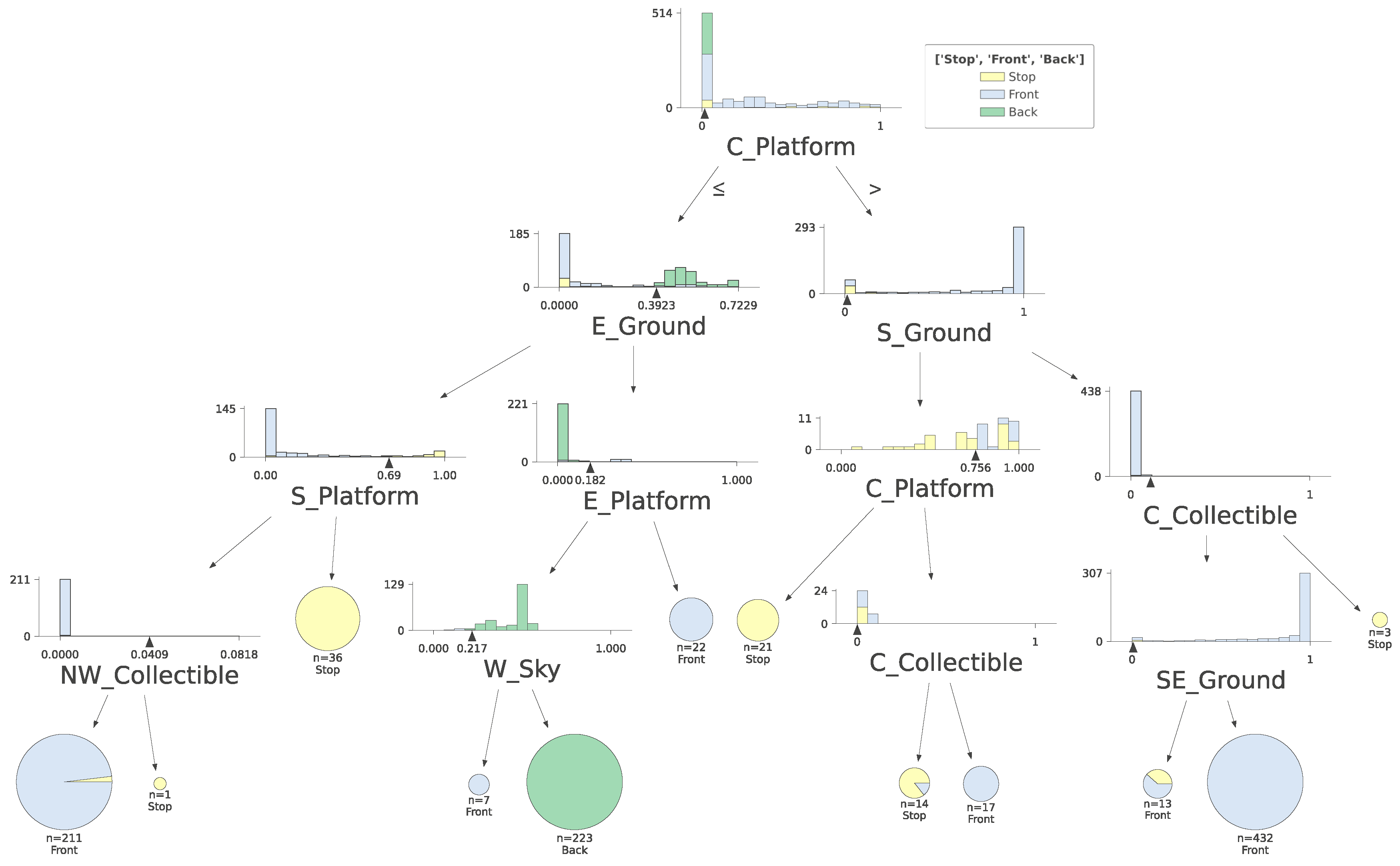
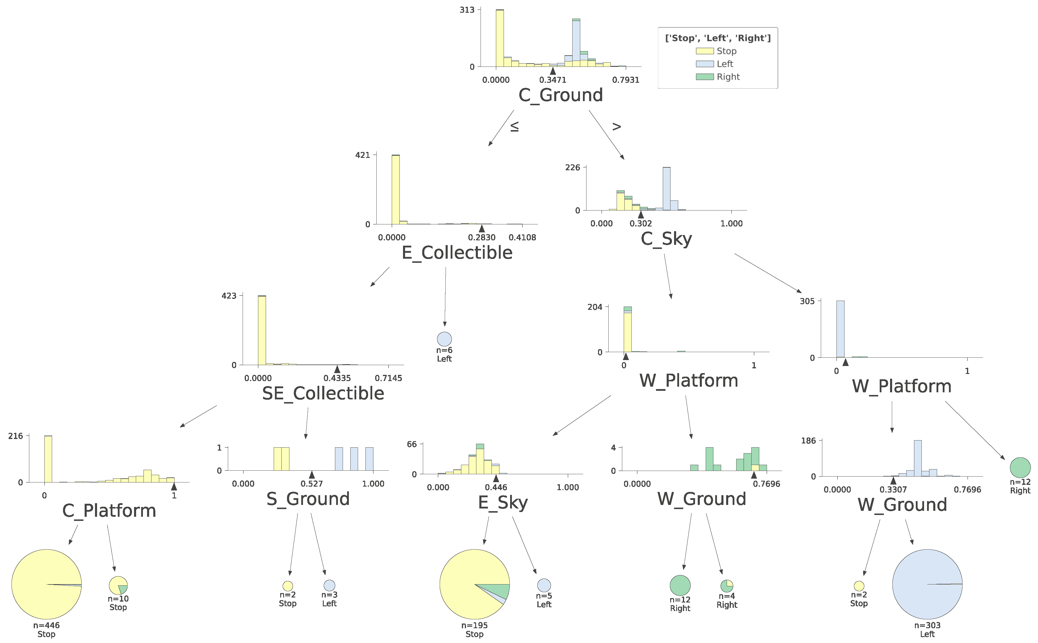
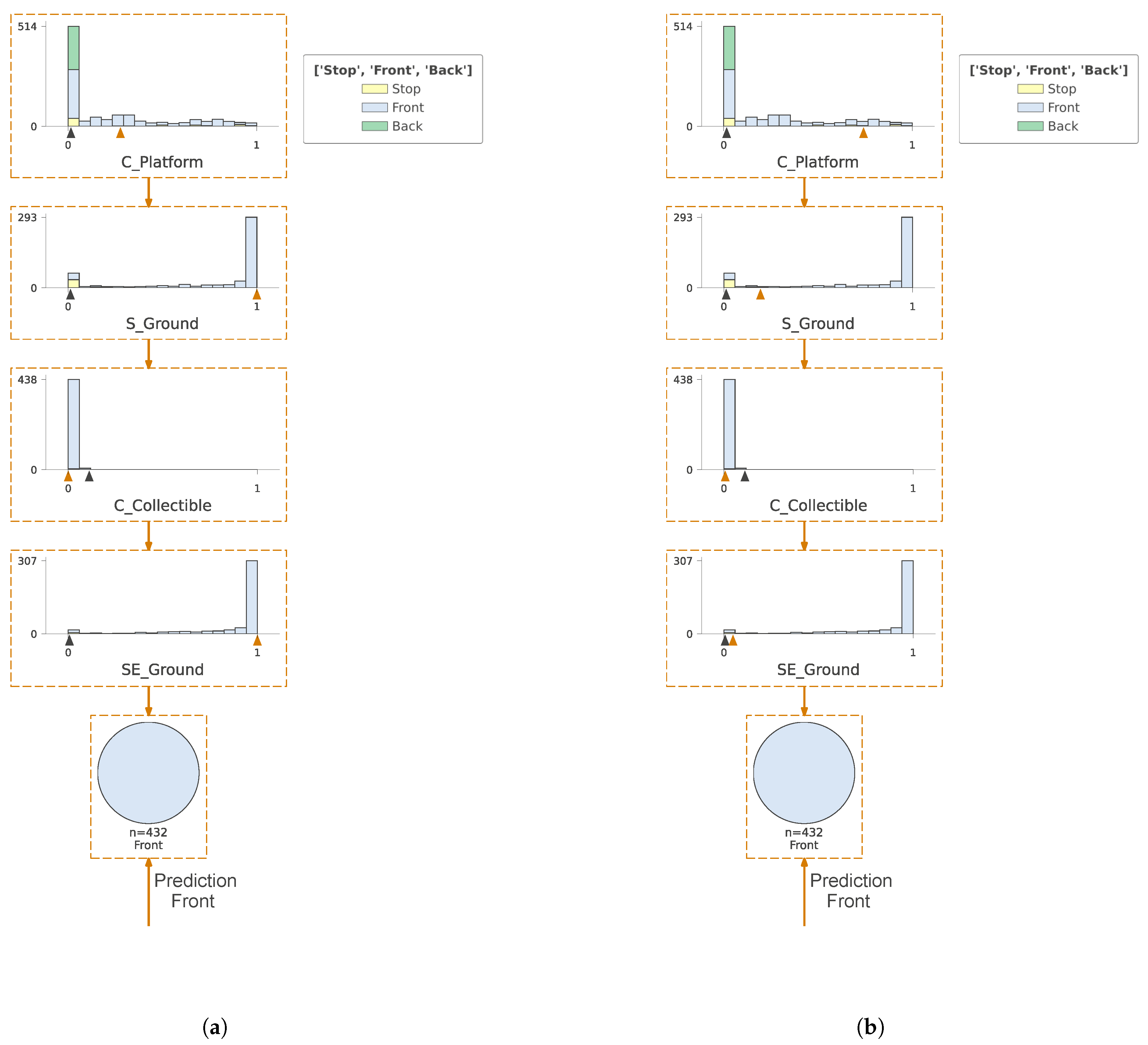
• model distillation (indirect inference): training of a simpler model (e.g., a decision tree) [46] whose task is to mimic the performance of a more complex RL agent on the assumption that a simpler model is more straightforward to interpret and can provide more comprehensible information about the agent’s decisions.

Detailed surveys on RL method explanation can be found in papers [47,48,49,50].

1.2. Novelty of This Paper

Based on the literature review from the above section, the topic of the explainability of machine learning models in reinforcement learning is actual and worth further investigation. Despite intensive research in this area, many open research problems exist, such as explaining the operation of training methods that use image data as input. In this work, we address the issues of the explainability of reinforcement learning-based machine learning agents trained with Proximal Policy Optimization (PPO) [51] that utilizes visual sensor data, which, to our knowledge, still needs to be sufficiently researched. We propose an algorithm that allows an effective and intuitive approximation of the PPO neural network. We also conduct several experiments to confirm our method’s effectiveness.

The rest of the paper is organized in the following way: in Section 2.1, Section 2.2, Section 2.3, Section 2.4 and Section 2.5, we introduce mathematical principles of Proximal Policy Optimization and GradCAM, which are used to introduce proposed explaining model presented in Section 2.3 and Section 2.4. In Section 2.6, we present the experiment settings used to prove the effectiveness of the proposed solution. Section 3 shows the experiments described in Section 2.6. Section 4 critically discusses the results showing the proposed method’s strengths and limitations. Final Section 5 summarizes the paper and indicates possible future research directions.

2. Materials and Methods

At the beginning of this section, we discuss a neural network (NN) of an agent trained with Proximal Policy Optimization (PPO) [52] with visual (image) input. Then, we revise a GradCAM method for image explanation. Later, we introduce a proposed method for explaining a PPO-generated NN with decision trees [53] trained with features generated by applying proxy geometry and semantic scene segmentation with GradCam weights.

2.1. The Neural Network of an Agent Trained with Proximal Policy Optimization with Visual (Image) Input

In Figure 1, we present an illustration of agent–environment interaction in reinforcement learning. In this machine learning scenario, agents can act in the environment and acquire observations. The goal of an agent is to maximize reward.

Applying the reinforcement learning model of the agent system based on the Proximal Policy Optimization algorithm [54] has become very popular in recent years. This algorithm approximates the value of the on-policy action–state pair function. We define the value of the On-Policy Action–Value Pair Function $Q^{\pi }(s,a)$ as the expected value of the cumulative reward function in case we start the calculation from state s, perform action a and always follow strategy $\pi$:

$$Q^{\pi }(s,a)=E_{\tau \sim \pi }R\left(\tau \right)\left|s_0=s,a_0=a\right.$$

(1)

We define the value of the Optimal Value Function $V^{*}\left(s\right)$ as the expected value of the cumulative reward function in case we start the calculation from state s and always follow the optimal strategy:

$$V^{*}\left(s\right)=\underset{\pi }{max}{E}_{\tau \sim \pi }R\left(\tau \right)\left|s_0=s\right.$$

(2)

We define the value of the Optimal Action–Value Function $Q^{*}(s,a)$ as the expected value of the cumulative reward function in case we start the calculation from state s, perform action a and always follow the optimal strategy:

$$Q^{*}(s,a)=\underset{\pi }{max}{E}_{\tau \sim \pi }R\left(\tau \right)\left|s_0=s,a_0=a\right.$$

(3)

Algorithms in the strategy optimization group define it as ${\pi }_{\varphi }\left(a\right|s)$. Optimization of $\varphi$ is performed directly by the gradient algorithm based on the gradient ascent with respect to $J\left({\pi }_{\theta }\right)$ (the expected value of strategy $\pi$) or its local approximation.

The practical implementation of PPO-trained agent control is defined in the form of a neural network (NN), which we call the brain of an agent, consisting of two parts: the feature extraction module and the decision module. Figure 2 presents two example agent brains. These two example agents make decisions based on image data encoded in three-dimensional tensors. Image data are processed by a convolutional neural network (or any other feature extractor), reshaped to match the size of decision layers, and then processed by classification layers to commit decisions on agents’ behavior. In Figure 2, the left network uses a “Simple” encoder that uses two convolutional layers, and the right uses a “Nature” network proposed in [35]. The rest of the NN is nearly identical in both cases. The convolutional network reported in [35] is an image features extractor for a fully connected neural network able to replace a human player in the decision-making process in 49 benchmark games. The “Simple” network is a smaller variation of the “Nature” approach. These two architectures are state-of-the-art brains for PPO-trained agents in the very popular ML agents library in the Unity virtual environment. For this reason, we decided to conduct our experiments on these two architectures. The action is performed with two fully connected layers with Sigmoid activation functions (the number of layers might vary depending on the problem). The final action of the agent is returned with several output layers (the number of outputs depends on the problem); in Figure 2, there are three output layers. In the case of classification tasks, there is often a Softmax layer following each output; it is removed here for clarity. As can be seen, there is also one additional input in both networks called “action_masks”, a special case of NN implementation for the ML Agents library in Unity. This input allows resetting selected network outputs.

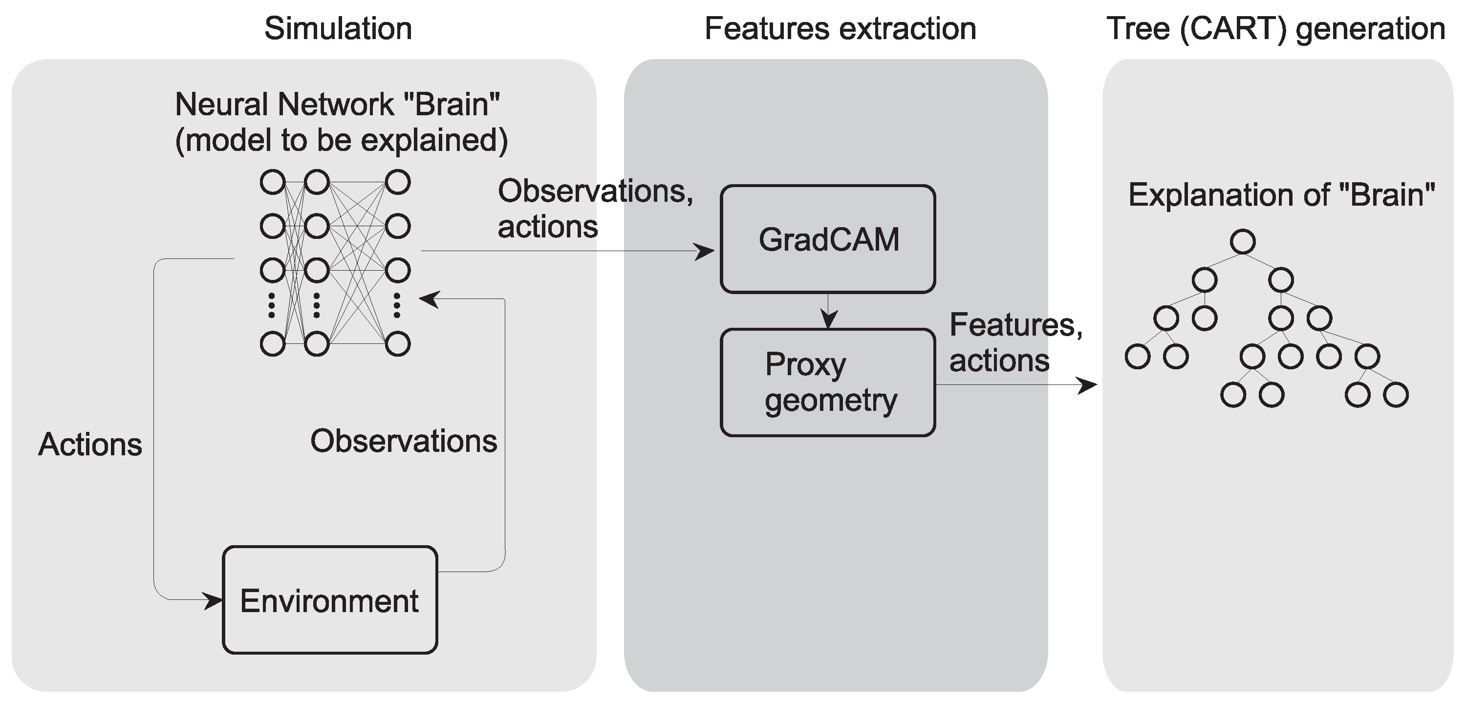
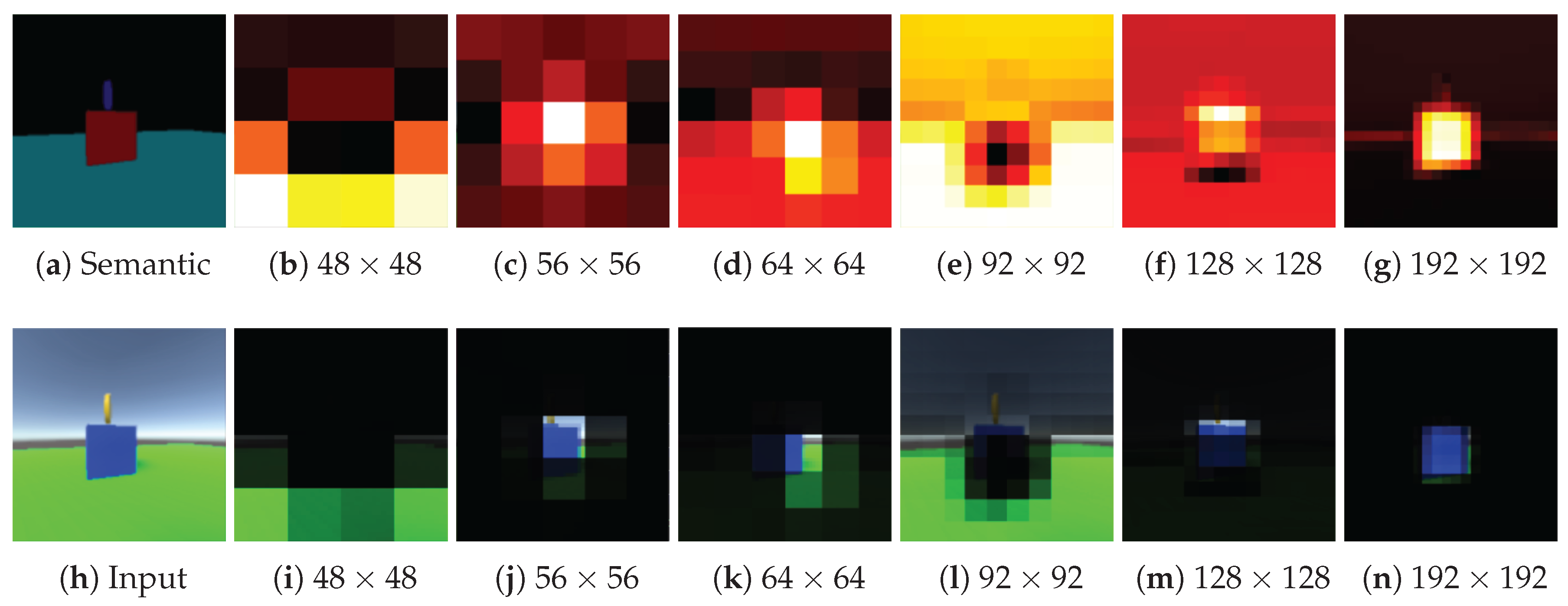
2.2. GradCAM for Image Processing Layer Explanation

GradCAM [33] is among the most popular algorithms for visually explaining convolutional neural networks. This is a gradient-based approach that is based on the assumption that the areas of the last convolutional layer of the network whose values vary the most as a result of stimulating the network with a signal representing an object belonging to that class have the most significant influence on the classification of an object into a particular class. In practice, GradCAM computes the average of the gradient values and uses them in linear combination with the output of the last convolutional layer. In the linear combination, only the sum’s non-negative components are considered. The resulting feature relevance map is often scaled to an interval of values [0, 1] and then interpolated and superimposed on the input image. This second step is because convolutional features retain spatial information about the input signal. After overlaying the relevance map, GradCAM marks the areas of the input image that are most significant for classification into a particular class. The algorithm can be written as follows: suppose we have an input image I that can be classified into C classes. Each class is represented by a separate output from the $y_c$ network. Suppose the last convolutional layer of the network consists of K filters; each filter returns a resultant image (feature set) with a resolution of $n\times m$. We calculate the weights $w_k^c$ for the given class c and the kth output of the last convolutional layer as follows:

$$w_k^c={\displaystyle \frac{{\sum }_{i=1}^n{\sum }_{j=1}^m\frac{\partial y^c}{\partial A_{i,j}^k}}{n·m}}$$

(4)

where $y^c$ is an output of the neural network that corresponds to classification of an input I to class c, $A_{i,j}^k$ is a feature with coordinates $(i,j)$ of the kth output of the last convolutional layer, $k\in [1,\dots ,K]$, $c\in [1,\dots ,C]$. Finally, the GradCAM map $M^c$ generated for class c is computed as follows:

$$M^c=Scal{e}_{[0,1]}\left(max(0,\sum _{k=1}^K{w}_k^c·A^k)\right)$$

(5)

where $Scal{e}_{[0,1]}$ scales input tensor values to range $[0,1]$ linearly.

GradCAM can be directly applied to convolutional neural networks where the last convolutional layer can be indicated. In particular, GradCAM can be applied to the example Simple and Nature feature extractors shown in Figure 2.

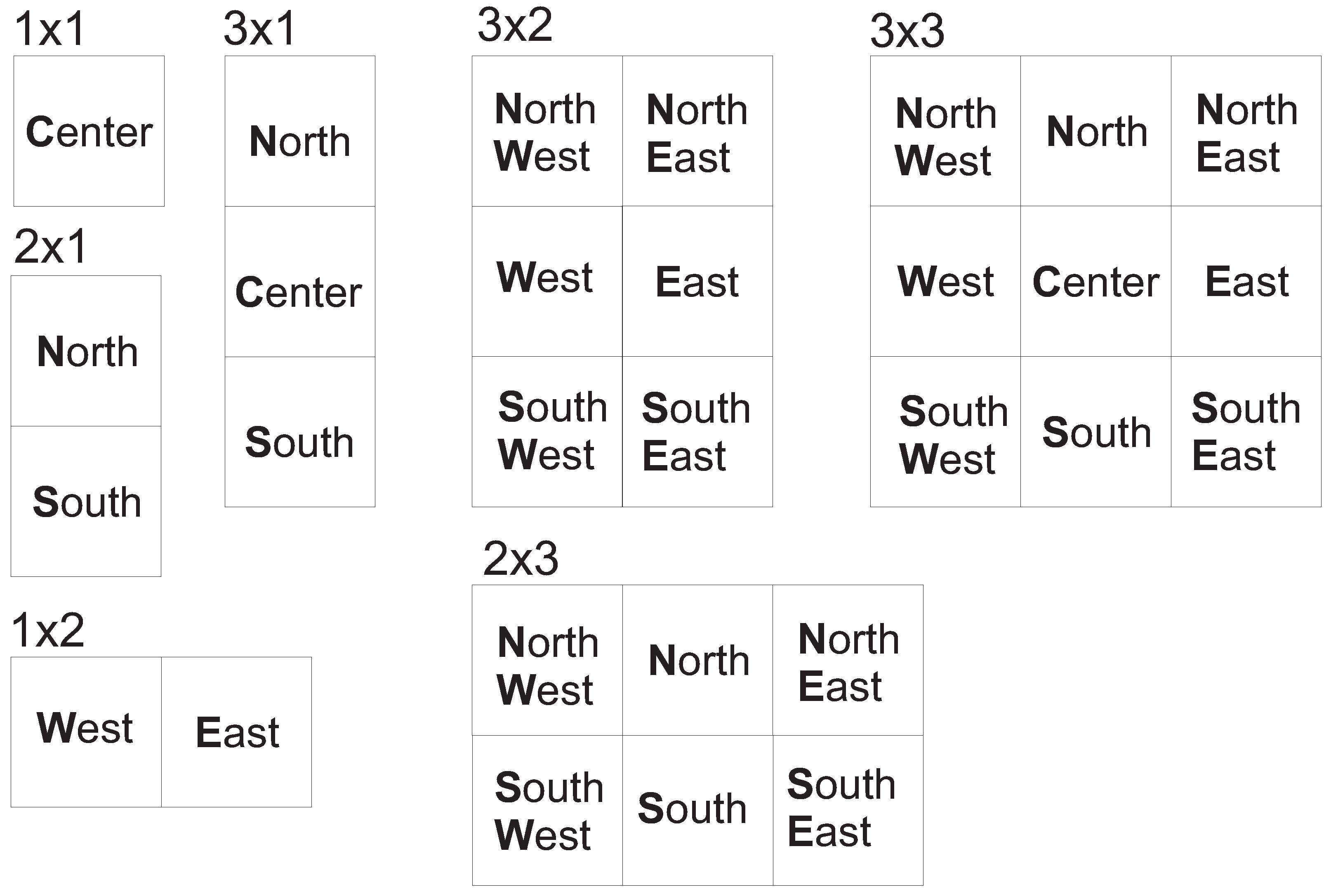
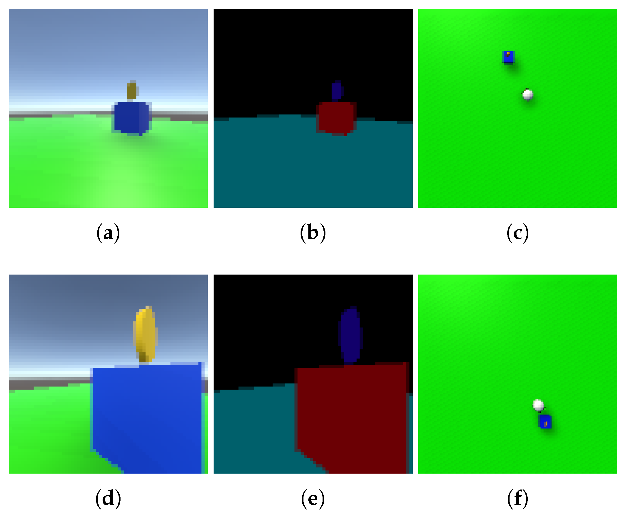
2.3. Decision Trees, Proxy Geometry and Semantic Scene Segmentation

An informative way to represent an algorithm is to describe it as a flowchart containing control instructions such as loops, conditional statements, etc. An alternative approach is to use a special case of the block diagram as what can be considered a decision tree. A representation of a deep model in the form of a decision tree can meet the requirements for an explanation for a black-box machine learning model because we can estimate its accuracy (how well an explanation predicts unseen data), fidelity (explanations ought to be close to the predictions of the explained) and comprehensibility (explanations should be understandable to humans) [53]. Using a decision tree to explain an algorithm that relies on visual data is more complex. Several factors influence this:

• Input image to the model, even if it is not high-resolution, for example, $48\times 48$ pixels, contains 2304 features. This is far too many to build an explanation of the model.
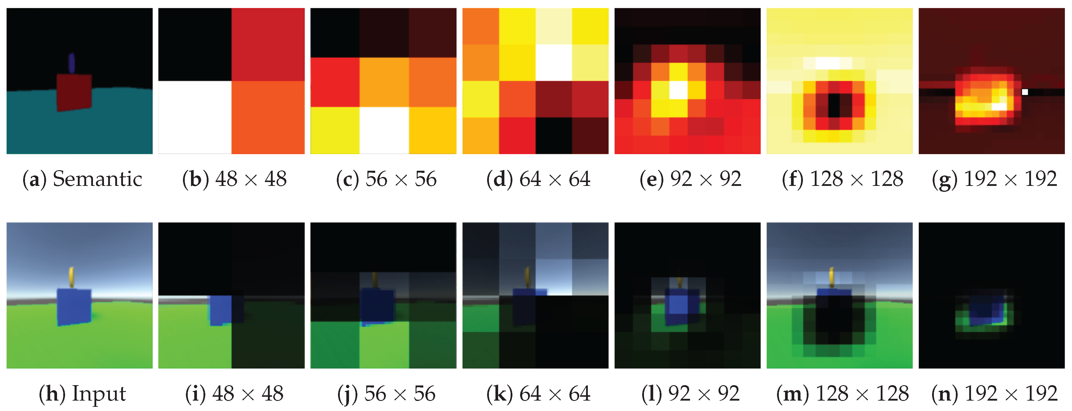
• Individual pixels are not a semantic interpretation of what is in the image. What is interpretable is their position relative to each other. The convolution layer, acting as a multi-cascade image filter, analyzes the textures and mutual position of graphic primitives in the image.

Therefore, to make the vision model explainable as a decision tree, it is necessary to reduce the number of features and replace visual information, which is based on colored pixels, with semantic information, which is based on types (classes) of objects located in specific areas of the input image.

The limitation of the number of features should be tuned so that the new set of features retains information about the spatial position of objects in the image and is easy to interpret for human cognitive interpretation. The labels of individual features should also be easy to identify. To meet all these requirements, we use a proxy geometry known for creating visual human–computer interfaces [55] based on dividing the space into up to $(3\times 3)$ parts whose names are based on geographic directions. Depending on the resolution of the $(n\times m)$ GradCAM map $M^c$, there may be several combinations of the set of proxy geometries, which we show in Figure 3. The type of proxy geometry is calculated according to Algorithm 1 by executing it for the values n and m, and the proxy region borders thus built are stored in variables $border{s}_n,border{s}_m$, respectively. The naming convention for the individual features that are in matrix F is as in Figure 3. This algorithm does not consider the size of the input image I but the resolution of $M^c$. This is because if $M^c$ has a relatively small resolution, after scaling it to the resolution of I and extracting features from it in the rest of the algorithm, interpolation of map values during resampling may result in the assignment of objects from different areas of $M^c$ to one proxy geometry area. If the resolution of $M^c$ is much smaller than the resolution of the image, this can result in an erroneous averaging of the excitation areas of $M^c$ into several adjacent proxy geometry areas.

The next important step is to extract the semantic information from the input image, in other words, segmenting the objects that make up the observed scene. This is an intuitive approach: to understand the operation of the decision-making process based on the image content, the user does not derive relevant information from the color values in the observed proxy geometry area but is rather interested in the types of objects that the algorithm observes. It is therefore necessary to provide a semantic segmentation of the observed scene to the explanatory algorithm. Another machine learning algorithm can be used for this, for example, [56,57,58,59], or if the algorithm is tested in a virtual environment, data can be obtained directly from it. Nowadays, reinforcement learning model evaluation in the virtual environment is a common and much cheaper approach than building a real-life prototype [60,61], so we can assume that it is possible to obtain semantic data directly from the virtual environment. In Figure 4, we show an example visualization of the virtual world as seen by an agent (first column) and a semantic segmentation of the objects visible in the scene (second column).

Algorithm 1: Generate proxy geometry

After creating the proxy geometry and performing segmentation, we can proceed with feature generation. The algorithm that generates features is shown in Algorithm 2. It involves performing GradCAM for an image I and then a weighted summation of the pixels that belong to each semantic object class within each proxy geometry segment. The weights are determined based on the GradCAM values after any additional correction is made by powering up with an exponent $(\alpha \ge 1$) and a threshold $t\in [0,1]$. The use of $(\alpha ,t)$ is intended to filter the GradCAM map from values characterized by a small network gradient. The higher the $\alpha$ value, the more the map values close to 0 are reduced, and map values equal to 1 remain unchanged. The weighted sums within each segment are scaled such that the sum for each class in the segment is divided by the weighted sum of the pixels in all classes in that segment. Following this approach, the proxy geometries within each segment are then scaled by dividing each feature by the weighted sum of all pixels in the segment. Ultimately, therefore, each feature has a value in the range of $[0,1]$, and the sums of feature values within a segment are 0 if for each pixel in that segment $M^c\left(I\right)$ is 0 or 1 otherwise. We name the individual features according to the name of the segment and the name of the semantic class to which the pixels in the segment belong. For example, suppose the proxy geometry is of size $(2\times 1)$ {North, South}, and there are three semantic classes {Class1, Class2, Class3}. The set defined in this way has $(2·3=6)$ features named {North_Class1, North_Class2, North_Class3, South_Class1, South_Class2, South_Class3}. In the case of proxy geometry of size $(3\times 2)$ {NorthWest, NorthEast, West, East, SouthWest, SouthEast}, and there are two semantic classes {Class1, Class2}, we have $(6\dot{2}=12)$ features named {NorthWest_Class1, NorthWest_Class2, NorthEast_Class1, NorthEast_Class2, West_Class1, West_Class2, East_Class1, East_Class2, SouthWest_Class1, SouthWest_Class2, SouthEast_Class1, SouthEast_Class2}.

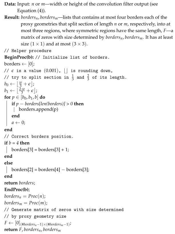
Algorithm 2: Generate image features using proxy geometry

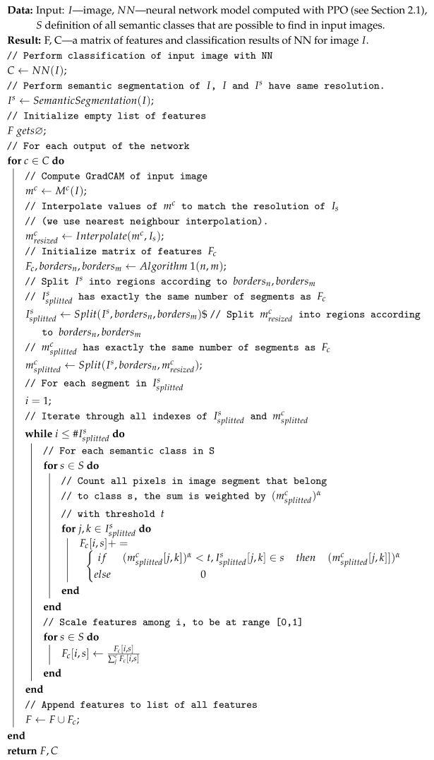
2.4. PPO Model Approximation with Decision Tree-Based Naive Method and with GradCam Weights

As presented in Section 2.3 as the result of applying Algorithms 1 and 2, we obtain a pair $F,C$, which is a set of features and classification results of the NN model. This information is sufficient to use them as a training dataset for the CART (Classification And Regression Tree) decision tree model to approximate the original NN [62]. In the case of the classification model, we use a Gini–Simpson index (Gini) for the splitting criterion. Gini impurity estimates the probability of incorrect labeling of a random sample element if classified randomly and independently according to the distribution of classes in the training dataset. CART performs locally optimal decisions at each split and minimizes the following loss function:

$$H\left(Q_j\right)=\sum _c^{\#C}{p}_j^c(1-p_j^c)$$

(6)

where $Q_j$ is data at node j and $p_j^c$ is the probability of correct assignment of all elements of class c to class c in dataset $Q_j$.

Decision trees generated by the CART algorithm are easy to analyze due to nicely explainable splitting criteria. We can also use them to track not only numbers but also particular instances of data samples that decide on certain tree splits. That information can be used during classification to justify the classifier’s decision. Summing up, the NNs in Section 2.1 are explained using an approximation CART model with features generated as presented in Section 2. If we look closely into Algorithm 2, we can notice that it might also be possible to generate the features set from training data using proxy geometry and semantic classification $I^s$ without GradCam map $M^c\left(I\right)$. This approach is called a Naive Method. The Naive Method has the same algorithm as Algorithm 2, but the GradCAM map is replaced by a matrix with the exact dimensions as GradCAM but filled with ones. Thanks to that, all pixels in the semantic image have the same weight and are of the same importance for further feature generation.

PPO-trained NNs can have more than one output. In most cases, this means that based on a specific input signal, an agent might perform more than one action simultaneously. In that case, each input–output relation has to be approximated by a separate decision tree. In Figure 5, we present a block diagram summarizing the proposed methodology.

2.5. Computational Complexity and Comparison with Other Methods

The computational complexity of the proposed algorithm depends on the number of decisions an agent performs during each step, which is equal to the number of outputs of brain network $\#C$, number of semantic classes (objects types) $\#S$, input image resolution $\#I$ and number of observations we acquired to generate CART $\#obs$. The complexity of GradCAM depends on the resolution of image I, $\#I$, and equals $O(\#I)$. Then, for each semantic class in S, we count all pixels in the image segment that belong to class $s\in S$. That operation has complexity $O(\#S·\#I)$. Suppose the proxy geometry has a size equal to 9, which is the highest possible value. Due to this, there are $9·\#S$ features. The computational complexity of creating CART is $O(9·\#S·\#obs·lo{g}_2(\#obs))\approx O(\#S·\#obslo{g}_2(\#obs))$ and we have to create a CART tree for each network output $\#C$. Finally, the computational complexity of our approach is $O(\#C·(\#I+\#S·\#I+\#S·\#obs·lo{g}_2(\#obs)))\approx O(\#C·\#S·(\#I+\#obs·lo{g}_2(\#obs)))$.

As can be seen, the computational complexity of our approach does not exceed the computational complexity of generating CART $\#C$ times, provided that $\#I\ll \#obs$; if $\#obs\ll \#I$, it becomes polynomial. This complexity allows a relatively fast generation of approximation of explained models.

Our approach utilizes decision tree formalism, which makes it similar to policy explanation approaches [38,39,40]. However, that method cannot be directly applied to visual data to produce explainable (understandable to the user) descriptions due to the high dimensionality of images. Similarly to visualization techniques, we also apply a GradCAM [43,44]; however, the explanation is not only based on visual feedback but also generates rules in the form of CART that govern the behavior of an agent. Our solution also uses a knowledge distillation approach [46] in which a black-box brain provides training data (feature-based knowledge) for its easy-to-interpreted approximation. To summarize, our method incorporates several elements from already established approaches and creates a single, easy-to-interpreted tree-based solution, thanks to which it can be applied in the domain of explaining the action of an agent collecting visual data, which none of the above methods can achieve individually.

2.6. Experiment Setting

To evaluate our approach, we performed experiments using a Unity Real-Time Development Platform (Unity) utilizing Unity Machine Learning Agents Toolkit (ML-Agents). The Agent’s task was to find a gold rotating cylinder (Collectible) positioned on a blue box (Platform). The Agent had to jump on the Platform to collect the Collectible. Collecting the Collectible under the time limit indicated the success of the training episode. Agent and Platform were modeled as rigid bodies that moved on a green floor (Ground). A simulation also included a blue sky (Sky). There were constraints on the time when the Agent must reach the target and the constraint on maximum distance from Collectible. When that distance was exceeded, the training episode ended in failure. The Agent could perform three actions, within which there were several mutually exclusive movements: backward, forward or no movement (Backward, Forward, Stop), turn left, right or no turn (Left, Right, Stop), jump or not to jump (Jump, Ground). The Agent collected RGB data using a visual sensor (camera). We considered six different camera resolutions: $(48\times 48)$, $(56\times 56)$, $(64\times 64)$, $(96\times 96)$, $(128\times 128)$, $(192\times 192)$ and two feature-generating network architectures: “Simple” and “Nature” (see Section 2.1). The network making decisions about Agent movement consisted of two layers of 16 neurons, each with a Sigmoid activation function. The networks we used can be seen in Figure 2 (they had an additional Softmax layer after each output). The problem of decision-making by the Agent was a classification process. We ran $6·2=12$ experiments involving training the Agent for the six camera resolutions and two convolutional NNs. For each of the 12 possible configurations, we generated decision trees explaining the Agent’s NN performance using Algorithm 1 and Algorithm 2 with the methodology presented in Section 2.4. We used both the Naive Method and GradCAM-based method with all combinations of $\alpha$ and t parameter values in ranges $\alpha =1,2,3,5$ and $t=0,0.1,0.2,0.3,0.4,0.5$. Details of the environment configuration needed to reproduce the experiment are in the source codes, which can be downloaded from https://github.com/browarsoftware/ppo_explanation [accessed on 9 October 2024].

3. Results

The proposed method for explaining reinforcement learning-based machine learning agents trained with Proximal Policy Optimization was evaluated on a PC computer with Intel i7 2.3 GHz, 32 GB RAM, GeForce RTX 3050 GPU running Windows 11 OS. We used Unity engine 2021.3.18f1 and Ml Agents 2.0.1 for machine learning. The framework for agent training was Python 3.9 with libraries Torch 2.2.2, Tensorboard 2.17.1, mlagents 0.30.0, mlagents-envs 0.30.0, gym 0.26.2. For model explanation, we used Python 3.10, tensorflow 2.8, keras 2.8, scikit-learn 1.5.2, onnx 1.14.1, onnx2kears 0.0.24 (https://github.com/gmalivenko/onnx2keras [accessed on 9 October 2024]). Ml Agents generate a network in Onnx format that has to be converted to the Keras NN model to enable numerical differentiation of the network graph.

We performed all 12 experiments described in Section 2.6. A total of $15·{10}^5$ episodes were enough for each evaluated NN model to obtain $100\%$ efficiency in solving the problem of acquiring a Collectible object by an Agent. The plot with Cumulative Reward value during PPO training is presented in Figure 6. The vertical axis presents the number of training steps, while the vertical axis presents the cumulative reward of an agent. After training the agents so that each configuration had $100\%$ efficiency, we generated recordings of 1000 consecutive images from that Agent’s visual sensor and the corresponding semantic segmentations for those images. We used these images and segmentations to generate explanations according to our proposed method and validation with the leave-one-out test. In other words, each CART tree was trained on 999 images and validated on one, and the validation process was repeated 1000 times for each tree. A detailed description of the experiment setup can be found in Section 2.6.

In Figure 7 and Figure 8, we present example GradCAM results for various Agent NNs differing with a resolution of the image sensor. All agents use a “Simple” convolutional features embedder. In (a), the semantic clustering of the input image (h) is presented. The first row presents the GradCAM color-coded map generated as the response of the NN for the input image (h). The second row shows the same GradCAM map but is imposed onto the input signal. The darker the region, the smaller the value on the map. The bright areas correspond to a value of one on the GradCAM map.

In Figure 9, Figure 10 and Figure 11, we present a CART explanation generated by the proposed GradCAM-based method for the Agent’s NN with $(64\times 64)$ input image signal, “Simple” convolutional feature embedder, and $(\alpha =1,t=0.3)$ parameters of Algorithm 2. Those trees explain the rules of front–back, left–right, and jumping motion, respectively. Instances of classes among certain features are presented in color-coded bars. The black arrow positioned under the horizontal axis indicates the splitting threshold.

Figure 4 in each row presents the triplet of the input image (view from the Agent’s camera), its semantic (object class-based) segmentation and visualization of the Agent’s position (represented by a white capsule shape) towards the blue platform (a bird-eye view of the scene). Figure 12, Figure 13 and Figure 14 present the decision process (predictions) of the CART tree generated by the proposed GradCAM-based method for Agent’s NN with $(64\times 64)$ input image signal, “Simple” convolutional feature embedder, $(\alpha =1,t=0.3)$ on images from Figure 4. The orange arrow under the horizontal axis indicates the actual feature value. These figures show an explanation of the decision-making process for a single-agent camera reading. They contain single tree paths from trees shown in Figure 9, Figure 10 and Figure 11.

In

Table 1. Results of the leave-one-out accuracy test of various configurations of the Agent’s NN explanation method presented in Section 2.4. Rows represent various parameter settings, and columns represent the resolution of the input image. All results are for “Simple” convolution feature extraction.

	$48\times 48$	$56\times 56$	$64\times 64$	$96\times 96$	$128\times 128$	$192\times 192$
Naive	0.945	0.961	0.963	0.962	0.967	0.932
$\mathbf{\alpha }$ = 1; t = 0	0.959	0.977	0.976	0.968	0.962	0.941
$\mathbf{\alpha }$ = 1; t = 0.1	0.953	0.982	0.976	0.969	0.968	0.944
$\mathbf{\alpha }$ = 1; t = 0.2	0.955	0.984	0.976	0.967	0.970	0.943
$\mathbf{\alpha }$ = 1; t = 0.3	0.949	0.982	0.982	0.961	0.955	0.93
$\mathbf{\alpha }$ = 1; t = 0.4	0.942	0.981	0.976	0.959	0.948	0.93
$\mathbf{\alpha }$ = 1; t = 0.5	0.944	0.977	0.976	0.966	0.946	0.935
$\mathbf{\alpha }$ = 2; t = 0	0.944	0.978	0.976	0.967	0.966	0.945
$\mathbf{\alpha }$ = 2; t = 0.1	0.946	0.98	0.976	0.964	0.958	0.941
$\mathbf{\alpha }$ = 2; t = 0.2	0.952	0.982	0.974	0.96	0.937	0.938
$\mathbf{\alpha }$ = 2; t = 0.3	0.944	0.969	0.977	0.954	0.935	0.929
$\mathbf{\alpha }$ = 2; t = 0.4	0.931	0.965	0.972	0.941	0.943	0.919
$\mathbf{\alpha }$ = 2; t = 0.5	0.937	0.971	0.962	0.942	0.928	0.918
$\mathbf{\alpha }$ = 3; t = 0	0.947	0.975	0.974	0.973	0.96	0.945
$\mathbf{\alpha }$ = 3; t = 0.1	0.953	0.984	0.973	0.961	0.945	0.931
$\mathbf{\alpha }$ = 3; t = 0.2	0.941	0.968	0.972	0.95	0.941	0.929
$\mathbf{\alpha }$ = 3; t = 0.3	0.935	0.968	0.968	0.936	0.936	0.913
$\mathbf{\alpha }$ = 3; t = 0.4	0.934	0.97	0.955	0.938	0.922	0.917
$\mathbf{\alpha }$ = 3; t = 0.5	0.927	0.97	0.935	0.911	0.918	0.901
$\mathbf{\alpha }$ = 5; t = 0	0.953	0.971	0.973	0.968	0.951	0.944
$\mathbf{\alpha }$ = 5; t = 0.1	0.934	0.968	0.97	0.941	0.94	0.922
$\mathbf{\alpha }$ = 5; t = 0.2	0.934	0.971	0.96	0.935	0.928	0.917
$\mathbf{\alpha }$ = 5; t = 0.3	0.929	0.968	0.948	0.916	0.922	0.901
$\mathbf{\alpha }$ = 5; t = 0.4	0.914	0.966	0.928	0.9	0.911	0.9
$\mathbf{\alpha }$ = 5; t = 0.5	0.896	0.959	0.901	0.846	0.913	0.891

and

Table 2. Results of the leave-one-out accuracy test of various configurations of the Agent’s NN explanation method presented in Section 2.4. Rows represent various parameter settings, and columns represent the resolution of the input image. All results are for “Nature” convolution feature extraction.

	$48\times 48$	$56\times 56$	$64\times 64$	$96\times 96$	$128\times 128$	$192\times 192$
Naive	0.919	0.953	0.944	0.911	0.961	0.956
$\mathbf{\alpha }$ = 1; t = 0	0.911	0.963	0.953	0.921	0.968	0.967
$\mathbf{\alpha }$ = 1; t = 0.1	0.917	0.966	0.961	0.926	0.965	0.962
$\mathbf{\alpha }$ = 1; t = 0.2	0.922	0.97	0.95	0.919	0.967	0.966
$\mathbf{\alpha }$ = 1; t = 0.3	0.914	0.97	0.953	0.908	0.964	0.964
$\mathbf{\alpha }$ = 1; t = 0.4	0.917	0.972	0.95	0.893	0.963	0.961
$\mathbf{\alpha }$ = 1; t = 0.5	0.915	0.962	0.956	0.874	0.957	0.954
$\mathbf{\alpha }$ = 2; t = 0	0.911	0.962	0.949	0.921	0.968	0.963
$\mathbf{\alpha }$ = 2; t = 0.1	0.918	0.973	0.957	0.912	0.961	0.963
$\mathbf{\alpha }$ = 2; t = 0.2	0.913	0.972	0.955	0.876	0.959	0.951
$\mathbf{\alpha }$ = 2; t = 0.3	0.92	0.965	0.946	0.874	0.951	0.954
$\mathbf{\alpha }$ = 2; t = 0.4	0.912	0.961	0.939	0.872	0.955	0.952
$\mathbf{\alpha }$ = 2; t = 0.5	0.918	0.934	0.937	0.863	0.947	0.949
$\mathbf{\alpha }$ = 3; t = 0	0.911	0.963	0.957	0.915	0.96	0.966
$\mathbf{\alpha }$ = 3; t = 0.1	0.911	0.97	0.953	0.878	0.959	0.953
$\mathbf{\alpha }$ = 3; t = 0.2	0.919	0.963	0.947	0.874	0.958	0.952
$\mathbf{\alpha }$ = 3; t = 0.3	0.917	0.957	0.937	0.863	0.948	0.949
$\mathbf{\alpha }$ = 3; t = 0.4	0.913	0.907	0.935	0.858	0.947	0.95
$\mathbf{\alpha }$ = 3; t = 0.5	0.913	0.922	0.933	0.844	0.939	0.942
$\mathbf{\alpha }$ = 5; t = 0	0.911	0.966	0.947	0.911	0.961	0.962
$\mathbf{\alpha }$ = 5; t = 0.1	0.914	0.964	0.943	0.869	0.953	0.948
$\mathbf{\alpha }$ = 5; t = 0.2	0.917	0.907	0.937	0.864	0.945	0.945
$\mathbf{\alpha }$ = 5; t = 0.3	0.914	0.921	0.935	0.847	0.937	0.947
$\mathbf{\alpha }$ = 5; t = 0.4	0.91	0.925	0.928	0.834	0.938	0.944
$\mathbf{\alpha }$ = 5; t = 0.5	0.905	0.926	0.935	0.819	0.931	0.935

, we present the results of statistical cross-validation analysis of our proposed method; best results are marked bold. We utilized the leave-one-out accuracy test of various configurations of the Agent’s NN explanation method presented in Section 2.4. Rows represent various parameter settings, and columns represent the resolution of the input image. Results are averaged values of all correct classifications of three possible agent actions (motion, rotation, jumping) over all possible decisions, which means the following:

$$ACC={\displaystyle \frac{P_{fb}+P_{lr}+P_j}{P_{fb}+N_{fb}+P_{lr}+N_{lr}+P_j+N_j}}$$

(7)

where $P_{fb}$$P_{lr}$$P_j$ are positive decisions (true positive + true negative) and $N_{fb}$$N_{lr}$$N_j$ are negative decisions (false positive + false negative) for forward–backward, left–right and jump decisions appropriately.

4. Discussion

As can be seen in Figure 6, all tested configurations of NNs trained with the PPO algorithm established $100\%$ effectiveness in solving the problem described in Section 2.6 after no more than $15·{10}^5$ episodes. For an observer who visually compares individual Agents’ actions, they behaved similarly in a virtual environment. At first, they made rotational movements until they did not find the Platform/Collectible object. They then moved toward it by jumping at the right moment, which allowed them to reach the Collectible object. However, each of these networks worked in a slightly different way. An important factor was that we used two feature extractors, “Simple” and “Nature”, which differed in the number of layers and the resolution of the last convolution layer. Also, the data coming from the input vision sensor varied significantly in resolution, from $(64\times 64)$ up to $(192\times 192)$. Thus, it was natural that the feature image extractor that provided different input data determined the inference by the following fully connected neural layers with sigmoid activation functions (see Figure 2). Example performance visualizations of convolution neural with various input image resolution networks processed by semantic segmentation and GradCam for the same input image can be seen in Figure 7 and Figure 8. Aware of a certain simplification, we call the area of the GradCAM map where the averaged gradient obtained the most significant value in this discussion the area observed by the Agent. In some cases, such an observable area was those portions of the map where the entire Platform or Collectible the Agent was aiming at was located. This situation happened in Figure 7c,g and Figure 8e. However, this was not the general rule. Sometimes the observed area included only a portion of the target, for example, in Figure 7f and Figure 8g, or the target and a portion of its surroundings, as in Figure 7d,e and Figure 8b–d,f or did not observe the area at all and observed only its surroundings like in Figure 7b. By GradCAM’s assumption, these areas were the most influential in separating images into the different classes of activity performed by the Agent.

Based on the results in Table 1 and Table 2, we can conclude that our proposed method allowed an efficient approximation of the decision made by the neural network. For the Naive Method, the accuracy of approximation was in the range of 0.932 (for a resolution of $(192\times 192)$) to 0.967 (for a resolution of $(128\times 128)$) for the “Simple” convolutional embedder and 0.911 (for a resolution of $(96\times 96)$) to 0.961 (for a resolution of $(128\times 128)$) for the “Natural” convolutional embedder. The use of GradCAM-based feature extraction allowed further improvement of NN approximation results. The GradCAM-based method had the best accuracy of approximation in the range of 0.945 (for a resolution of $(192\times 192)$) to 0.984 (for a resolution of $(56\times 56)$) for the “Simple” convolutional embedder and 0.922 (for a resolution of $(48\times 48)$) to 0.968 (for a resolution of $(128\times 128)$) for the “Natural” convolutional embedder. The use of GradCAM resulted in an improvement in NN approximation relative to the Naive method of about 0.01 to 0.02. Most often, our method had the highest approximation values for $\alpha =1$ and a low value of $t\in 0.1,0.2,0.3$. This means that to achieve good approximation, there is no need for additional modulation or thresholding of $M^c$ map. Also, no relationship was observed between the resolution of the input signal and the accuracy of approximation.

The decision trees that were generated using the method described in Section 2.4 were relatively easy to interpret. In the case of the experiment described in Section 2.6, we obtained three trees for each parameter setting, examples of which can be seen in Figure 9, Figure 10 and Figure 11. They approximated the NN decision classifying forward–backward moving, left–right turning, and jumping, respectively. Example decision paths of these trees are shown in Figure 12, Figure 13 and Figure 14. The decision paths should be analyzed in conjunction with Figure 4, which shows the input image to the NN network. In Figure 12 for both images, the decision to move forward was made. As can be seen, such a decision was made when the Central part of proxy geometry was occupied by an object of class Platform, the South part of the geometry was occupied by an object of class Ground, there was a low number of pixels of Collectible class in the Center, and there were pixels of class Ground in the South-East. In other words, the Agent moved forward if there was Ground under its “legs” and a Platform and a Collectible in front of it. In Figure 13, in both cases, the decision was “Stop”, which means there was no turn in the left or right directions. As can be seen, the decision was based on the statistic that Agents did not turn if both to the left and right of the Agent there were not a sufficiently large number of pixels belonging to the Platform and Collectible classes. Figure 14 shows the situation when the Jump was not made (a) and when the Agent jumped (b). As can be seen, the Jump was not executed because in the South area, there were not enough pixels belonging to the Platform class, and in the South East direction, there were no pixels belonging to the Sky class, but there were pixels of the Ground class. As can be seen in tree (b), the Agent performed the Jump action when there was a Platform object and relatively few pixels of the Ground class in the South area, in the region very close to the Agent. The Agent decided to jump when it moved close enough to the Platform.

Plotting CARTs as they are in Figure 12, Figure 13 and Figure 14 where, in addition, we present histograms of the values of each feature in the training set, visualizes how often a given case occurred in the observed environment. The experiment showed that the rules generated by the CART tree were not only characterized by a high level of accuracy but were relatively easy for humans to interpret and led to intuitive conclusions.

We can safely say that the high value of the ACC is the most important indicator that signalizes the successful approximation of a black-box model with its explainable equivalent. The $\alpha$ and t parameters of the proposed method has to be tuned experimentally; however, experiments showed that those values should have rather low values. In our experiment, t did not exceed 2, while $\alpha$ did not exceed 0.2. That other aspect is the relation between the maximal depth of CART and the possibilities of interpreting and understanding the rules contained in this tree by humans. The process of understanding and interpretation is directly related to the individual abilities of each person to analyze this type of conditional systems, but for sure the deeper the tree, the less understandable it becomes.

While dealing with scenarios with multiple actions or decisions, the depth of the decision tree may increase, making rule interpretation more complex. This fact is an inevitable consequence of using a complex decision system in agent control. The more possible actions an agent can take and the more semantic object classes can be distinguished in the environment, the more complex the agent control algorithm and, consequently, the decision tree that describes it usually becomes. To simplify the interpretation process, the tree size can be limited by specifying its maximum depth and the minimum number of samples required to split an internal node. This is a trade-off between the accuracy of the model’s description using the decision tree and the complexity of the tree, understood as its depth. A Gini impurity may estimate the overall fitting of the CART on the leaves of a decision tree.

Our method was evaluated in low-resolution visual systems with the highest considered resolution equaled $(192\times 192)$. The range of considered resolutions was determined by two factors. The first is the memory limitations of the hardware: the higher the camera’s resolution, the larger the input layers of the network (see Figure 2). When camera resolution increases, it becomes necessary to reduce the batch during training, and network learning becomes longer. The second factor was the lack of the dependence of Cumulative Reward value during PPO from the camera’s resolution. As shown in Figure 6, the resolution did not have a decisive effect on agent performance—regardless of the camera resolution, each agent completed the task. The camera’s high resolution does not critically affect the complication of the obtained explanation using the CART tree. First, the resolution of the analyzed image is not directly the resolution of the input image, but rather the resolution of GradCAM, or the last convolution layer of the feature extractor. In the case of our experiments, for $(48\times 48)$ resolution, GradCam had a resolution of $(4\times 4)$, for $(56\times 56)$—$(5\times 5)$, for $(64\times 64)$—$(6\times 6)$, for $(96\times 96)$—$(10\times 10)$, for $(128\times 128)$—$(12\times 12)$ and for $(192\times 192)$—$(20\times 20)$, which is much smaller than the input resolution of the camera. In addition, the heuristics we assumed use a proxy geometry with a maximum resolution of $3\times 3$ (see Figure 3). In summary, if we consider the image transmitted from the camera, the most significant factor in terms of the complexity of the decision tree is the number of semantic classes visible in the image, an issue we discussed earlier in this section.

5. Conclusions

Our proposed method works well for scenarios where semantic clustering of the scene is possible. It is based on the solid theoretical foundation of the GradCAM and CART with additional proxy geometry heuristics. It excelled in the explanation process in a virtual simulation system based on video data with relatively low resolution. It performs very well in multimedia systems, such as computer games or simulations, with a clearly defined Agent’s goal and few semantic classes. It can be used to provide an in-depth analysis of NN action rules generated in the PPO process by decision tree approximation. The rules generated by the CART tree are not only characterized by a high level of accuracy but are relatively easy for humans to interpret and lead to intuitive conclusions.

Our proposed method also has some limitations. First, if an agent can perform many possible actions (for example, a dozen quantized rotation directions), this could increase the depth of the decision tree and the difficulty of rule interpretation. Also, many semantic classes could cause difficulties in interpreting the tree due to the increasing complexity of the rules. The method proposed in the paper was tested and validated in a specific virtual environment. It has to be remembered that in many scenarios, the virtual environment is a basic and only environment where vision-based reinforcement learning algorithms operate, for example, in medical applications such as landmark detection, object tracking, image registration [63] or in computer games [35]. The generalization ability of the proposed algorithm in complex real-world environments remains an open question; however, currently used virtual reality systems have high rendering quality, creating almost photorealistic and physics-accurate simulation environments. For this reason, it can be anticipated that the application of the currently popular virtual-to-real-world transfer learning paradigm, which involves training a system used in the real world based on virtual/synthetic data [64], may allow the application of our algorithm for non-virtual objects. The issue of applying the solution proposed in this work to real-world and especially robotics applications is a promising research topic worth pursuing. Another interesting issue is the possibility of completely replacing the deep learning model with an explainable equivalent. This would be useful when an explainable equivalent would have virtually identical performance to the neural network approach. In our case, this would also require creating a fast, real-time, lightweight, and mobile GradCAM algorithm implementation, which is a technological challenge at the moment.

References

1. Ding, W.; Abdel-Basset, M.; Hawash, H.; Ali, A.M. Explainability of artificial intelligence methods, applications and challenges: A comprehensive survey. Inf. Sci. 2022, 615, 238–292. [Google Scholar] [CrossRef]
2. Gilpin, L.H.; Bau, D.; Yuan, B.Z.; Bajwa, A.; Specter, M.; Kagal, L. Explaining explanations: An overview of interpretability of machine learning. In Proceedings of the 2018 IEEE 5th International Conference on Data Science and Advanced Analytics (DSAA), Turin, Italy, 1–3 October 2018; pp. 80–89. [Google Scholar]
3. Holzinger, A.; Saranti, A.; Molnar, C.; Biecek, P.; Samek, W. Explainable AI methods—A brief overview. In Proceedings of the International Workshop on Extending Explainable AI Beyond Deep Models and Classifiers; Springer: Berlin/Heidelberg, Germany, 2022; pp. 13–38. [Google Scholar]
4. Lin, Y.S.; Lee, W.C.; Celik, Z.B. What do you see? Evaluation of explainable artificial intelligence (XAI) interpretability through neural backdoors. In Proceedings of the 27th ACM SIGKDD Conference on Knowledge Discovery & Data Mining, Singapore, 14–18 August 2021; pp. 1027–1035. [Google Scholar]
5. Rong, Y.; Leemann, T.; Nguyen, T.T.; Fiedler, L.; Qian, P.; Unhelkar, V.; Seidel, T.; Kasneci, G.; Kasneci, E. Towards human-centered explainable ai: A survey of user studies for model explanations. IEEE Trans. Pattern Anal. Mach. Intell. 2023, 46, 2104–2122. [Google Scholar] [CrossRef] [PubMed]
6. McDermid, J.A.; Jia, Y.; Porter, Z.; Habli, I. Artificial intelligence explainability: The technical and ethical dimensions. Philos. Trans. R. Soc. A 2021, 379, 20200363. [Google Scholar] [CrossRef] [PubMed]
7. Spartalis, C.N.; Semertzidis, T.; Daras, P. Balancing XAI with Privacy and Security Considerations. In Proceedings of the European Symposium on Research in Computer Security, The Hague, The Netherlands, 25–29 September 2023; pp. 111–124. [Google Scholar]
8. Akhtar, M.A.K.; Kumar, M.; Nayyar, A. Privacy and Security Considerations in Explainable AI. In Towards Ethical and Socially Responsible Explainable AI: Challenges and Opportunities; Springer: Berlin/Heidelberg, Germany, 2024; pp. 193–226. [Google Scholar]
9. Linardatos, P.; Papastefanopoulos, V.; Kotsiantis, S. Explainable AI: A review of machine learning interpretability methods. Entropy 2020, 23, 18. [Google Scholar] [CrossRef]
10. Ghosh, A.; Kandasamy, D. Interpretable artificial intelligence: Why and when. Am. J. Roentgenol. 2020, 214, 1137–1138. [Google Scholar] [CrossRef]
11. Hastie, T.; Tibshirani, R.; Friedman, J.H.; Friedman, J.H. The Elements of Statistical Learning: Data Mining, Inference, and Prediction; Springer: Berlin/Heidelberg, Germany, 2009; Volume 2. [Google Scholar]
12. Marcinkevičs, R.; Vogt, J.E. Interpretable and explainable machine learning: A methods-centric overview with concrete examples. Wiley Interdiscip. Rev. Data Min. Knowl. Discov. 2023, 13, e1493. [Google Scholar] [CrossRef]
13. Rawal, A.; McCoy, J.; Rawat, D.B.; Sadler, B.M.; Amant, R.S. Recent advances in trustworthy explainable artificial intelligence: Status, challenges, and perspectives. IEEE Trans. Artif. Intell. 2021, 3, 852–866. [Google Scholar] [CrossRef]
14. Minh, D.; Wang, H.X.; Li, Y.F.; Nguyen, T.N. Explainable artificial intelligence: A comprehensive review. In Artificial Intelligence Review; Springer: Berlin/Heidelberg, Germany, 2022; pp. 1–66. [Google Scholar]
15. Speith, T. A review of taxonomies of explainable artificial intelligence (XAI) methods. In Proceedings of the 2022 ACM Conference on Fairness, Accountability, and Transparency, Seoul, Republic of Korea, 21–24 June 2022; pp. 2239–2250. [Google Scholar]
16. Dwivedi, R.; Dave, D.; Naik, H.; Singhal, S.; Omer, R.; Patel, P.; Qian, B.; Wen, Z.; Shah, T.; Morgan, G.; et al. Explainable AI (XAI): Core ideas, techniques, and solutions. ACM Comput. Surv. 2023, 55, 1–33. [Google Scholar] [CrossRef]
17. Gianfagna, L.; Di Cecco, A. Model-agnostic methods for XAI. In Explainable AI with Python; Springer: Berlin/Heidelberg, Germany, 2021; pp. 81–113. [Google Scholar]
18. Darias, J.M.; Díaz-Agudo, B.; Recio-Garcia, J.A. A Systematic Review on Model-agnostic XAI Libraries. In Proceedings of the ICCBR Workshops, Salamanca, Spain, 13–16 September 2021; pp. 28–39. [Google Scholar]
19. Saeed, W.; Omlin, C. Explainable AI (XAI): A systematic meta-survey of current challenges and future opportunities. Knowl.-Based Syst. 2023, 263, 110273. [Google Scholar] [CrossRef]
20. Abusitta, A.; Li, M.Q.; Fung, B.C. Survey on explainable ai: Techniques, challenges and open issues. Expert Syst. Appl. 2024, 255, 124710. [Google Scholar] [CrossRef]
21. Le, T.T.H.; Prihatno, A.T.; Oktian, Y.E.; Kang, H.; Kim, H. Exploring local explanation of practical industrial AI applications: A systematic literature review. Appl. Sci. 2023, 13, 5809. [Google Scholar] [CrossRef]
22. Aechtner, J.; Cabrera, L.; Katwal, D.; Onghena, P.; Valenzuela, D.P.; Wilbik, A. Comparing user perception of explanations developed with XAI methods. In Proceedings of the 2022 IEEE International Conference on Fuzzy Systems (FUZZ-IEEE), Padua, Italy, 18–23 July 2022; pp. 1–7. [Google Scholar]
23. Saleem, R.; Yuan, B.; Kurugollu, F.; Anjum, A.; Liu, L. Explaining deep neural networks: A survey on the global interpretation methods. Neurocomputing 2022, 513, 165–180. [Google Scholar] [CrossRef]
24. Ribeiro, M.T.; Singh, S.; Guestrin, C. “ Why should i trust you?” Explaining the predictions of any classifier. In Proceedings of the 22nd ACM SIGKDD International Conference on Knowledge Discovery and Data Mining, San Francisco, CA, USA, 13–17 August 2016; pp. 1135–1144. [Google Scholar]
25. Lundberg, S. A unified approach to interpreting model predictions. arXiv 2017, arXiv:1705.07874. [Google Scholar]
26. Ribeiro, M.T.; Singh, S.; Guestrin, C. Anchors: High-precision model-agnostic explanations. In Proceedings of the AAAI Conference on Artificial Intelligence, New Orleans, LO, USA, 2–7 February 2018; Volume 32. [Google Scholar]
27. Friedman, J.H. Greedy function approximation: A gradient boosting machine. Ann. Stat. 2001, 29, 1189–1232. [Google Scholar] [CrossRef]
28. Goldstein, A.; Kapelner, A.; Bleich, J.; Pitkin, E. Peeking inside the black box: Visualizing statistical learning with plots of individual conditional expectation. J. Comput. Graph. Stat. 2015, 24, 44–65. [Google Scholar] [CrossRef]
29. Breiman, L. Random forests. Mach. Learn. 2001, 45, 5–32. [Google Scholar] [CrossRef]
30. Freedman, D.A. Statistical Models: Theory and Practice; Cambridge University Press: Cambridge, UK, 2009. [Google Scholar]
31. Wachter, S.; Mittelstadt, B.; Russell, C. Counterfactual explanations without opening the black box: Automated decisions and the GDPR. Harv. JL Tech. 2017, 31, 841. [Google Scholar] [CrossRef]
32. Simonyan, K. Deep inside convolutional networks: Visualising image classification models and saliency maps. arXiv 2013, arXiv:1312.6034. [Google Scholar]
33. Selvaraju, R.R.; Cogswell, M.; Das, A.; Vedantam, R.; Parikh, D.; Batra, D. Grad-CAM: Visual Explanations From Deep Networks via Gradient-Based Localization. In Proceedings of the IEEE International Conference on Computer Vision (ICCV), Venice, Italy, 22–29 October 2017. [Google Scholar]
34. Sutton, R.S. Reinforcement learning: An introduction. In A Bradford Book; MIT Press: Cambridge, MA, USA, 2018. [Google Scholar]
35. Mnih, V.; Kavukcuoglu, K.; Silver, D.; Rusu, A.A.; Veness, J.; Bellemare, M.G.; Graves, A.; Riedmiller, M.; Fidjeland, A.K.; Ostrovski, G.; et al. Human-level control through deep reinforcement learning. Nature 2015, 518, 529–533. [Google Scholar] [CrossRef]
36. Tesauro, G. Td-gammon: A self-teaching backgammon program. In Applications of Neural Networks; Springer: Berlin/Heidelberg, Germany, 1995; pp. 267–285. [Google Scholar]
37. Silver, D.; Huang, A.; Maddison, C.J.; Guez, A.; Sifre, L.; Van Den Driessche, G.; Schrittwieser, J.; Antonoglou, I.; Panneershelvam, V.; Lanctot, M.; et al. Mastering the game of Go with deep neural networks and tree search. Nature 2016, 529, 484–489. [Google Scholar] [CrossRef]
38. Sutton, R.S.; McAllester, D.; Singh, S.; Mansour, Y. Policy gradient methods for reinforcement learning with function approximation. Adv. Neural Inf. Process. Syst. 1999, 12, 1057–1063. [Google Scholar]
39. Shah, H.; Gopal, M. Fuzzy decision tree function approximation in reinforcement learning. Int. J. Artif. Intell. Soft Comput. 2010, 2, 26–45. [Google Scholar] [CrossRef]
40. Silva, A.; Gombolay, M.; Killian, T.; Jimenez, I.; Son, S.H. Optimization methods for interpretable differentiable decision trees applied to reinforcement learning. In Proceedings of the International Conference on Artificial Intelligence and Statistics, PMLR, Online, 26–28 August 2020; pp. 1855–1865. [Google Scholar]
41. Wang, C.; Aouf, N. Explainable Deep Adversarial Reinforcement Learning Approach for Robust Autonomous Driving. IEEE Trans. Intell. Veh. 2024, 1–13. [Google Scholar] [CrossRef]
42. Shukla, I.; Dozier, H.R.; Henslee, A.C. Learning behavior of offline reinforcement learning agents. In Proceedings of the Artificial Intelligence and Machine Learning for Multi-Domain Operations Applications VI, National Harbor, MD, USA, 22–26 April 2024; Volume 13051, pp. 188–194. [Google Scholar]
43. He, L.; Nabil, A.; Song, B. Explainable deep reinforcement learning for UAV autonomous navigation. arXiv 2020, arXiv:2009.14551. [Google Scholar]
44. Sarkar, S.; Babu, A.R.; Mousavi, S.; Ghorbanpour, S.; Gundecha, V.; Guillen, A.; Luna, R.; Naug, A. Rl-cam: Visual explanations for convolutional networks using reinforcement learning. In Proceedings of the IEEE/CVF Conference on Computer Vision and Pattern Recognition, Vancouver, BC, Canada, 17–24 June 2023; pp. 3861–3869. [Google Scholar]
45. Metz, Y.; Bykovets, E.; Joos, L.; Keim, D.; El-Assady, M. Visitor: Visual interactive state sequence exploration for reinforcement learning. In Proceedings of the Computer Graphics Forum, Los Angeles, CA, USA, 6–10 August 2023; Wiley Online Library: Hoboken, NJ, USA, 2023; Volume 42, pp. 397–408. [Google Scholar]
46. Hatano, T.; Tsuneda, T.; Suzuki, Y.; Imade, K.; Shesimo, K.; Yamane, S. GBDT modeling of deep reinforcement learning agents using distillation. In Proceedings of the 2021 IEEE International Conference on Mechatronics (ICM), Kashiwa, Japan, 7–9 March 2021; pp. 1–6. [Google Scholar]
47. Hickling, T.; Zenati, A.; Aouf, N.; Spencer, P. Explainability in deep reinforcement learning: A review into current methods and applications. ACM Comput. Surv. 2023, 56, 1–35. [Google Scholar] [CrossRef]
48. Puiutta, E.; Veith, E.M. Explainable reinforcement learning: A survey. In Proceedings of the International Cross-Domain Conference for Machine Learning and Knowledge Extraction, Dublin, Ireland, 25–28 August 2020; pp. 77–95. [Google Scholar]
49. Wells, L.; Bednarz, T. Explainable ai and reinforcement learning—A systematic review of current approaches and trends. Front. Artif. Intell. 2021, 4, 550030. [Google Scholar] [CrossRef]
50. Milani, S.; Topin, N.; Veloso, M.; Fang, F. Explainable reinforcement learning: A survey and comparative review. ACM Comput. Surv. 2024, 56, 1–36. [Google Scholar] [CrossRef]
51. Williams, R.J. Simple statistical gradient-following algorithms for connectionist reinforcement learning. Mach. Learn. 1992, 8, 229–256. [Google Scholar] [CrossRef]
52. Feng, Q.; Xiao, G.; Liang, Y.; Zhang, H.; Yan, L.; Yi, X. Proximal Policy Optimization for Explainable Recommended Systems. In Proceedings of the 2022 4th International Conference on Data-driven Optimization of Complex Systems (DOCS), Chengdu, China, 28–30 October 2022; pp. 1–6. [Google Scholar] [CrossRef]
53. Blanco-Justicia, A.; Domingo-Ferrer, J. Machine Learning Explainability Through Comprehensible Decision Trees. In Proceedings of the Machine Learning and Knowledge Extraction, Canterbury, UK, 26–29 August 2019; Holzinger, A., Kieseberg, P., Tjoa, A.M., Weippl, E., Eds.; ACM: Cham, Switzerland, 2019; pp. 15–26. [Google Scholar]
54. Schulman, J.; Wolski, F.; Dhariwal, P.; Radford, A.; Klimov, O. Proximal policy optimization algorithms. arXiv 2017, arXiv:1707.06347. [Google Scholar]
55. Niu, Y.-F.; Gao, Y.; Zhang, Y.-T.; Xue, C.-Q.; Yang, L.-X. Improving eye–computer interaction interface design: Ergonomic investigations of the optimum target size and gaze-triggering dwell time. J. Eye Mov. Res. 2019, 12. [Google Scholar] [CrossRef]
56. Asgari Taghanaki, S.; Abhishek, K.; Cohen, J.P.; Cohen-Adad, J.; Hamarneh, G. Deep semantic segmentation of natural and medical images: A review. Artif. Intell. Rev. 2021, 54, 137–178. [Google Scholar] [CrossRef]
57. Liu, X.; Deng, Z.; Yang, Y. Recent progress in semantic image segmentation. Artif. Intell. Rev. 2019, 52, 1089–1106. [Google Scholar] [CrossRef]
58. Khan, M.Z.; Gajendran, M.K.; Lee, Y.; Khan, M.A. Deep neural architectures for medical image semantic segmentation. IEEE Access 2021, 9, 83002–83024. [Google Scholar] [CrossRef]
59. Hachaj, T.; Piekarczyk, M. High-Level Hessian-Based Image Processing with the Frangi Neuron. Electronics 2023, 12, 4159. [Google Scholar] [CrossRef]
60. Sankar, K.; Pooransingh, A.; Ramroop, S. Synthetic Data Generation: An Evaluation of the Saving Images Pipeline in Unity. In Proceedings of the 2023 Congress in Computer Science, Computer Engineering, & Applied Computing (CSCE), Las Vegas, NV, USA, 24–27 July 2023; pp. 2009–2013. [Google Scholar] [CrossRef]
61. Tremblay, J.; Prakash, A.; Acuna, D.; Brophy, M.; Jampani, V.; Anil, C.; To, T.; Cameracci, E.; Boochoon, S.; Birchfield, S. Training deep networks with synthetic data: Bridging the reality gap by domain randomization. In Proceedings of the IEEE Conference on Computer Vision and Pattern Recognition Workshops, Salt Lake City, UT, USA, 18–22 June 2018; pp. 969–977. [Google Scholar]
62. Breiman, L. Classification and Regression Trees; Routledge: Oxfordshire, UK, 2017. [Google Scholar] [CrossRef]
63. Le, N.; Rathour, V.S.; Yamazaki, K.; Luu, K.; Savvides, M. Deep reinforcement learning in computer vision: A comprehensive survey. Artif. Intell. Rev. 2022, 59, 2733–2819. [Google Scholar] [CrossRef]
64. Ranaweera, M.; Mahmoud, Q.H. Virtual to Real-World Transfer Learning: A Systematic Review. Electronics 2021, 10, 1491. [Google Scholar] [CrossRef]
Figure 1. Illustration of agent–environment interaction in reinforcement learning.
Applsci 15 00538 g001
Figure 2. This figure presents two example agent brains trained with PPO consisting of convolutional image feature extractor and classification layers constructed by two 16-neuron layers. The names of the individual network elements are derived from the notation according to the ONNX data exchange standard (Open Neural Network Exchange, https://onnx.ai/onnx/ [accessed on 9 October 2024]). Gemm is matrix multiplication, Mul is element-wise multiplication, and Slice produces a slice of the input tensor along axes. Visualization was performed using Onnx-modifier software https://github.com/ZhangGe6/onnx-modifier [accessed on 9 October 2024]. (a) Agent’s NN with “Simple” convolutional feature extractor. (b) Agent’s NN with “Nature” convolutional feature extractor [35].
Applsci 15 00538 g002
Figure 3. Proxy geometry we used in proposed method.
Applsci 15 00538 g003
Figure 4. In this Figure, in each row, we present the triplet of the input image corresponding to semantic segmentation and visualization of the Agent’s position (white capsule shape) towards the blue platform. (a) Input image. (b) Semantic segmentation of the input image. (c) Bird-eye view of the scene. (d) Input image. (e) Semantic segmentation of the input image. (f) Bird-eye view of the scene.
Applsci 15 00538 g004
Figure 5. A block diagram summarizing the proposed methodology. At first, during the simulation, we gather observations and actions of the agent. Then, with the help of GradCAM and proxy geometry (see Algorithm 1), features are generated (see Algorithm 2). Those features and the agent’s actions are used to create an approximation of the neural network brain of an agent in the form of a decision tree (CART).
Applsci 15 00538 g005
Figure 6. The plot of Cumulative Reward value during PPO training steps (episodes).
Applsci 15 00538 g006
Figure 7. Example GradCAM results for various Agent NNs differing with a resolution of the image sensor. All agents use a “Simple” convolutional features embedder. (a) The semantic clustering of the input image (h). The first row presents the GradCAM color-coded map generated as the response of NN for input image (h). The second row shows the same GradCAM map but is imposed onto the input signal. The darker the region, the smaller the value on the map. The bright areas correspond to a value of 1 on the GradCAM map.
Applsci 15 00538 g007
Figure 8. Example GradCAM results for various Agent NNs differing with a resolution of the image sensor. All agents use a “Simple” convolutional features embedder. (a) Semantic clustering of the input image (h). The first row presents the GradCAM color-coded map generated as the response of NN for input image (h). The second row shows the same GradCAM map but is imposed onto the input signal. The darker the region, the smaller the value on the map. The bright areas correspond to a value of 1 on the GradCAM map.
Applsci 15 00538 g008
Figure 9. CART explanation generated by the proposed GradCAM-based method for Agent’s NN with ( 64 × 64 ) input image signal, “Simple” convolutional feature embedder and ( α = 1 , t = 0.3 ) parameters of Algorithm 2. This particular tree explains the rules of forward–backward motion. The size of the tree is limited to maximal depth of 4. Instances of classes among certain features are presented in color-coded bars. The black arrow positioned under the horizontal axis indicates the splitting threshold.
Applsci 15 00538 g009
Figure 10. CART explanation generated by the proposed GradCAM-based method for the Agent’s NN with ( 64 × 64 ) input image signal, “Simple” convolutional feature embedder and ( α = 1 , t = 0.3 ) parameters of Algorithm 2. This particular tree explains the rules of left–right motion. The size of the tree is limited to maximal depth of 4. Instances of classes among certain features are presented in color-coded bars. The black arrow positioned under the horizontal axis indicates the splitting threshold.
Applsci 15 00538 g010
Figure 11. CART explanation generated by the proposed GradCAM-based method for Agent’s NN with 64 × 64 input image signal, “Simple” convolutional feature embedder and ( α = 1 , t = 0.3 ) parameters of Algorithm 2. This particular tree explains the rules of jump motion. Instances of classes among certain features are presented in color-coded bars. The black arrow positioned under the horizontal axis indicates the splitting threshold.
Applsci 15 00538 g011
Figure 12. This Figure presents the decision process (predictions) of the CART tree generated by the proposed GradCAM-based method for Agent’s NN with ( 64 × 64 ) input image signal, “Simple” convolutional features embedder, ( α = 1 , t = 0.3 ) on images from Figure 4. The orange arrow under the horizontal axis indicates the actual feature value. This Figure shows an explanation of the decision-making process for a single agent camera reading. It contains a single tree path from the tree shown in Figure 9. (a) Prediction for input image from Figure 4a. (b) Prediction for input image from Figure 4d.
Applsci 15 00538 g012
Figure 13. This Figure presents the decision process (predictions) of the CART tree generated by the proposed GradCAM-based method for the Agent’s NN with ( 64 × 64 ) input image signal, “Simple” convolutional features embedder, ( α = 1 , t = 0.3 ) on images from Figure 4. The orange arrow under the horizontal axis indicates the actual feature value. This Figure shows an explanation of the decision-making process for a single Agent camera reading. It contains a single tree path from the tree shown in Figure 10. (a) Prediction for input image from Figure 4a. (b) Prediction for input image from Figure 4d.
Applsci 15 00538 g013
Figure 14. This Figure presents the decision process (predictions) of the CART tree generated by the proposed GradCAM-based method for the Agent’s NN with ( 64 × 64 ) input image signal, “Simple” convolutional features embedder, ( α = 1 , t = 0.3 ) on images from Figure 4. The orange arrow under the horizontal axis indicates the actual feature value. This Figure shows an explanation of the decision-making process for a single Agent camera reading. It contains a single tree path from the tree shown in Figure 11. (a) Prediction for input image from Figure 4a. (b) Prediction for input image from Figure 4d.
Applsci 15 00538 g014