Article

Inversion of Mechanical Parameters of Tunnel Surrounding Rock Based on Improved GWO-BP Neural Network

1
College of Civil Engineering, Hunan University of Science and Technology, Xiangtan 411201, China
2
Hunan Province Key Laboratory of Geotechnical Engineering Stability Control and Health Monitoring, Hunan University of Science and Technology, Xiangtan 411201, China
*
Author to whom correspondence should be addressed.
Appl. Sci. 2025, 15(2), 537; https://doi.org/10.3390/app15020537
Submission received: 17 October 2024 / Revised: 1 January 2025 / Accepted: 3 January 2025 / Published: 8 January 2025

Abstract

:
Accurately determining the mechanical parameters of surrounding rock in tunnel design and construction presents a significant challenge due to the complexity of the environment. This study proposes a novel approach for inverting these parameters using an advanced optimization method, the Improved Grey Wolf Optimization (IGWO), integrated with a BP neural network (IGWO-BP). Key enhancements such as cubic chaotic mapping, refraction backward learning, nonlinear convergence factors, and updated position formulas were applied to improve the algorithm’s search efficiency. By optimizing the neural network’s weights and biases, a precise relationship between rock mechanics and displacement was established. The method was validated through a case study of the Lianhua Tunnel (YK37 + 330 section), utilizing field data of crown settlement and peripheral displacement. The approach accurately predicted mechanical parameters, with relative errors below 5.02% for crown settlement and 4.15% for peripheral displacement. These results demonstrate the reliability and practical applicability of the proposed technique for tunnel engineering.

1. Introduction

The rapid advancements in computer technology have substantially bolstered both the theoretical foundation and practical applications of numerical analysis in geotechnical engineering. Despite the notable precision of contemporary numerical simulation models, the task of accurately identifying the requisite rock mechanics parameters continues to pose a considerable challenge. This difficulty primarily stems from several factors: the inherent complexity of underground structures, the unpredictability of geological conditions, the significant impact of scale effects in rock masses, and constraints in sample collection [1,2,3]. Consequently, accurately ascertaining the necessary rock mechanics parameters for these models has become a paramount challenge, central to the objectives of ongoing research.
To address this challenge, the back-analysis methodology was developed to accurately determine rock mechanics parameters, emerging as a trusted technique for pinpointing simulation parameters. Initiated in the 1970s, the technique of dynamic displacement back-analysis has achieved global recognition. Researchers utilize displacement data, monitored throughout the construction process, to inversely deduce the rock mass’s physical and mechanical characteristics and its constitutive model, contributing significantly to the field’s body of research [4,5,6,7,8,9]. Feng et al. [10] proposed the innovative Evolutionary Neural Network, combining artificial neural networks with Genetic Algorithms, demonstrating its effectiveness in back-analyzing elasticity problems. By merging Genetic Programming (GP) with numerical modeling, Ravandi et al. [11] created a database from simple, measurable parameters through backward analysis, accurately estimating the deformation modulus of rock masses and showcasing the computational program’s efficiency and precision. Miro et al. [12] developed a finite element model for slurry shield tunnel excavation, accounting for subsoil parameter variability, and introduced a probabilistic back-analysis method using Monte Carlo simulations to determine subsoil elastic modulus and Poisson’s ratio, facilitating surface subsidence predictions resulting from tunneling activities. Gao et al. [13] presented a neural-network-based inversion technique for determining the parameters of surrounding rock, validating its efficiency through case studies from two roadways in the Huainan Coal Mine, China. Wan et al. [14] applied a BP neural network to back-analyze the mechanical parameters of tunnel surrounding rock by utilizing uniform design to create samples, successfully inverting these to determine the dam foundation’s mechanical parameters.
Owing to the ongoing advancements in machine learning, numerous researchers have utilized artificial intelligence algorithms for the inversion of mechanical parameters of surrounding rock in underground engineering. Zhuang et al. [15] developed an advanced Support Vector Regression (SVR) model, enhanced by a Multi-Strategy Artificial Fish Swarm Algorithm (MAFSA), to accurately identify the mechanical characteristics of tunnel-encasing rocks. Liu et al. [16] developed the GA-BP neural network model by integrating the improved Genetic Algorithm with Simulated Annealing (GA) to improve the prediction accuracy of the BP neural network for inverting surrounding rock mechanical parameters. Cui et al. [17] proposed a composite inversion model to accurately and efficiently determine the mechanical parameters of tunnel surrounding rock. This model utilizes distinct inversion methods for various mechanical parameters. Research findings reveal that the composite model achieves an average inversion error of 9.32% for rock mechanical parameters, with a minimum error of only 0.81% and errors kept within 15%. Determination of mechanical parameters and their uncertainty remains a major challenge in rock mechanics and engineering.
To identify appropriate mechanical parameters for tunnel surrounding rocks, intelligent optimization techniques such as Genetic Algorithms [18,19] and Particle Swarm Optimization [20,21,22] have been widely applied. However, the complexity of tunnel projects often results in back-analysis methods becoming trapped in local minima, limiting practical applications. The Grey Wolf Optimizer (GWO), an efficient meta-heuristic approach, effectively addresses this issue with its straightforward concept, minimal adjustable parameters, rapid convergence, and robust global optimization capacity, rendering it well suited for nonlinear and complex problems [23]. The effectiveness of the algorithm hinges on various elements, including the initial placement of grey wolves, convergence factors, and the position update equations. In pursuit of optimizing the Grey Wolf Optimizer (GWO) algorithm’s precision and search capabilities, numerous researchers [24,25,26,27,28,29] have innovatively refined it from multiple angles. The GWO algorithm features impressive search efficiency and rapid convergence. By integrating it with other intelligent algorithms, its capacity to tackle complex problems can be significantly improved [30,31,32]. Despite its strengths, the GWO algorithm has limitations in balancing global and local search abilities, with the alpha wolf’s position not always yielding the optimal solution, leading to premature convergence to local optima and slow overall convergence.
In response, this study integrates an Improved Grey Wolf Optimization (GWO) algorithm with a Backpropagation (BP) neural network, employing cubic chaotic mapping, nonlinear convergence factors, and updated position update formulas to enhance both global and local search capabilities. This optimized IGWO-BP neural network model adjusts the weights and thresholds, establishing a correlation between the mechanical parameters of surrounding rock and displacement. Validation of the method’s effectiveness in inverting the mechanical parameters of surrounding rock masses was conducted through practical examples from rock tunnel projects. However, it is important to note that the experimental scenario employed in this study is relatively simplified, primarily focusing on the behavior of elastic materials. This limitation restricts the broader applicability of the findings, particularly in more complex, non-elastic conditions.

2. Methods

This study investigates the application of the Improved Grey Wolf Optimizer (IGWO) in the inversion of mechanical parameters of tunnel surrounding rock. Inspired by the hunting behavior and hierarchical leadership of grey wolf packs, the algorithm leverages these social dynamics to search for optimal solutions. The primary objective is to adjust the positions of grey wolves to minimize or maximize the objective function. To enhance the search process, the method introduces cubic chaotic mapping for initial population generation and incorporates a nonlinear convergence factor in the position update mechanism. Furthermore, MATLAB 2024a is utilized for comprehensive data analysis and programming, ensuring the algorithm’s efficiency and accuracy. The dataset undergoes strict preprocessing, including the elimination of redundant data and error correction, to maintain high data integrity and reliability.

2.1. Principles of GWO

The Grey Wolf Optimizer (GWO) is a state-of-the-art swarm intelligence optimization algorithm introduced by Mirjalili et al. [23] in 2014, drawing inspiration from the collaborative and adaptive prey-hunting behavior observed in grey wolf packs. This algorithm effectively mirrors the social hierarchy and dynamic hunting strategy of grey wolves, streamlining the optimization process. Unlike other swarm intelligence algorithms such as Particle Swarm Optimization and the Artificial Bee Colony Algorithm, the GWO stands out for its operational simplicity, minimal parameter requirements, and robustness. Its superior convergence speed and precision in finding solutions have made it a favored approach for solving nonlinear continuous optimization problems, with successful applications across various domains.
Grey wolves, apex predators of the food chain, are among the largest members of the canine family. They are inherently social animals, typically forming packs that consist of a familial unit with 5 to 12 individuals. These packs have a stringent social hierarchy, categorized into α leaders, β sub-leaders, δ members, and ω fringe members, ensuring organized and efficient group dynamics.
Figure 1 clearly delineates the grey wolf pack’s adherence to a strict social hierarchy. Alpha wolves, at the pinnacle, exhibit the strongest management and leadership abilities, orchestrating decisions within the pack regarding hunting plans, timings and locations for activities, and distribution of food. Beta wolves, as the alphas’ main aides, assist in decision-making and organizing group endeavors. They may also temporarily assume leadership in the alpha’s absence. Betas wield authority over all members except the alpha, facilitating communication by relaying orders and ensuring their execution.
Delta wolves occupy the third tier, obeying alpha and beta commands while possessing command over lower-ranking wolves, chiefly responsible for reconnaissance, guarding, hunting, and caregiving. Age or diminished adaptability can lead to demotion to this rank. Omega wolves, at the lowest echelon, focus on fostering intrapack relations and tending to pups.
The pack’s hunting dynamics showcase a pronounced hierarchical structure, pivotal for maximizing hunting efficacy. This study explores grey wolves’ predatory patterns and collaborative dynamics, emphasizing the alpha’s crucial role in leadership and pack coordination. Utilizing a collaborative strategy to detect, track, and enclose prey, the wolves form a surrounding circle. As this circle tightens, the alpha commands the beta and delta wolves to initiate the attack, with the rest of the pack adjusting the enclosure dynamically in response to the prey’s movements, exerting pressure from different angles until capture is achieved.
Within the Grey Wolf Optimizer (GWO) framework, three wolves designated as α, β, and δ display superior search capabilities, guiding the group towards areas within the search space that potentially contain optimal solutions. The remaining wolves, identified as ω, dynamically adjust their positions in response to the movements of α, β, or δ. The following section outlines three crucial definitions pertinent to the algorithm.
Definition 1. 
The distance between individual grey wolves and the prey. Within the Grey Wolf Optimizer (GWO) framework, it is imperative for grey wolves to initially encircle their prey. This necessitates the calculation of the distance from each wolf to the prey, mirroring the spatial separation between the wolves and their target throughout the hunting sequence.
D = | C X p ( t ) X ( t ) |
C = 2 r 1
where  D  signifies the distance between a grey wolf and the prey. The variable  t   indicates the current iteration count.   X p ( t )   represents the prey’s position vector at the tth iteration, and   X ( t )   denotes the position vector of a grey wolf during the same iteration.   C   serves as coefficient vectors.   r 1   is a random number within the range of [0, 1].
Definition 2. 
Updating the Position of a Grey Wolf
X t + 1 = X p t A D
A = 2 a r 2 1
where  X t + 1   represents the wolf’s position vector in the next iteration, and   A   serves as coefficient vectors.   r 2   is a random number within the range of [0, 1]. The parameter   a   linearly decreases from 2 to 0 over the course of iteration.
Definition 3. 
Locating the Position of Prey.
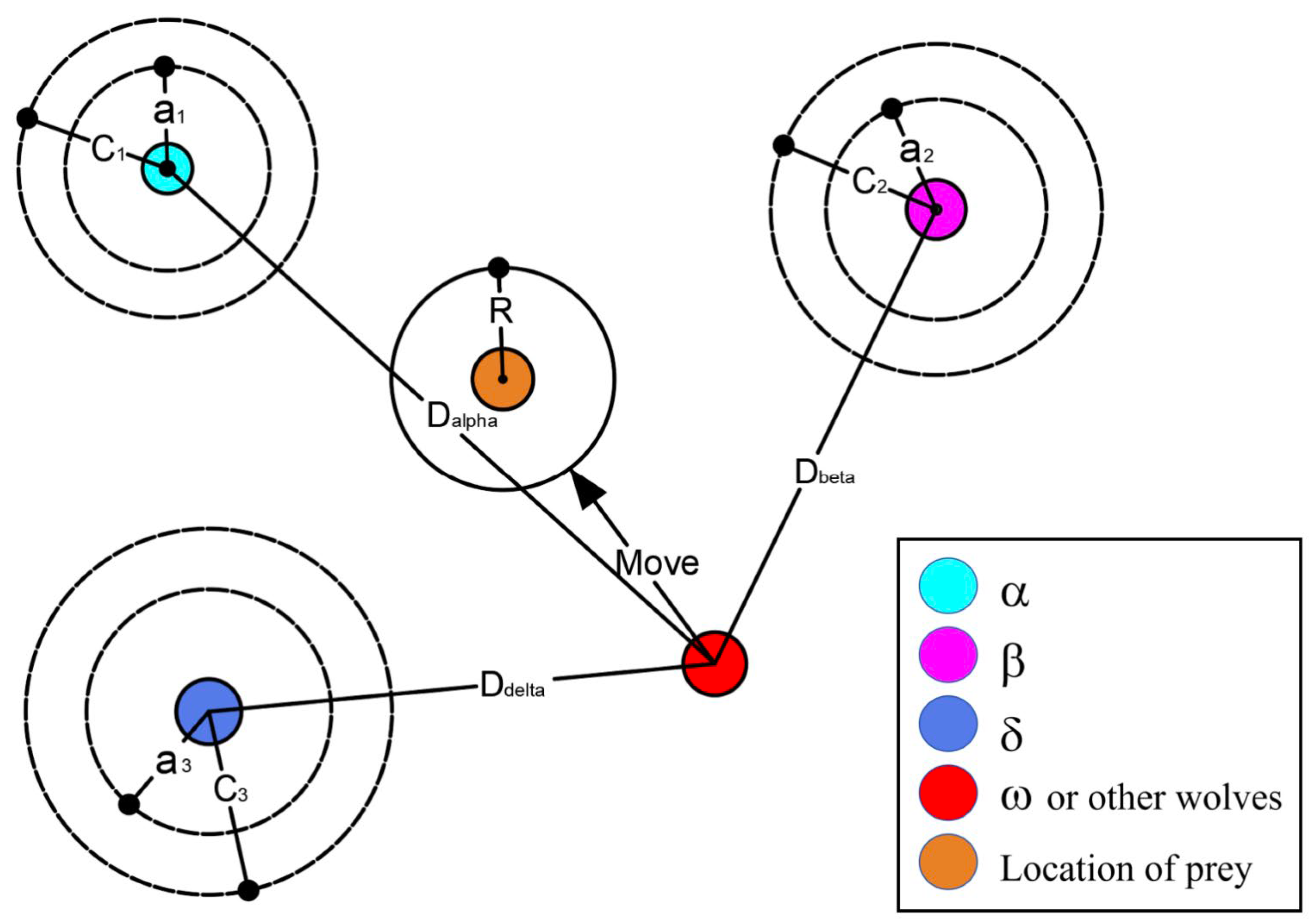
The method employed by members of a wolf pack to ascertain the prey’s position is depicted in Figure 2.
The mathematical formulation for how individual grey wolves ascertain the position of prey is delineated as follows: Equation (5) is employed to ascertain the distances between the pack members and the wolves α , β , and δ . Subsequently, Equation (8) synthesizes these calculations to identify the direction in which an individual grey wolf moves toward the prey.
D α = C 1 X α X ,   X 1 = X α A 1 D α D β = C 2 X β X ,   X 2 = X β A 2 D β D δ = C 3 X δ X ,     X 3 = X δ A 3 D δ
X t + 1 = X 1 + X 2 + X 3 3
where X α represents the position of α , X β denotes the position of β , X δ signifies the position of δ , C 1 , C 2 , a n d C 3 are random vectors, and X is the current position of the solution.

2.2. Improved Grey Wolf Optimizer (IGWO)

The Grey Wolf Optimizer (GWO) algorithm, notable for its simplicity, minimalistic parameter requirements, and robust convergence capabilities, has found initial applications across diverse fields including constraint optimization, drone route optimization, scheduling of module assembly, optimization of PI controllers, and workshop scheduling. However, the GWO algorithm faces challenges in maintaining a balance between its global and local search abilities. Furthermore, the optimal positioning of the leading wolf, a crucial element in directing the group, is not always guaranteed. These limitations often result in the algorithm prematurely converging to local optima and exhibiting slow convergence rates.
To overcome these challenges, the algorithm has undergone significant improvements:
  • Population Initialization Stage
The integration of cubic chaotic mapping with a refraction-based reverse learning strategy guarantees the diversity and uniqueness of the initial population. This approach effectively disperses initial solutions throughout the search space, mitigating the risk of early convergence on suboptimal solutions.
2.
Position Vector Update Stage
Adopting a nonlinear convergence factor instead of a linear one significantly improves the algorithm’s global and local search efficiency. This change enhances the wolves’ movement dynamics, enabling more effective exploration of the search space and the ability to escape local optima.
3.
Enhancements to Step Size and Leadership Influence
Adjusting the step size proportional weight and amplifying the role of the leading wolf allow the algorithm to circumvent local optima, thereby enhancing search efficacy and solution precision. Emphasizing the leading wolf’s position ensures the search is strategically oriented towards the most promising regions of the search space.
These strategic enhancements address the GWO algorithm’s inherent limitations, thereby bolstering its exploration and exploitation capabilities. This results in improved convergence speeds and higher accuracy in identifying optimal solutions, making the improved GWO algorithm a more effective tool for tackling complex optimization challenges.

2.2.1. The Integration of Cubic Chaotic Mapping and Reverse Learning Strategies

4.
Diversification of the Initial Population
The positioning of initial solutions plays a crucial role in determining an algorithm’s optimization efficacy and its ability to converge. Whereas traditional algorithms rely on pseudorandom number generators to position individuals across the solution space, this method often leads to an uneven distribution, causing overcrowding in certain regions. To mitigate this challenge, the introduction of chaos theory into the population initialization process marks a significant improvement. Its attributes of pseudorandomness, uniqueness, and thorough coverage ensure a more uniform distribution across the search space. The specific approach employs cubic chaotic mapping to delineate the initial population’s positions, enhancing the algorithm’s initial diversity and laying a robust foundation for the optimization journey. The formula utilized for this purpose is as follows:
2 y i + 1 = 4 y i 3 3 y i
1 < y i < 1 ,   y i 0 ,   i = 0,1 , , N
x i = X l b + X u b X l b y i + 1 2
where x i denotes the mapped position of a grey wolf individual, and X l b and X u b delineate the solution space’s lower and upper bounds, respectively. The process for initializing the grey wolf population through cubic chaotic mapping unfolds in several key steps: Firstly, commence by randomly generating a d-dimensional vector within the [−1,1] range, serving as the prototype individual. Then, apply Equation (7) to iterate over each dimension of the initial vector, thereby generating N − 1 subsequent individuals. Finally, utilize Equation (8) to transpose the values derived from cubic chaotic mapping into the coordinates of the grey wolf individuals.
5.
Elitization of the Initial Population
Enhancing the exploratory range of the initial population’s individuals and elevating the probability of identifying superior solutions necessitate the implementation of a lens imaging reverse learning technique. This method inverts the position of the current grey wolf individuals, yielding their lens imaging inverse solutions. If x j symbolizes the present grey wolf individual and x j denotes its lens imaging inverse solution, the relationship can be articulated as follows:
x j = a j + b j 2 + a j + b j 2 k x j k
where a j and b j are the minimum and maximum values found within the j dimension of the current population. The variable k represents the scaling factor of the lens, which is predetermined to be 12,000.
The initialization of the grey wolf population with the elite chaotic reverse learning strategy unfolds through a meticulously designed process:
  • Initial Population Creation
Begin by randomly generating N initial grey wolf individuals X = x i 1 , . . . , x i d , i = 1 , . . . , N , each denoting the i t h wolf’s position in the d t h dimension.
  • Chaotic and Reverse Transformations
Apply Equation (7) to perform a chaotic transformation on population X , resulting in a chaotic population Y . Concurrently, implement Equation (9) to execute a lens imaging reverse transformation on population X , yielding the lens imaging reverse population Z .
  • Elite Population Formation
Evaluate and rank the grey wolf individuals within populations Y and Z based on their fitness values. Select the top N individuals from this evaluation to assemble the elite chaotic reverse population P .
New Initial Population Selection: Sort the combined pool of individuals from population P and the original population X according to their fitness values. The foremost N individuals are then chosen to form the renewed initial grey wolf population.
X = x i 1 , , x i d

2.2.2. Nonlinear Convergence Factor

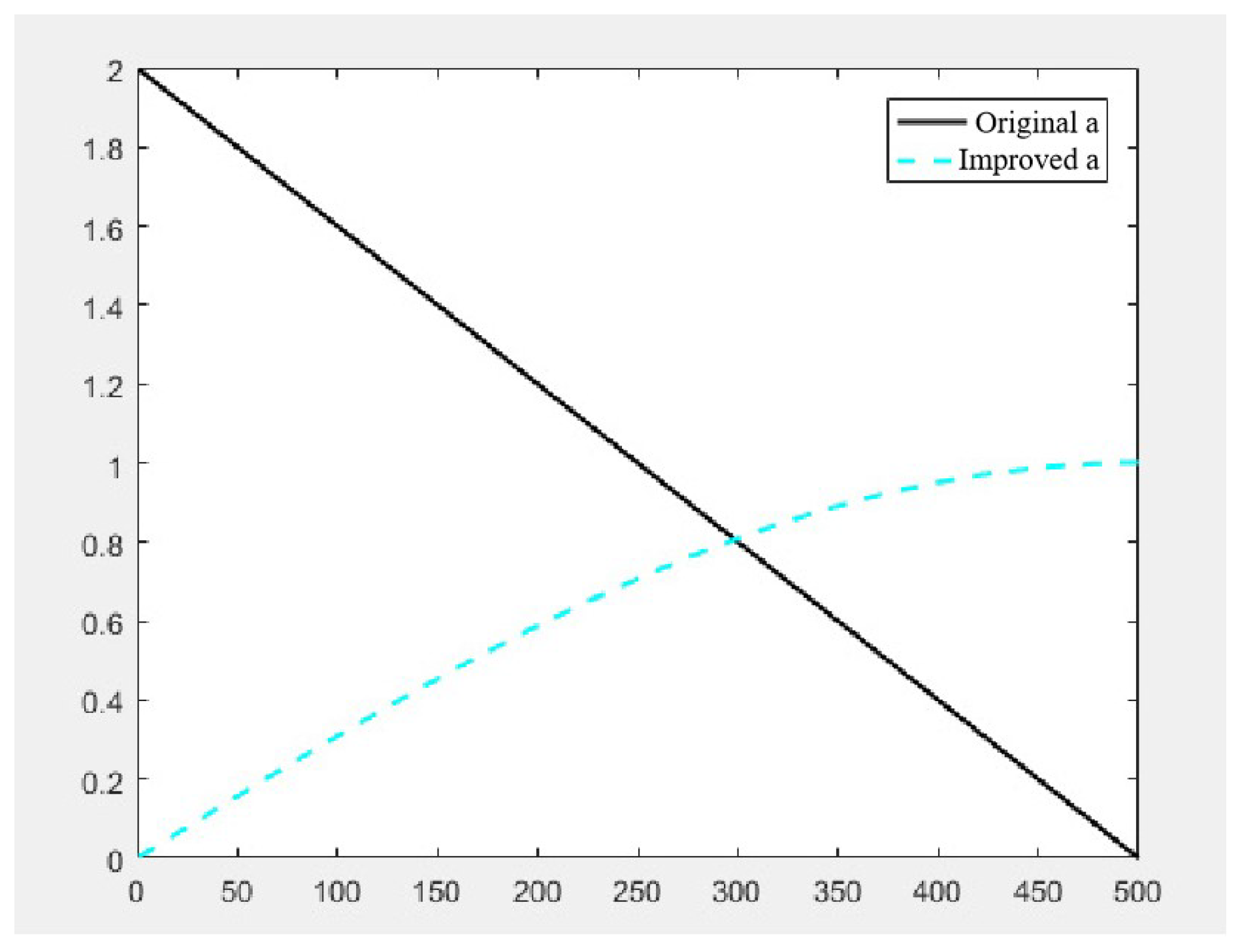
Introducing a nonlinear approach to modulating the convergence factor significantly boosts the algorithm’s proficiency in both global and local searches, thereby enhancing its efficiency in finding solutions. Traditionally, the Grey Wolf Optimizer (GWO) algorithm employs a linearly decreasing convergence factor a , which reduces with each iteration. This linear reduction might not adequately cater to the diverse demands of different search phases, occasionally resulting in premature convergence or entrapment in local optima [33]. By adopting a nonlinear function for adjusting a , the algorithm gains the flexibility to adapt its convergence rate in response to the evolving dynamics of the search process, as shown in Figure 3.
a = cos π 2 × 1 t t m a x
where t denotes the current iteration count within the optimization process, and t m a x specifies the upper limit on the total number of iterations allowed.

2.2.3. Adjusting the Position Update Mechanism

6.
Incorporating Step Size Proportional Weight
This introduces a novel approach utilizing a proportional weight derived from the Euclidean distance of the step size. The formulation is as follows:
W 1 = X 1 X 1 + X 2 + X 3 W 2 = X 2 X 1 + X 2 + X 3 W 3 = X 3 X 1 + X 2 + X 3
where W 1 , W 2 , and W 3 symbolize the learning rates by which the omega wolf ω adapts from the α , β , and δ wolves, respectively. To circumvent the risk of the algorithm becoming ensnared in local optima, an improvement has been made to the traditional GWO algorithm’s position update equation through the implementation of a dynamic weight strategy. This approach entails the derivation of proportional weights W 1 , W 2 , and W 3 from the position vectors, designed to undergo modifications in each iteration. Consequently, this strategy ensures that the pack’s leaders can dynamically steer the collective towards progressive movement.
7.
Enhancing the Significance of Position Updates by the Alpha Wolf
In population-based optimization algorithms, such as the Genetic Algorithm (GA) [34], Particle Swarm Optimization (PSO) [35], Artificial Bee Colony (ABC) [36], and Differential Evolution (DE) [37], achieving a balance between exploration and exploitation is essential. Exploration is the process of searching for new potential solutions within the search space, whereas exploitation optimizes search efficiency by leveraging existing, high-quality solutions. The Grey Wolf Optimizer (GWO) is typically constrained by a limitation wherein non-leader wolves, other than the α , β , and δ wolves, are predominantly attracted towards the trio of leader wolves. This dynamic often leads to premature convergence, resulting in the algorithm settling for local optima without sufficiently exploring the search space. To enhance the GWO’s efficacy, refining its position update mechanism is proposed to ensure a more effective balance between exploration and exploitation. This refinement utilizes the insights of the three leading wolves (alpha, explorer, and tracker) to direct candidate solutions towards the global optimum. By amplifying the alpha wolf’s role in position updating and the leading wolf’s overall influence, the algorithm’s capacity for optimization and precision in finding solutions is significantly improved.
X t + 1 = ρ 1 × ω 3 × W 1 × X 1 t + W 2 × X 2 t + W 3 × X 3 t 3 + ρ 2 × ω 4 × X b e s t X
where X b e s t denotes the α wolf’s position, and ω 3 and ω 4 refer to random numbers in the range of [0, 1]. ρ 1 and ρ 2 refer to random numbers in the range of (0, 1], which are employed to fine-tune the balance between exploration and exploitation capabilities.

3. Implementation

3.1. Evaluating the Enhanced Algorithm Through Tests and Simulations

3.1.1. Benchmark Functions

To evaluate the performance improvements of the Grey Wolf Optimizer, 10 standard international test functions from the literature [38] were selected for simulation tests of the IGWO. Detailed in Table 1, these functions are described by their names, formulas, dimensions, search domains, and optimal values. They represent a broad range of optimization problems, such as unimodal, multimodal, nonlinear, and non-convex scenarios, with f9 having a dimensionality of 30 and f10 a dimensionality of 2.

3.1.2. Evaluating IGWO Against Competing Algorithms

The Improved Grey Wolf Optimizer (IGWO) was assessed by calculating the mean and standard deviation of its performance on ten complex functions, both unimodal and multimodal. These metrics were then compared with those from the original Grey Wolf Optimizer (GWO), the Whale Optimization Algorithm (WOA) [39], and the Northern Goshawk Optimization (NGO) algorithms [40]. The comparative performance of these four algorithms is compiled in Table 2, where the superior outcomes are accentuated in bold.
Analyzing the data presented in Table 2 yields several insights:
8.
The IGWO algorithm outperforms the basic GWO, WOA, and NGO algorithms in terms of both accuracy and robustness, as evidenced by its mean values and standard deviations across all test functions.
9.
In dealing with unimodal functions ( f 1 f 5 ), the IGWO achieves global optimums or near-optimums more efficiently than its counterparts.
10.
When tackling multimodal functions ( f 6 f 10 ), the IGWO successfully navigates away from local optima to secure superior solutions, especially apparent in its performance on the Rastrigin ( f 7 ) and Griewank ( f 9 ) functions where it, alongside NGO, reaches the global optimum with minimal standard deviation. In contrast, the basic GWO is notably prone to settling at local optima.
11.
Overall, the IGWO algorithm’s results across various test functions attest to its excellent versatility and adaptability, showcasing its effectiveness in addressing optimization challenges of varying types and complexities.
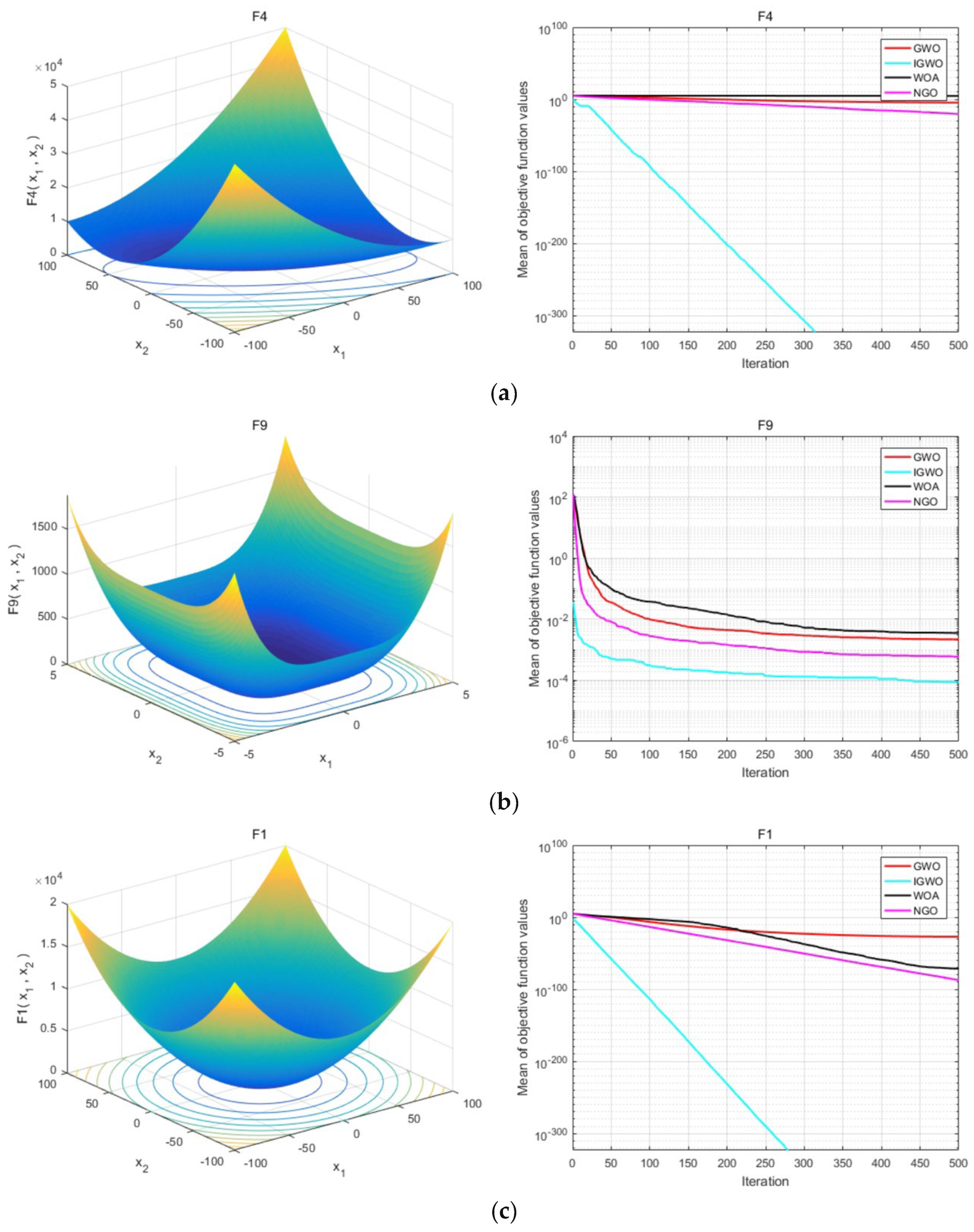
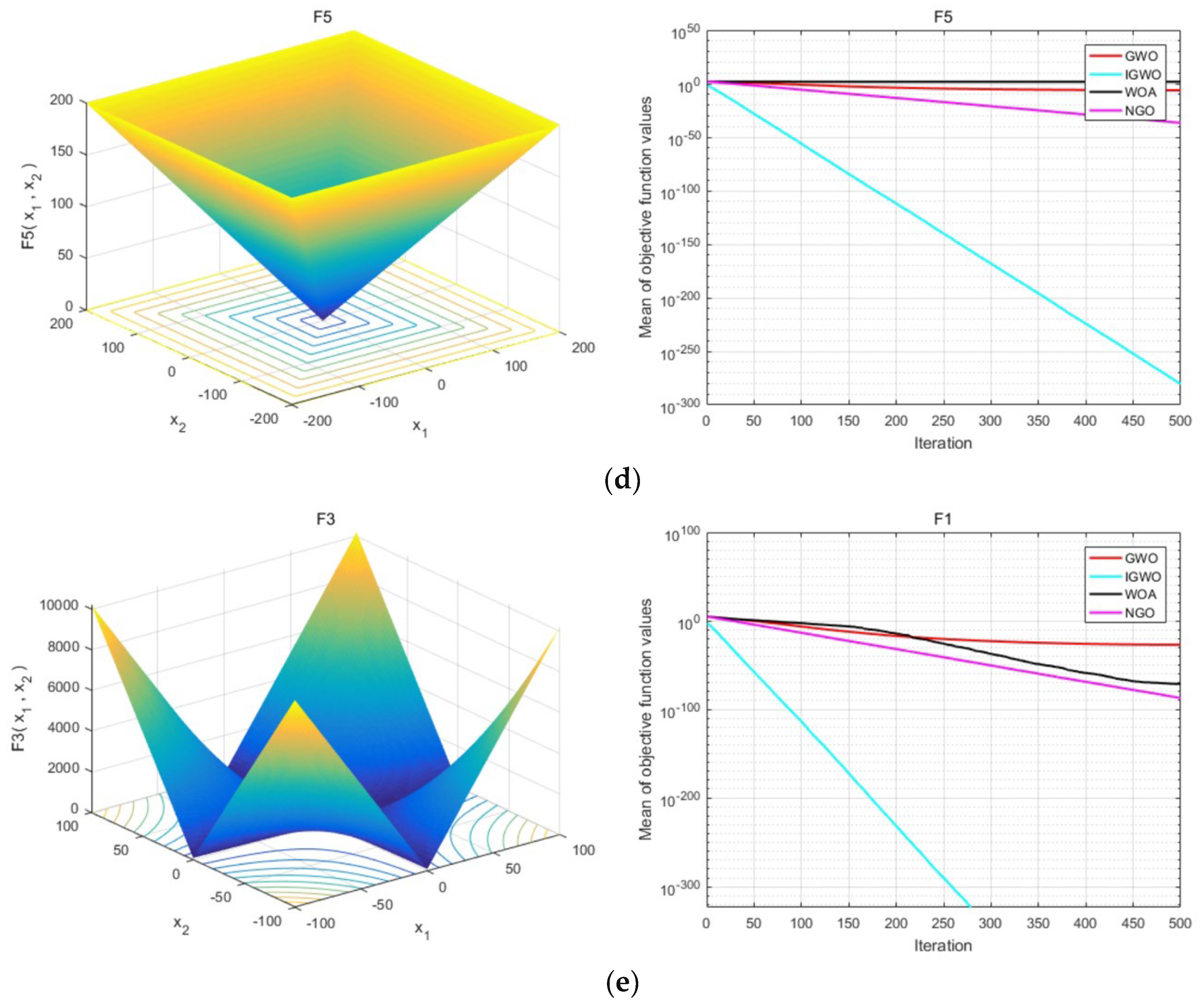
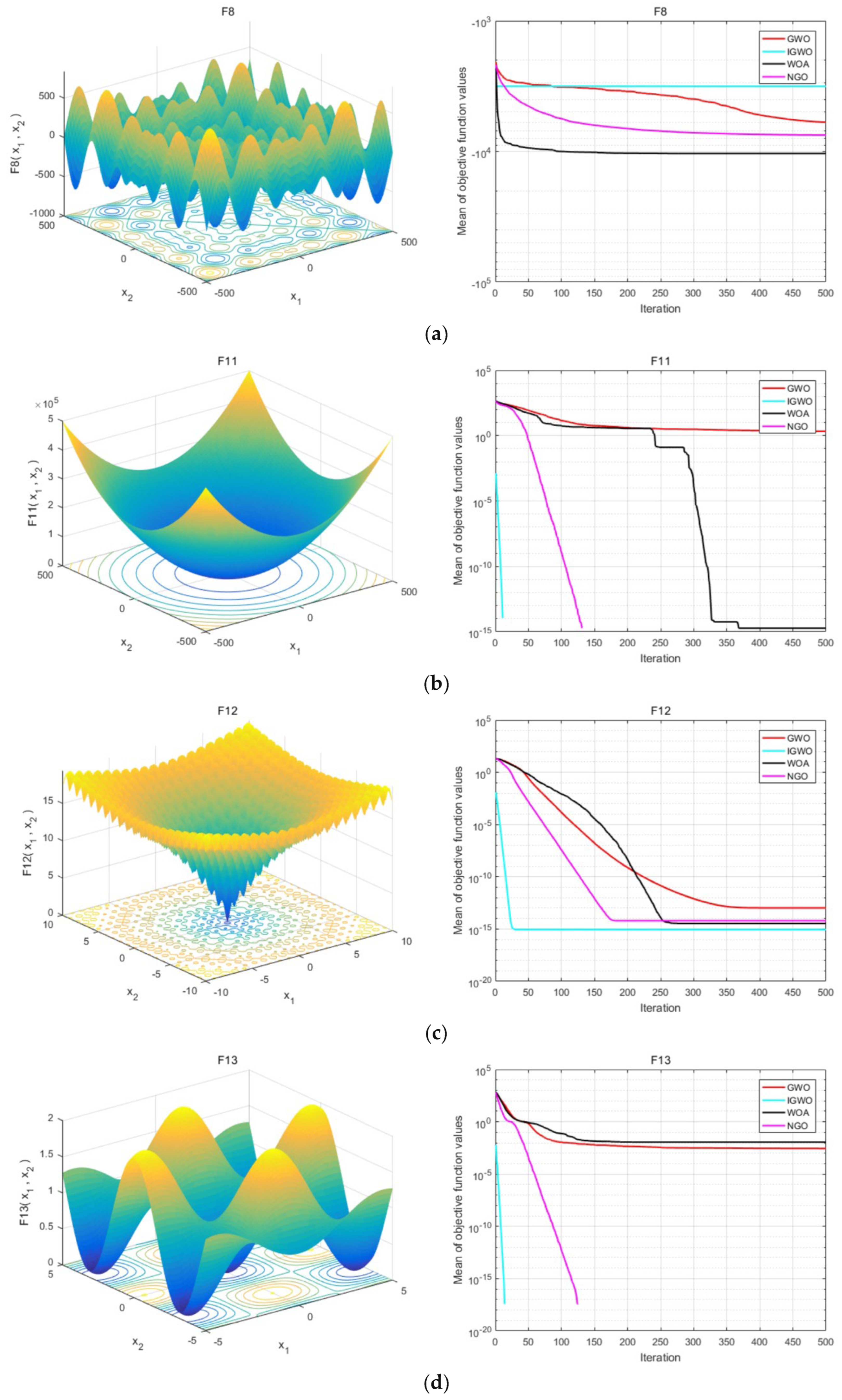
For a more detailed comparison of the IGWO algorithm’s optimization capabilities against those of the basic GWO, WOA, and NGO algorithms on unimodal test functions, fitness value change curves for these algorithms across functions f 1 f 5 are illustrated in Figure 4.
In all unimodal test functions, the IGWO algorithm consistently converges to the global optimum or very near it, with stable fitness value fluctuations. In contrast, the basic GWO, WOA, and NGO algorithms exhibit more significant variations and fluctuations in their fitness value trajectories on certain unimodal functions, indicating that these algorithms are more susceptible to becoming trapped in local optima or encountering difficulties in overcoming saddle points.
To further extend the comparative analysis to multimodal test functions, Figure 5 displays the trends in fitness values of the four algorithms on functions f 6 f 10 , illustrating their optimization performance in these scenarios.
The analysis presented in Figure 5 clearly shows that the IGWO algorithm outperforms the GWO, WOA, and NGO algorithms in optimizing multimodal functions, achieving exceptionally good results. This advantage is notably significant for functions f7, f8, and f10, where it managed a standard deviation of 0. Except in the f10 case, the IGWO algorithm has shown superior optimization capabilities.
These findings underscore the IGWO algorithm’s robust global search potential and its proficiency in overcoming local optima. It proves effective and exhibits high performance across a range of optimization challenges, regardless of their dimensionality or complexity, showcasing the efficacy of the enhancements made to the original algorithm.

4. Experiments and Analyses

4.1. Inverse Analysis of Tunnel Surrounding Rock Mechanical Parameters Based on IGWO-BP

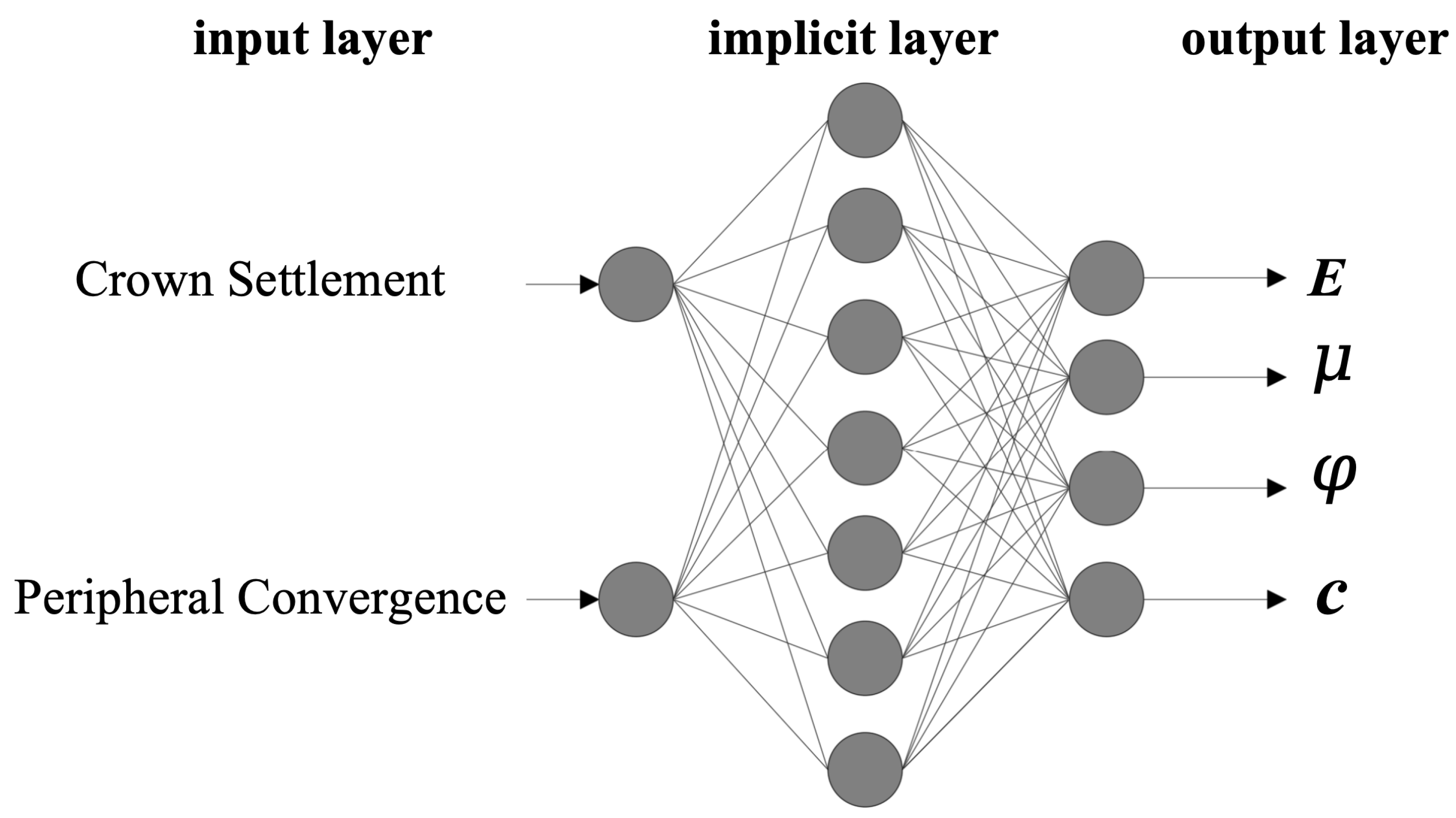
The neural network utilizes a tri-layer architecture for its computations, with the hidden layer’s neuron count m being ascertainable through the following empirical equation:
m = a + n + l
where a signifies the neuron count in the input layer, which is influenced by the number of displacement indicators and is thus 2. The variable n , indicating the neuron count in the output layer, depends on the number of inversion parameters, amounting to 4. Lastly, l stands as a constant valued between 1 and 10. The transition from the input to the hidden layer employs the logsig function—an S-shaped hyperbolic function—whereas the connection from the hidden layer to the output layer uses the purelin function—a linear function. Following this formula and through preliminary calculations, the hidden layer’s neuron count is finalized at 7.
The neural network structure model established for the inverse analysis of surrounding rock parameters of the Lotus Tunnel is illustrated in Figure 6 below.
The results from the 25 experimental configurations, identified via orthogonal testing, have been compiled. These results include both crown settlement and peripheral convergence displacement values, which serve as the input vectors for training. Concurrently, the mechanical parameters from each of these configurations are utilized as output vectors for training. This approach creates the IGWO-BP neural network’s training dataset, detailed in Table 3.
Utilizing the IGWO-BP neural network post-training, it is possible to inversely deduce the mechanical parameters of the surrounding rock [ E , μ , φ , c ] from rock deformation data, including crown settlement and peripheral convergence. This method completes the reverse analysis procedure. To assess the trained neural network’s reliability, real-world measurements from the YK37 + 330 section were used for verification. By inputting the measured values of crown settlement and peripheral convergence displacement from YK37 + 330 into the trained inversion model, the model provided predictions of the surrounding rock’s mechanical characteristics: an elastic modulus of 0.32 GPa, a Poisson’s ratio of 0.26, a cohesion of 156.14 kPa, and an internal friction angle of 28.52°.
This study adopts a simplified experimental scenario, focusing primarily on the behavior of elastic materials. The selection of this scenario aims to validate the basic effectiveness of the integration of the Improved Grey Wolf Optimization (IGWO) algorithm and the Backpropagation (BP) neural network in the inversion of surrounding rock mechanical parameters. Given the simplicity of the chosen scenario, the applicability of the results is currently limited to elastic material behavior, and further validation for non-elastic responses will require more complex experimental setups.

4.2. Forward Verification

4.2.1. Project Overview

The Lianhua Tunnel commences in the Xiangdong District of Pingxiang City and extends to Liushi Township in Lianhua County. Designed as a bifurcated tunnel, its left and right passages measure 3210 m and 3220 m in length, respectively. Surrounding rock classifications are divided into grades IV, V, and III. Specifically, grade IV rocks make up 47.6% of the tunnel’s entire length, grade V rocks account for 33.7%, and grade III rocks account for 18.7%. The deepest point of the tunnel lies at 317 m below the surface. Characterized by its shallow depth, wide span, and exceptional length, this structure is a notable example of a large-scale highway tunnel.

4.2.2. Developing the Tunnel Model

To address the issue of crown uplift deformation observed in the Lianhua Tunnel, the excavation interval from YK37 + 330 to YK37 + 370 was chosen for analysis. Utilizing information from geological exploration reports among other sources, a 3D numerical model in Midas GTS NX 2024 (New eXperience of Geo-Technical analysis System) for excavating this section of the tunnel was developed, illustrated in Figure 7. The model measures 100 m along the X-axis, 40 m along the Y-axis, and 70 m along the Z-axis, with each model boundary being at least five times the tunnel’s diameter away from the tunnel boundary itself, thereby satisfying numerical computation standards. The preliminary support structure is composed of steel arches, anchor bolts, and shotcrete, with anchor bolts represented by rod elements, shotcrete by plate elements, and steel arches by beam elements.
Model Layer Division: The geological construction and rock types mentioned in the project data led to a division of the model into two layers, the first being strongly weathered sandy shale and the second moderately weathered sandy shale.
Material Characteristics of the Model: For the rock and soil, the Mohr–Coulomb model dictates the material parameters, while anchor bolts and shotcrete are modeled using an elastic framework. Shotcrete is applied in the model to a thickness of 30 cm, and the benching method is chosen for excavation.
Boundary Conditions: The model’s bottom is constrained in all directions, ensuring stability; the sides are restricted horizontally, promoting lateral support; the top remains an unrestricted boundary, allowing for natural adjustment.
Mechanical Properties of Surrounding Rock and Tunnel Support Materials: Table 4 details the mechanical parameters used in this simulation for both the surrounding rock and the tunnel’s support materials. In an effort to accurately model the unloading of rock pressure post-excavation, a construction scenario was implemented where initial support is applied at intervals of 2 m, closely aligned with the benching excavation method. Load release coefficients of 0.4, 0.3, and 0.3 were established to mimic the gradual release of the surrounding rock’s load following excavation.
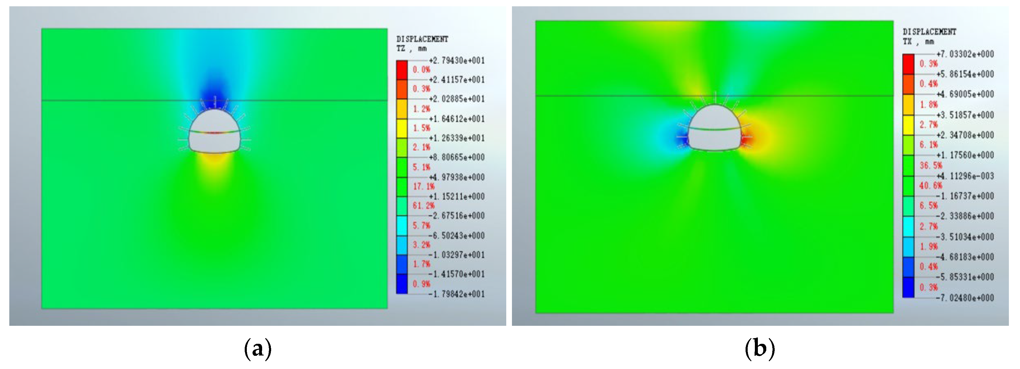
To evaluate the validity and credibility of the parameters obtained from inversion, forward verification was conducted. Using the mechanical parameter combinations derived from the inversion results at section YK37 + 330, a corresponding forward simulation model was developed with Midas GTS NX 2024 software. The mechanical parameters of surrounding rock, as determined by the inversion model, were inputted into the forward model. This approach enabled the calculation of vault settlement and peripheral convergence displacement values for section YK37 + 330. The results, depicted in a displacement cloud diagram, are presented in Figure 8.
The displacement from the numerical simulation’s forward verification was compared with the actual measured displacement. The comparison results are shown in Table 5.
The mechanical parameters of the surrounding rock were inverted using the displacement back-analysis method, and these parameters were subsequently applied in a forward model to calculate displacements for vault settlement and peripheral convergence. The forward model’s calculations yielded displacements of 17.98 mm for vault settlement and 7.02 mm for peripheral convergence. When compared with actual site monitoring data—17.12 mm for vault settlement and 6.74 mm for peripheral convergence—the relative errors were found to be 5.02% and 4.15%, respectively. This comparison demonstrates a close match between the forward model’s predictions and the real-world measurements, evidencing the model’s conservative accuracy. Thus, the mechanical parameters derived from the improved IGWO-BP model inversion are deemed to be highly accurate.
While it is hypothesized that the IGWO-BP method may offer potential advantages in handling more complex non-elastic responses, this assumption has yet to be validated through experimental data. Therefore, the conclusions of this study are based on the current elastic material testing scenario, and the applicability of the method to non-elastic responses will require further experimental investigation in future research.
In this study, the IGWO-BP (Improved Grey Wolf Optimizer with Backpropagation) method was chosen to handle elastic responses due to its advantages over traditional approaches. Although the rock mass response in the Lotus Tunnel is predominantly elastic, the IGWO-BP offers improved accuracy by overcoming the limitations of traditional methods, which rely on linear assumptions and are sensitive to initial conditions. By combining the global search capabilities of the Grey Wolf Optimizer with the nonlinear fitting abilities of the Backpropagation neural network, the IGWO-BP enhances parameter inversion accuracy, even in complex geotechnical scenarios.
This was evident when the parameters obtained from the IGWO-BP were applied in forward simulations to calculate roof settlement and surrounding convergence displacement. The simulation predicted a roof settlement of 17.98 mm, with a relative error of only 5.02% compared to the measured value of 17.12 mm. These results demonstrate the method’s effectiveness in handling elastic responses and providing reliable predictions in tunnel excavation.
Beyond elastic responses, the IGWO-BP also excels in modeling non-elastic behaviors, particularly in complex conditions. The Backpropagation neural network captures nonlinear material relationships, making the method well suited for handling non-elastic responses [41,42]. Additionally, the Grey Wolf Optimizer improves the method’s global search capability, ensuring more robust and accurate results, even when material responses deviate from linear behavior.

5. Conclusions

This study elaborates on the enhancement strategies for addressing the deficiencies of the Grey Wolf Algorithm, showcasing the successful integration of the refined algorithm with a BP neural network for the inverse analysis of surrounding rock parameters during tunnel excavation processes. The research unfolds across two pivotal sections:
12.
This research thoroughly analyzes the limitations of the Grey Wolf Algorithm and proposes an enhanced version, the Improved Grey Wolf Optimization (IGWO). This upgraded algorithm leverages cubic chaotic mapping and a refraction reverse learning strategy for optimizing the initial population, significantly improving data diversity and uniqueness. Moreover, by substituting the traditional linear convergence factor with a nonlinear one and introducing new parameters such as step size ratio weight and leading wolf weight, the algorithm notably enhances its ability to balance local and global search capabilities. This enhancement not only allows for a more effective escape from local optima but also substantially improves optimization efficiency and accuracy.
13.
In applying this to surrounding rock parameter inversion, the study utilizes an IGWO-optimized BP neural network model, incorporating orthogonal analysis methods to devise 25 numerical simulation experiments. These experiments, which take vault settlement and peripheral convergence data as inputs and output the mechanical parameters of surrounding rock, establish a reverse analysis model. The IGWO-BP neural network model’s effectiveness and accuracy in inverting surrounding rock parameters are confirmed by inverse analysis of actual data from YK37 + 330, achieving relative errors of 5.02% in vault settlement and 4.15% in peripheral convergence. These results highlight the model’s precision and practicality.
While this study demonstrates the successful integration of the Improved Grey Wolf Optimization (IGWO) algorithm with the Backpropagation (BP) neural network in the inversion of surrounding rock mechanical parameters, the experimental scenario is relatively simplified, primarily focusing on elastic material behavior. Consequently, the applicability of this method to non-elastic responses remains unverified. Future research will focus on extending the IGWO-BP method to more complex geological and mechanical conditions, with a particular emphasis on non-elastic scenarios, to evaluate its potential for broader applications in rock engineering.

Author Contributions

Q.C. led the academic direction. C.Z. developed the manuscript and wrote this paper. W.Z. conducted the investigation. X.H. reviewed this paper. All authors have read and agreed to the published version of the manuscript.

Funding

The authors gratefully acknowledge the financial support from The Science and Technology Program of Hunan Provincial Department of Transportation (no. 202308).

Institutional Review Board Statement

Not applicable.

Data Availability Statement

The datasets presented in this article are not readily available due to technical limitations. Requests to access the datasets should be directed to Chen Zhang.

Conflicts of Interest

The authors declare no conflicts of interest.

References

  1. Davarpanah, S.M.; Sharifzadeh, M.; Sattarvand, J.; Narimani, S. Evaluation of building displacement induced by EPB tunneling through GPS-GNSS monitoring system and back analysis technique (Tabriz Subway Twin Tunnels). Civ. Eng. J. 2016, 2, 270–285. [Google Scholar] [CrossRef]
  2. Deng, H.-S.; Fu, H.-L.; Shi, Y.; Zhao, Y.-Y.; Hou, W.-Z. Countermeasures against large deformation of deep-buried soft rock tunnels in areas with high geostress: A case study. Tunn. Undergr. Space Technol. 2022, 119, 104238. [Google Scholar] [CrossRef]
  3. Ferrero, A.M.; Migliazza, M.; Segalini, A.; Gullì, D. In situ stress measurements interpretations in large underground marble quarry by 3D modeling. Int. J. Rock Mech. Min. Sci. 2013, 60, 103–113. [Google Scholar] [CrossRef]
  4. Kirsten, H. Determination of rock mass elastic moduli by back analysis of deformation measurements. Explor. Rock Eng. 1976, 1, 165–172. [Google Scholar]
  5. Sakurai, S.; Abe, S. A design approach to dimensioning underground openings. In Proceedings of the 3nd International Conference on Numerical Methods in Geomechanics, Aachen, Germany, 2–6 April 1979. [Google Scholar]
  6. Gioda, G.; Maier, G. Direct search solution of an inverse problem in elastoplasticity: Identification of cohesion, friction angle and in situ stress by pressure tunnel tests. Int. J. Numer. Methods Eng. 1980, 15, 1823–1848. [Google Scholar] [CrossRef]
  7. Sakurai, S.; Takeuchi, K. Back analysis of measured displacements of tunnels. Rock Mech. Rock Eng. 1983, 16, 173–180. [Google Scholar] [CrossRef]
  8. Yang, Z.; Liu, Z. The elementary applications of back-analysis from displacements in designs of underground engineering. Undergr. Eng. 1981, 2, 20–24. [Google Scholar] [CrossRef]
  9. Guo, H.Z.; Ma, Q.C.; Xue, X.C.; Wang, D. The analytical method of the initial stress field for rock masses. Chin. J. Geotech. Eng. 1983, 5, 64–75. (In Chinese) [Google Scholar]
  10. Feng, X.; Zhang, Z.; Yang, C.X.; Lin, Y.M. Study on genetic neural network method of displacement back analysis. Chin. J. Rock Mech. Eng. 1999, 18, 529–633. [Google Scholar]
  11. Ravandi, E.G.; Rahmannejad, R.; Monfared, A.E.; Ravandi, E.G. Application of numerical modeling and genetic programming to estimate rock mass modulus of deformation. Int. J. Min. Sci. Technol. 2013, 23, 733–737. [Google Scholar] [CrossRef]
  12. Miro, S.; König, M.; Hartmann, D.; Schanz, T. A probabilistic analysis of subsoil parameters uncertainty impacts on tunnel-induced ground movements with a back-analysis study. Comput. Geotech. 2015, 68, 38–53. [Google Scholar] [CrossRef]
  13. Gao, W.; Chen, D.; Dai, S.; Wang, X. Back analysis for mechanical parameters of surrounding rock for underground roadways based on new neural network. Eng. Comput. 2018, 34, 25–36. [Google Scholar] [CrossRef]
  14. Wan, Z.; Huang, Y.; Zhu, Z.; Wang, T.; Jing, J.; Xiao, L. Back analysis on mechanical parameters of RCC dam during operation period in alpine region. Water Conserv. Hydropower Technol. 2017, 48, 50–55. [Google Scholar]
  15. Zhuang, D.; Ma, K.; Tang, C.; Liang, Z.; Wang, K.; Wang, Z. Mechanical parameter inversion in tunnel engineering using support vector regression optimized by multi-strategy artificial fish swarm algorithm. Tunn. Undergr. Space Technol. 2019, 83, 425–436. [Google Scholar] [CrossRef]
  16. Liu, J.; Weng, X.J.; Zhang, L.S.; Zhang, L.Z. Inversion of mechanical parameters of tunnel surrounding rock based on GA-BP neural network. Chin. J. J. Highw. Transp. Res. Dev. 2020, 37, 90–96. [Google Scholar]
  17. Cui, J.; Wu, S.; Cheng, H.; Kui, G.; Zhang, H.; Hu, M.; He, P. Composite interpretability optimization ensemble learning inversion surrounding rock mechanical parameters and support optimization in soft rock tunnels. Comput. Geotech. 2024, 165, 105877. [Google Scholar] [CrossRef]
  18. Zhao, H.; Feng, X. Study on genetic-support vector machine in displacement back analysis. Chin. J. Rock Mech. Eng. 2003, 22, 1618–1622. [Google Scholar]
  19. Zhou, G.; Sun, Y.; Jia, P. Application of genetic algorithm based BP neural network to parameter inversion of surrounding rock and deformation prediction. Mod. Tunn. Technol. 2018, 55, 107–113. [Google Scholar]
  20. Gao, W. Back analysis algorithm in geotechnical engineering based on particle swarm optimization. Yantu Lixue Rock Soil Mech. 2006, 27, 795–798. [Google Scholar]
  21. Kai, W.; Qian, S.; Song, M.E. A model of PSO-LSSVM and its application to displacement back analysis. Rock Soil Mech. 2009, 30, 1109–1114. [Google Scholar]
  22. Qi, Z.; Jiang, Q.H.; Zhou, C.B.; Xiang, B.Y.; Shao, J.D. A new slope displacement back analysis method based on v-SVR and MVPSO algorithm and its application. Chin. J. Rock Mech. Eng. 2013, 32, 1185–1196. [Google Scholar]
  23. Mirjalili, S.; Mirjalili, S.M.; Lewis, A. Grey wolf optimizer. Adv. Eng. Softw. 2014, 69, 46–61. [Google Scholar] [CrossRef]
  24. Saremi, S.; Mirjalili, S.Z.; Mirjalili, S.M. Evolutionary population dynamics and grey wolf optimizer. Neural Comput. Appl. 2015, 26, 1257–1263. [Google Scholar] [CrossRef]
  25. Gholizadeh, S. Optimal design of double layer grids considering nonlinear behaviour by sequential grey wolf algorithm. J. Optim. Civ. Eng. 2015, 5, 511–523. [Google Scholar]
  26. Jayabarathi, T.; Raghunathan, T.; Adarsh, B.; Suganthan, P.N. Economic dispatch using hybrid grey wolf optimizer. Energy 2016, 111, 630–641. [Google Scholar] [CrossRef]
  27. Heidari, A.A.; Pahlavani, P. An efficient modified grey wolf optimizer with Lévy flight for optimization tasks. Appl. Soft Comput. 2017, 60, 115–134. [Google Scholar] [CrossRef]
  28. Kumar, V.; Kumar, D. An astrophysics-inspired grey wolf algorithm for numerical optimization and its application to engineering design problems. Adv. Eng. Softw. 2017, 112, 231–254. [Google Scholar] [CrossRef]
  29. Wang, X.; Zhao, H.; Han, T.; Zhou, H.; Li, C. A grey wolf optimizer using Gaussian estimation of distribution and its application in the multi-UAV multi-target urban tracking problem. Appl. Soft Comput. 2019, 78, 240–260. [Google Scholar] [CrossRef]
  30. Kamboj, V.K. A novel hybrid PSO–GWO approach for unit commitment problem. Neural Comput. Appl. 2016, 27, 1643–1655. [Google Scholar] [CrossRef]
  31. Turabieh, H. A hybrid ANN-GWO algorithm for prediction of heart disease. Am. J. Oper. Res. 2016, 6, 136–146. [Google Scholar] [CrossRef]
  32. Zhang, X.; Kang, Q.; Cheng, J.; Wang, X. A novel hybrid algorithm based on biogeography-based optimization and grey wolf optimizer. Appl. Soft Comput. 2018, 67, 197–214. [Google Scholar] [CrossRef]
  33. Padhy, S.; Panda, S.; Mahapatra, S. A modified GWO technique based cascade PI-PD controller for AGC of power systems in presence of plug in electric vehicles. Eng. Sci. Technol. Int. J. 2017, 20, 427–442. [Google Scholar] [CrossRef]
  34. Moscato, P. On evolution, search, optimization, genetic algorithms and martial arts: Towards memetic algorithms. Caltech Concurr. Comput. Program C3P Rep. 1989, 826, 37. [Google Scholar]
  35. Wang, D.; Tan, D.; Liu, L. Particle swarm optimization algorithm: An overview. Soft Comput. 2018, 22, 387–408. [Google Scholar] [CrossRef]
  36. Karaboga, D.; Basturk, B. A powerful and efficient algorithm for numerical function optimization: Artificial bee colony (ABC) algorithm. J. Glob. Optim. 2007, 39, 459–471. [Google Scholar] [CrossRef]
  37. Price, K.V. Differential evolution. In Handbook of Optimization: From Classical to Modern Approach; Springer: Berlin/Heidelberg, Germany, 2013; pp. 187–214. [Google Scholar]
  38. Song, H.M.; Sulaiman, M.H.; Mohamed, M.R. An application of grey wolf optimizer for solving combined economic emission dispatch problems. Int. Rev. Model. Simul. 2014, 7, 838–844. [Google Scholar]
  39. Mirjalili, S.; Lewis, A. The whale optimization algorithm. Adv. Eng. Softw. 2016, 95, 51–67. [Google Scholar] [CrossRef]
  40. Dehghani, M.; Hubálovský, Š.; Trojovský, P. Northern goshawk optimization: A new swarm-based algorithm for solving optimization problems. IEEE Access 2021, 9, 162059–162080. [Google Scholar] [CrossRef]
  41. Zhang, X.; Yu, L.; Wang, M.; Yang, H. Mechanical response and failure characteristics of tunnels subjected to reverse faulting with nonuniform displacement: Theoretical and numerical investigation. Eng. Fail. Anal. 2024, 156, 107809. [Google Scholar] [CrossRef]
  42. Song, Z.; Yang, Z.; Huo, R.; Zhang, Y. Inversion analysis method for tunnel and underground space engineering: A short review. Appl. Sci. 2023, 13, 5454. [Google Scholar] [CrossRef]
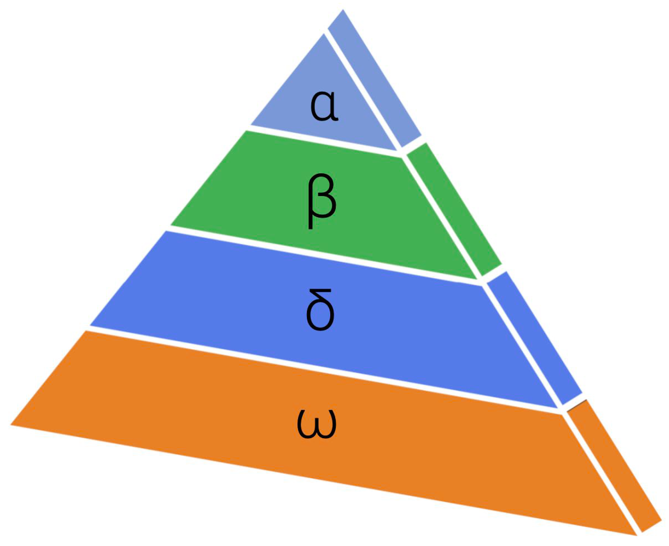
Figure 1. The hierarchy of the grey wolf.
Applsci 15 00537 g001
Figure 2. Grey wolf update location.
Applsci 15 00537 g002
Figure 3. Comparison chart of convergence factor.
Applsci 15 00537 g003
Figure 4. Comparison of function plot and convergence curve of single–peaked function. (a) f1–Schwefel 1.2 Function; (b) f2–Quartic Function; (c) f3–Sphere Function; (d) f4–Schwefel 2.21 Function; (e) f5–Schwefel 2.22 Function.
Applsci 15 00537 g004aApplsci 15 00537 g004b
Figure 5. Comparison of function plot and convergence curve of multi–peak function. (a) f6–Schwefel 2.26 Function; (b) f7–Rastrigin Function; (c) f8–Ackley Function; (d) f9–Griewank Function; (e) f10–Goldstein Price Function.
Applsci 15 00537 g005aApplsci 15 00537 g005b
Figure 6. Neural network model of inversion of surrounding rock.
Applsci 15 00537 g006
Figure 7. Three-dimensional model diagram.
Applsci 15 00537 g007
Figure 8. YK37 + 330 cross section forward inspection model displacement cloud map. (a) Crown settlement; (b) Peripheral convergence.
Applsci 15 00537 g008
Table 1. Set of common test functions.
Function NameFunction ExpressionSearch Rangefmin
Schwefel 1.2 f 1 ( x ) = i = 1 n   ( j = 1 i   x j ) 2 [−100, 100]0
Quartic f 2 ( x ) = i = 1 n   i x i 4 + r a n d o m [ 0,1 ) [−1.28, 1.28]0
Sphere f 3 ( x ) = i = 1 n   x i 2 [−100, 100]0
Schwefel 2.21 f 4 ( x ) =   m a x i { x i , 1 i n } [−100, 100]0
Schwefel 2.22 f 5 ( x ) = i = 1 n x i + i = 1 n x i [−10, 10]0
Schwefel 2.26 f 6 = i = 1 n   x i sin ( x i ) [−500, 500]−12,569.5
Rastrigin f 7 ( x ) = i = 1 n   [ x i 2 10 cos ( 2 π x i ) + 10 ] [−5.12, 5.12]0
Ackley f 8 ( x ) = 20 exp ( 0.2 1 n i = 1 n   x i 2 ) exp ( 1 n i = 1 n   cos ( 2 π x i ) ) + 20 + e [−32, 32]0
Griewank f 9 = 1 4000 i = 1 n   x i 2 i = 1 n   cos ( x i i ) + 1 [−50, 50]0
Goldstein Price f I 0 = [ 1 + ( x 1 + x 2 + 1 ) 2 m ] × [ 30 + ( 2 x 1 3 x 2 ) 2 n ] m = ( 19 14 x 1 + 3 x 1 2 14 x 2 + 6 x 1 x 2 + 3 x 2 2 ) n = ( 18 32 x 1 + 12 x 1 2 + 48 x 2 36 x 1 x 2 + 27 x 2 2 ) [−2, 2]3
Table 2. Experimental results of different GWO algorithms for 10 test functions.
Function GWOWOANGOIGWO
f1Mean3.9762 × 10−647,898.13851.1477 × 10−220
Standard Deviation9.4465 × 10−610,779.68384.0563 × 10−220
f2Mean0.00199890.00359840.000706327.1205 × 10−5
Standard Deviation0.00124690.00544880.000308366.8094 × 10−5
f3Mean1.0125 × 10−272.3525 × 10−727.7076 × 10−880
Standard Deviation1.5709 × 10−271.2881 × 10−711.2394 × 10−870
f4Mean6.7115 × 10−738.16111.2477 × 10−373.1068 × 10−279
Standard Deviation4.8223 × 10−729.0441.023 × 10−370
f5Mean1.06 × 10−166.8394 × 10−521.2728 × 10−457.4703 × 10−305
Standard Deviation8.6006 × 10−172.2572 × 10−511.3106 × 10−450
f6Mean−5818.9213−10,324.6818−7637.5386−3466.9346
Standard Deviation795.44921763.6363613.4378118.4035
f7Mean1.176000
Standard Deviation2.3394000
f8Mean1.019 × 10−134.6777 × 10−156.6909 × 10−158.8818 × 10⁻¹⁶
Standard Deviation1.694 × 10−142.9405 × 10−151.7413 × 10−150
f9Mean0.00223840.01072300
Standard Deviation0.0060780.04084700
f10Mean5.733599.8247
Standard Deviation14.78858.3808 × 10−51.2802 × 10−150.019301
Table 3. IGW0-BP training sample set.
Test NumberOutput VectorInput Vector
c / kPa φ / ( ° ) E / GPa μ Crown SettlementPeripheral Convergence
180202000.3217.828.44
280222500.3414.286.74
380243000.3611.785.58
480263500.389.984.74
580284000.4012.236.84
6110202500.3610.145.62
7110223000.388.614.63
8110243500.407.464.08
9110264000.3210.186.78
10110282000.348.425.07
11140203000.407.194.33
12140223500.326.293.76
13140244000.348.386.30
14140262000.367.255.16
15140282500.386.374.06
16170203500.345.683.54
17170224000.367.585.99
18170242000.386.664.97
19170262500.405.984.26
20170283000.325.303.42
21200204000.387.115.81
22200222000.406.324.82
23200242500.325.724.18
24200263000.345.243.66
25200283500.3217.828.44
Table 4. Table of mechanical parameters of surrounding rock and support.
Material E / GPa μ c / kPa φ / ( ° ) Unit Weight/kN/m3
First Soil Layer0.40.35502020
Second Soil Layer—— *20
Anchor Bolts/
Steel Arches
2100.3--78.5
Shotcrete280.2--24
*: To be inverted.
Table 5. Comparison results between forward model displacement and measured displacement.
Pile NumberMonitoring ItemsMeasured Values/mmCalculated Values/mmError/%Inversion Parameters
E / GPa μ c / kPa φ / ( ° )
YK37 + 330Crown Settlement17.1217.985.020.320.26156.1428.52
Peripheral Convergence6.747.024.15
Disclaimer/Publisher’s Note: The statements, opinions and data contained in all publications are solely those of the individual author(s) and contributor(s) and not of MDPI and/or the editor(s). MDPI and/or the editor(s) disclaim responsibility for any injury to people or property resulting from any ideas, methods, instructions or products referred to in the content.