Inertial Forces and Friction in Propulsion of a Rigid Body

Abstract

Inertially driven or vibration-driven capsule robots have recently attracted attention from various areas of science and engineering. The main advantage of such a mobile system is the lack of any external driving mechanism, which allows for an encapsulated construction and efficient operation in demanding environments. This study focuses on the conception of a mechanical system whose motion on a rough horizontal plane is caused only by the rotation of two internal masses. The mathematical model of the robot is presented in the non-dimensional form. The conditions for motion are formulated, and the working region of the system is specified. The active phase of the robot dynamics may include both forward motion and minor backward motion, or forward motion exclusively. Extensive numerical studies are conducted using two friction models. The numerical solutions to the dynamic problem are analyzed with regard to the total displacement and the average velocity per period of excitation. The interplay between model parameters is studied. The resulting maps on the parameter planes allow for substantial improvement in the robot performance. Moreover, it is demonstrated that the Stribeck effect occurring in the friction characteristics plays a positive role in the efficient motion of the system.

1. Introduction

The propulsion mechanism of mobile robots, designed as closed capsules without external moving parts or openings, has attracted considerable attention in recent research. Such robots can be conceptualized as enclosed structures containing one or more internal masses capable of oscillatory motion. By controlling the dynamics of these internal movements—either linear or rotational—the entire system can achieve directed motion. The underlying principle involves the generation of controlled inertial forces, which modulate both the normal force exerted by the robot on the surface and the resulting propulsion force. Commonly referred to as vibration-driven or inertia-driven robots, these systems offer significant advantages over traditional locomotion methods by eliminating the need for wheels, legs, or tracks. Their sealed design enhances robustness and facilitates operation in challenging environments, including solid and fluid media.

The theoretical foundations of such systems were extensively studied by Chernous’ko, who analyzed the dynamics and optimal control of rigid bodies equipped with internal moving masses. In paper [1], a simplified mechanical model was proposed, consisting of a rigid body capable of horizontal motion with an internally oscillating mass. Parameters for maximizing the system’s average velocity were derived. Subsequent work [2] investigated controlled horizontal motion under dry friction forces, where the movement of a bounded internal mass provided propulsion. In paper [3], the periodic translational motion of a two-mass system—comprising a container interacting with its environment and an internal moving mass—was examined. The study demonstrated how simple oscillatory motions of the internal mass induced displacement of the entire system. Experimental validation of this principle was achieved using pendulum systems and rotating masses in mobile robots designed for tubular environments.

Further advancements were made by Bolotnik et al. [4,5,6], who analyzed the dynamics of systems with two internal movable masses. Their work addressed optimal control problems for motion on rough surfaces, where horizontal and vertical movements of internal masses were used to regulate frictional forces and optimize velocity. These studies considered various friction laws, including piecewise linear, quadratic, and Coulomb friction. The results demonstrate that by modulating the internal masses’ dynamics, the external reaction forces could be controlled, enabling directed motion and velocity regulation.

The simplicity and versatility of vibration-driven robots make them promising candidates for a range of applications, including locomotion on surfaces, in dense media (e.g., soil), and within pipes. Potential biomedical applications include microrobots for drug delivery or diagnostic purposes. For instance, Bolotnik et al. [7] presented optimal control strategies for two-body systems in nonlinear viscous media, while Fang and Xu [8,9] explored similar setups in resistive environments, including interconnected modular systems.

Optimization challenges for these systems have been addressed in various contexts. Figurina [10] studied linear motion on inclined surfaces, while Sobolev and Sorokin [11] conducted experimental research on systems with unbalanced rotors. Sakharov [12] examined systems comprising rigid bodies and internal movable masses on rough surfaces, emphasizing rotational dynamics and friction modelling. Bardin and Panev [13,14] provided a comprehensive analysis of periodic motion induced by rotating unbalanced masses, identifying stable motion modes. Semendyaev and Tsyganov [15] investigated systems with eccentrics (unbalanced rotating wheels), achieving incremental motion on rough surfaces.

The idea of an inertial propulsion system can be used in various mixed mobile solutions. For example, recently, Timofte et al. [16] have investigated an inertial drive of a wheeled platform based on two revolving eccentric bodies. More generally, a critical review of various human efforts to generate thrust using rotating masses has been provided by Provatidis [17].

This study demonstrates that oscillatory internal movements of small masses enable locomotion on horizontal surfaces through the interaction of dry friction forces. The proposed approach is also applicable to motion within resistive media governed by different resistance laws. The primary objective of this research is to determine the effect of different factors on dynamics of such systems, which is crucial in developing effective strategies for initiating and controlling their motion. To the best knowledge of the authors, such an extensive parameter analysis corresponding to the proposed inertial drive has not been presented yet by other researchers.

This paper is divided into five sections. The conceptual and mathematical model of the considered system are presented in Section 2. The basic analytical studies focused on the conditions for motion of the system are discussed in Section 3. Next, in Section 4, the results of series of numerical experiments with different models of dry friction are reported. Finally, concluding remarks are formulated in Section 5.

2. Problem Formulation and Mathematical Model

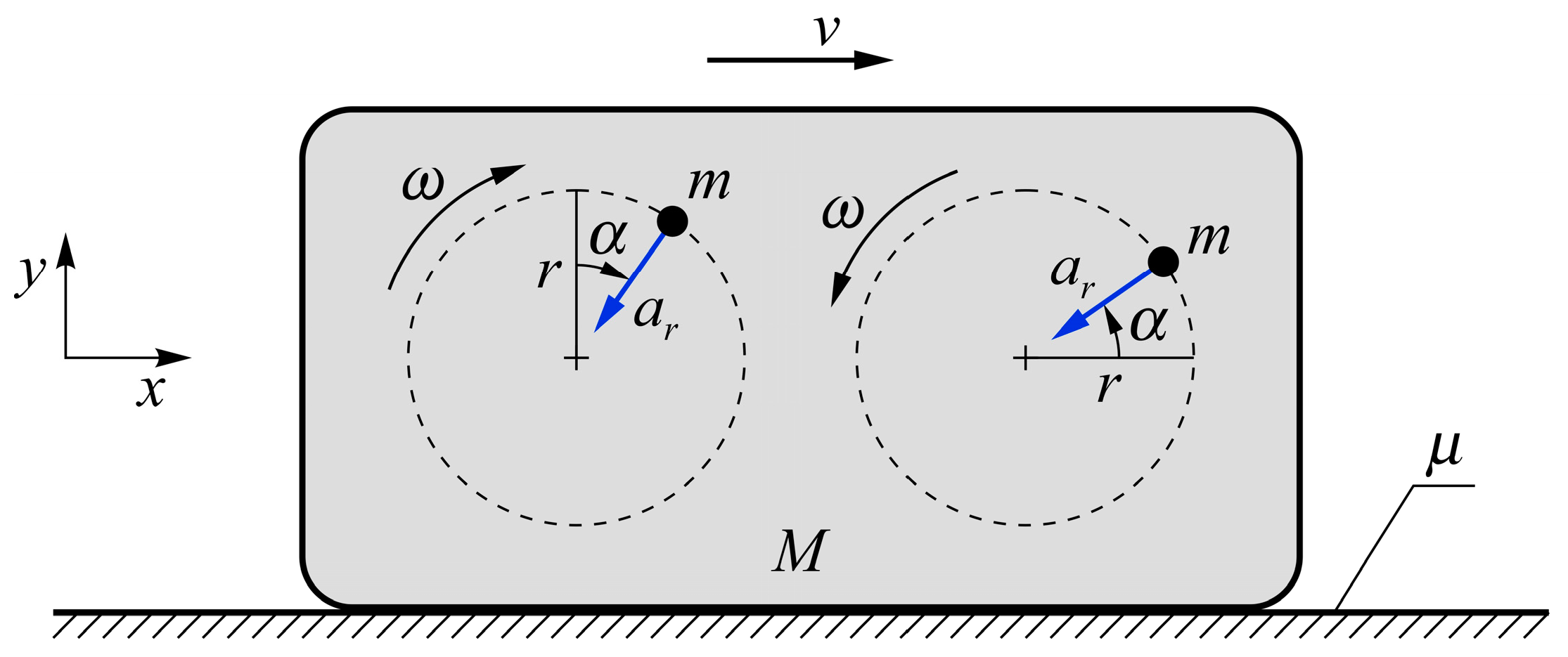
The concept of a body moving due to the inertial drive is schematically illustrated in Figure 1. The mechanical system consists of a rigid main body (a box or a capsule) of mass M and two internal masses treated as material points (particles), each having mass m. The box is placed on a rough horizontal plane and can move along the x axis. Its interaction with the flat ground is described with the dry friction coefficient μ. The internal masses, in turn, revolve in circles of radius r about the axes fixed to the box. Both particles move in opposite directions with a constant common angular speed ω, which is controlled by appropriate driving torques. Positions of the point masses are specified by the angle α.

The particles in circular motion undergo the normal (radial) accelerations relative to the box, a_r = rω². As a reaction, forces F₁ and F₂ of an inertial nature are exerted on the box. They play the crucial role in causing the robot to move. Continuously alternating directions of F₁ and F₂ lead to cyclic changes in the overall load on the ground (and the friction force), as well as to cyclic generation of the propelling force. The basic problem is to choose such values of the model parameters that ensure efficient and smooth motion of the whole system.

Consider the circular motion of the particles. The Cartesian components of the inertial forces are given by

$$F_{1x}=F_{2y}=mr{\omega }^2\sin \left(\alpha \right), F_{1y}=F_{2x}=mr{\omega }^2\cos \left(\alpha \right).$$

(1)

Consequently, the total inertial force F acting on the box has the following equal components:

$$F_x=F_y=mr{\omega }^2\left[\sin \left(\alpha \right)+\mathrm{c}\mathrm{o}\mathrm{s}\left(\alpha \right)\right].$$

(2)

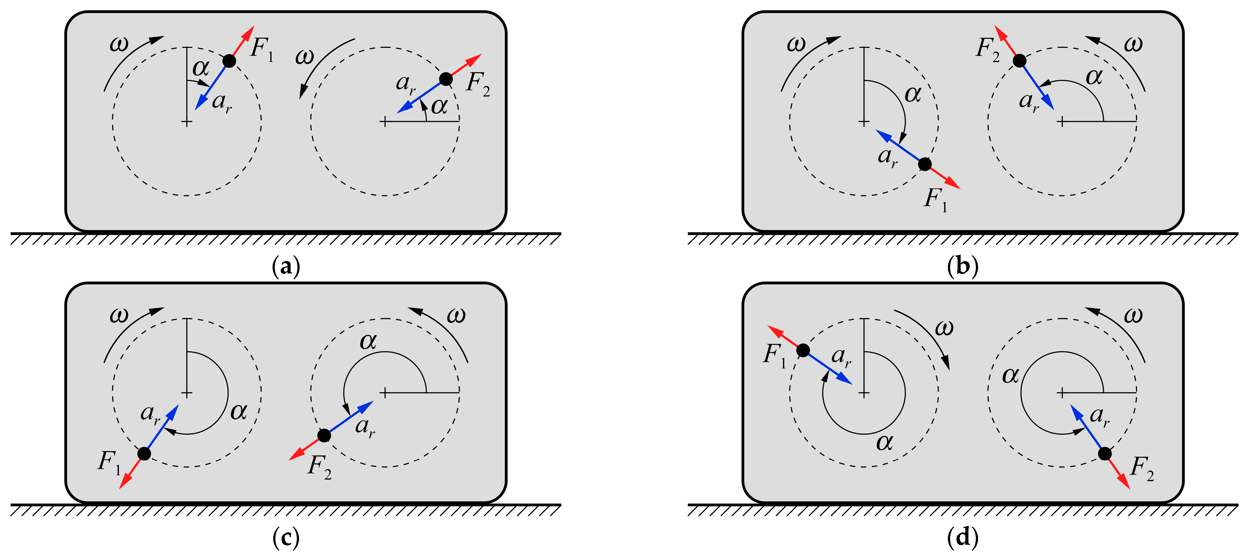
Assume that rightward motion of the mechanical system is the desired one. A positive (upward) component F_y reduces both the load on the ground and the friction force, which facilitates moving the robot. The opposite effect is caused by negative (downward) F_y that weighs down the system. When the horizontal component F_x is positive (rightward), it can be regarded as the propelling force that may excite forward motion of the robot, if only this force overcomes friction. Negative (leftward) F_x, in turn, may brake the system or even move it back. Different configurations of the internal masses together with forces F₁ and F₂ are shown in Figure 2. The coexistence of positive F_x and positive F_y (the phase of easier forward motion), as well as negative F_x and negative F_y (the rest phase, no backward motion), is particularly advantageous for efficient motion of the robot.

Let x(t) denote the displacement of the box as a function of time t. The horizontal motion and the static equilibrium in the vertical direction are described by

$$\left(M+2m\right)\ddot{x}=F_x-T,$$

(3a)

$$-\left(M+2m\right)g+F_y+N=0,$$

(3b)

where T is the friction force, N is the normal reaction of the ground, and g is the acceleration due to gravity. According to the classical Coulomb’s law of friction,

$$T=\mu N \mathrm{s}\mathrm{g}\mathrm{n}\left(\dot{x}\right).$$

(4)

Determining N from Equation (3b), taking into account Equation (2), and putting α = ωt, we obtain the following equation of motion:

$$\left(M+2m\right)\ddot{x}=mr{\omega }^2\left[\sin \left(\omega t\right)+\cos \left(\omega t\right)\right]\left[1+\mu \mathrm{s}\mathrm{g}\mathrm{n}\left(\dot{x}\right)\right]-\mu \left(M+2m\right)g \mathrm{s}\mathrm{g}\mathrm{n}\left(\dot{x}\right).$$

(5)

For the generality and convenience of further analysis, we introduce the dimensionless time and displacement, as follows:

$$\tau ={\omega }_{0}t, {\omega }_0=\sqrt{{\displaystyle \frac{g}{r}}}, X={\displaystyle \frac{x}{r}}.$$

(6)

Now, the non-dimensional counterpart of Equation (5) has the form

$$\ddot{X}={\displaystyle \frac{\beta {\mathsf{\Omega }}^2}{1+2\beta }}\left[\sin \left(\mathsf{\Omega }\mathsf{\tau }\right)+\cos \left(\mathsf{\Omega }\mathsf{\tau }\right)\right]\left[1+\mu \mathrm{s}\mathrm{g}\mathrm{n}\left(\dot{X}\right)\right]-\mu \mathrm{s}\mathrm{g}\mathrm{n}\left(\dot{X}\right),$$

(7)

where the overdots denote differentiation with respect to τ and the new dimensionless parameters are the relative angular speed Ω = ω/ω₀ of the particles and their relative mass β = m/M.

It should be noticed that the short Formula (4) for the friction force is reduced to the purely kinetic case: it is valid for the slip phase of motion ($\left|\dot{x}\right|\ne 0$), but it does not include the stick phase ($\left|\dot{x}\right|=0$). However, this simplified form of Coulomb damping is often used in both analytical and numerical studies in the fields of vibration and nonlinear dynamics (e.g., see [18,19]).

3. Analytical Studies of the System

In order to present the results, it is necessary to assume some values of the system parameters. In the computational studies of the considered system, the following values of the model parameters are treated as the basic dataset:

$$r=0.2 \left[\mathrm{m}\right], \mu =0.4, \beta =0.3, \mathsf{\Omega }=1.7.$$

(8)

These sample values ensure the robot’s movement. In the further part of the paper, a detailed qualitative and quantitative analysis of the robot’s behaviour for different values of particular parameters is presented.

Let us start with the determination of conditions for motion of the robot. First of all, the propelling force F_x must exceed the friction force. More precisely, we require F_x > T_max, where T_max = μNsgn(F_x) is the maximum force of static friction. In the non-dimensional formulation, the corresponding quantities are given as follows:

$${\widehat{F}}_X=\beta {\mathsf{\Omega }}^2\left[\sin \left(\mathsf{\alpha }\right)+\cos \left(\mathsf{\alpha }\right)\right],$$

(9a)

$$\widehat{N}=1+2\beta -\beta {\mathsf{\Omega }}^2\left[\sin \left(\mathsf{\alpha }\right)+\cos \left(\mathsf{\alpha }\right)\right],$$

(9b)

$${\widehat{T}}_{\mathrm{m}\mathrm{a}\mathrm{x}}=\mu \widehat{N}\mathrm{s}\mathrm{g}\mathrm{n}\left({\widehat{F}}_X\right).$$

(9c)

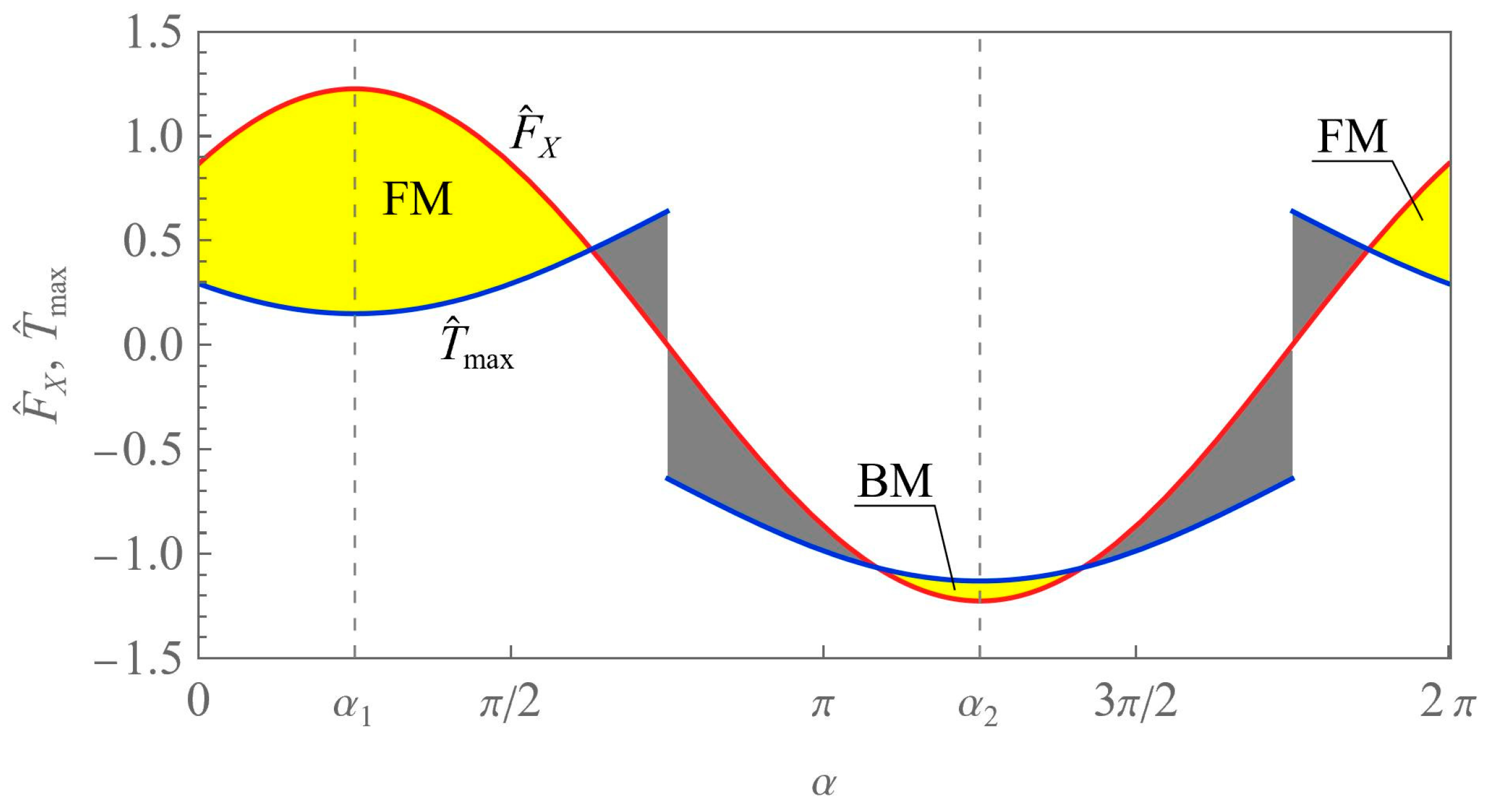
The first and the third force as the functions of angle α are presented in Figure 3. The shaded areas in the plot correspond to two phases of the robot dynamics: the active phase (yellow regions), and the rest phase (grey regions). The active phase includes both the desired forward motion (FM) and the undesired backward motion (BM). The latter one could be eliminated, for example, by decreasing the speed Ω. However, it would flatten the curve ${\widehat{F}}_X\left(\alpha \right)$ and reduce the active phase too.

Extrema of the propelling force occur at ${\alpha }_1=\pi /4$ (maximum) and ${\alpha }_2=5\pi /4$ (minimum). In order to ensure that the system moves forward without the return phase, we consider the conditions

$${\widehat{F}}_X\left({\alpha }_1\right)>{\widehat{T}}_{\mathrm{m}\mathrm{a}\mathrm{x}}\left({\alpha }_1\right), {\widehat{F}}_X\left({\alpha }_2\right)>{\widehat{T}}_{\mathrm{m}\mathrm{a}\mathrm{x}}\left({\alpha }_2\right)$$

(10)

that lead to the conclusions that Ω₁ < Ω < Ω₂ with

$${\mathsf{\Omega }}_1=\sqrt{{\displaystyle \frac{\mu (1+2\beta )}{\sqrt{2}(1+\mu )\beta }}}, {\mathsf{\Omega }}_2=\sqrt{{\displaystyle \frac{\mu (1+2\beta )}{\sqrt{2}(1-\mu )\beta }}}.$$

(11)

Moreover, the maximal allowed angular speed can be determined based on the restriction that the box should not lift off the ground, which means that the normal reaction (9b) must be positive. This condition leads to Ω < Ω_max with

$${\mathsf{\Omega }}_{\mathrm{m}\mathrm{a}\mathrm{x}}=\sqrt{{\displaystyle \frac{1+2\beta }{\sqrt{2}\beta }}}.$$

(12)

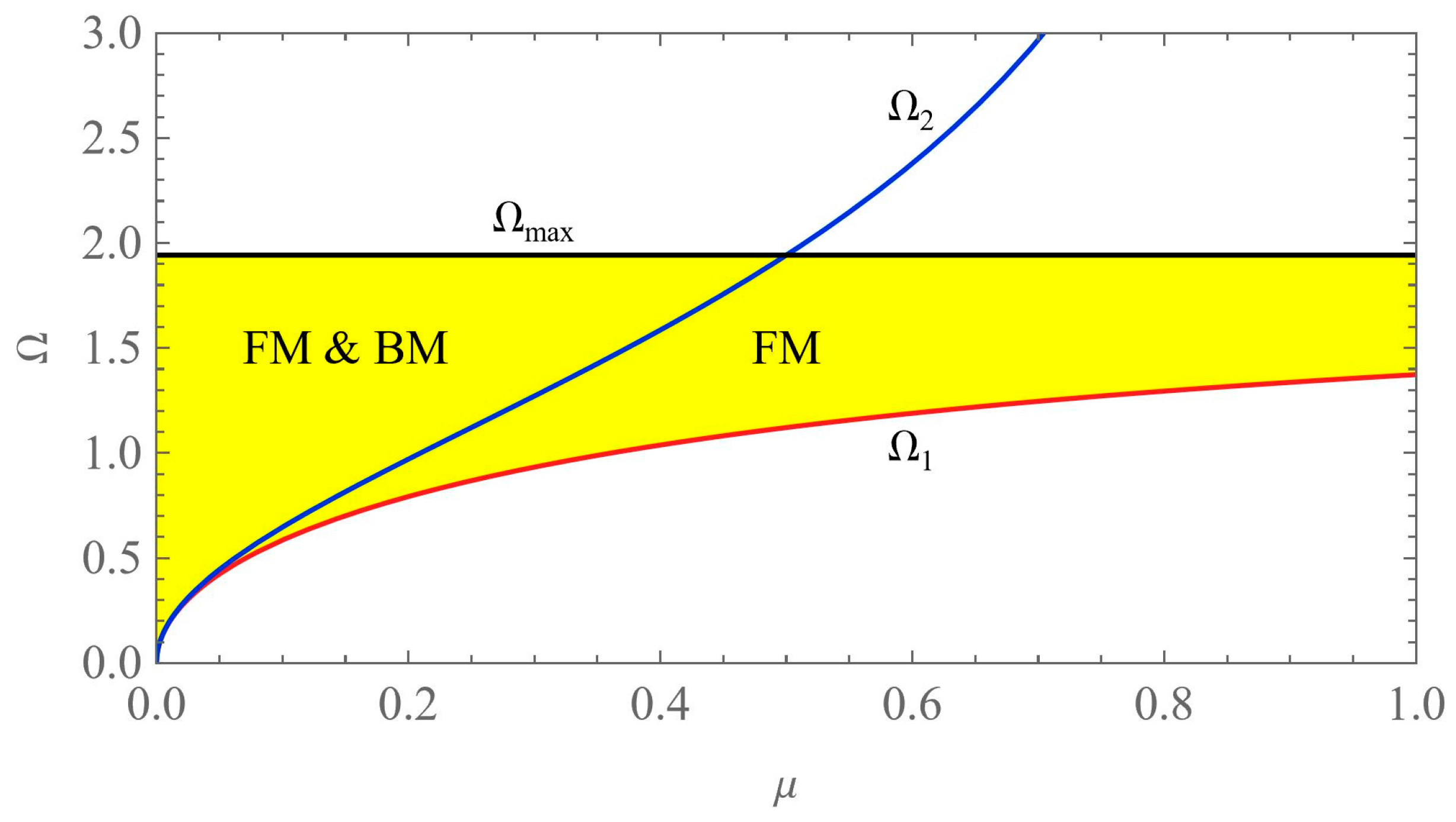
For dataset (8), the angular speed limits are Ω₁ ≈ 1.04, Ω₂ ≈ 1.59, and Ω_max ≈ 1.94. The three characteristic speeds as functions of the friction coefficient are shown in Figure 4. The shaded area (Ω₁ < Ω < Ω_max) indicates the working region of the robot. The curves Ω₂(μ) and Ω_max(μ) intersect exactly at μ = 1/2 for all values of β. Although Ω₂ tends towards infinity as μ tends to 1, the condition Ω < Ω_max is more restrictive for μ > 1/2. Ultimately, backward motion is eliminated if Ω₁ < Ω < min(Ω₂, Ω_max).

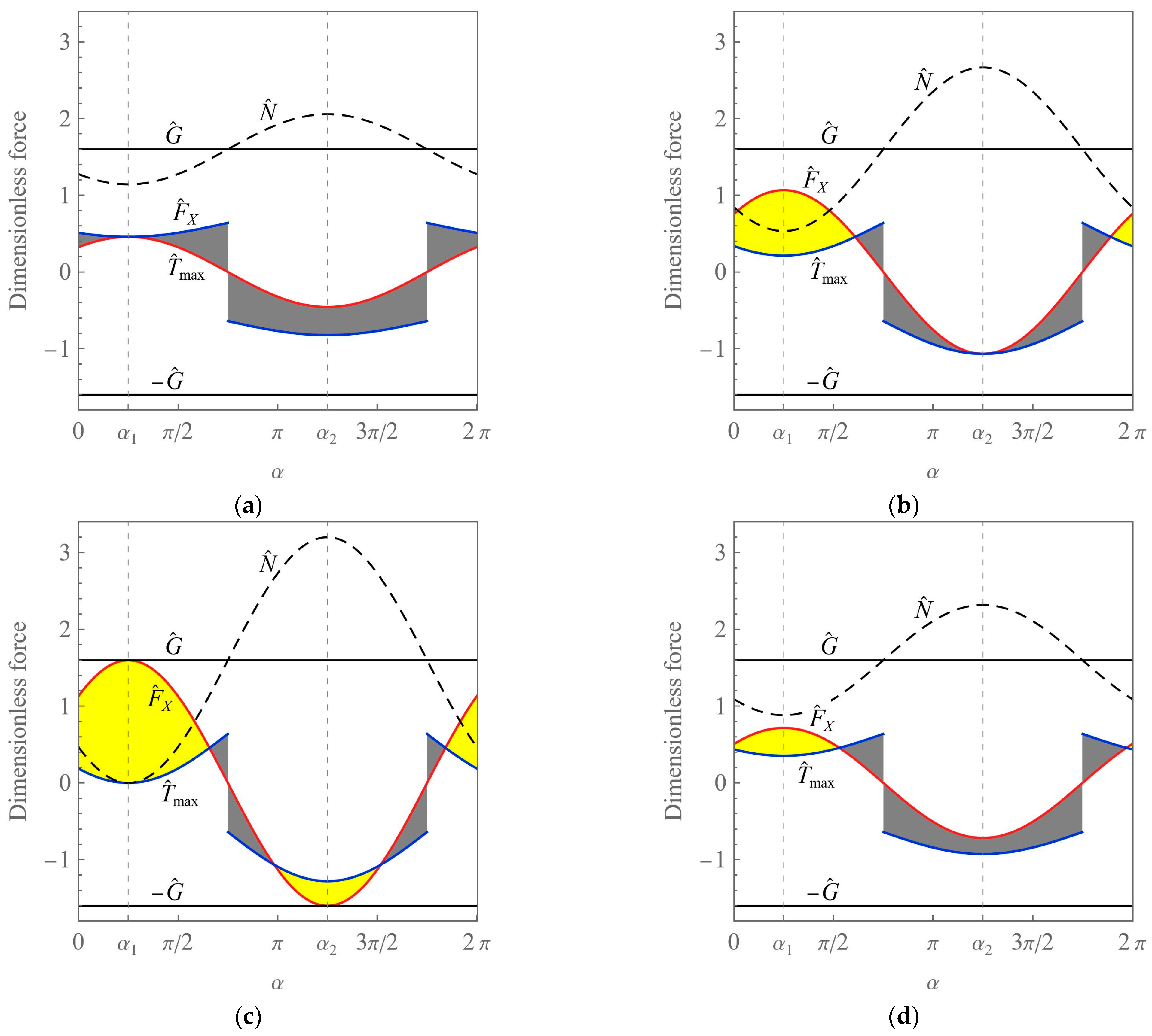
Figure 5 contains graphs of the non-dimensional forces for various values of the angular speed, including the characteristic ones. Apart from the quantities ${\widehat{F}}_X$ and ${\widehat{T}}_{\mathrm{m}\mathrm{a}\mathrm{x}}$, the normal reaction $\widehat{N}$ and the dimensionless total weight $\widehat{G}=1+2\beta$ are plotted. For ease of comparison, all the graphs have equal axis scales. When Ω = Ω₁, the whole range of α is occupied by the rest phase; thus, the system does not move at all (see Figure 5a). A significant reduction in the rest zone and the presence of the active phase without backward motion can be observed for Ω = Ω₂ (see Figure 5b). The active phase can be maximally extended in the extreme case when Ω = Ω_max, but the disadvantage is that the region of the undesired backward motion arises (see Figure 5c). Additionally, the intermediate case for Ω₁ < Ω < Ω₂ (here Ω = 1.3) is presented with a relatively narrow active zone and a relatively extended region of the rest phase (see Figure 5d).

It should be noticed that in the basic dataset (8), the friction coefficient μ < 1/2. For values μ > 1/2, the extreme case (Ω = Ω_max) looks different: the rest zone is more expanded because the backward motion does not occur at all (see Figure 4).

Time histories of the box displacement and velocity corresponding to different regions indicated in Figure 3, Figure 4 and Figure 5, and more extensive studies of the system are thoroughly discussed in the next section based on series of numerical ex-periments.

4. Numerical Studies of the System

The dynamical system described by Equation (7) is discontinuous due to the friction model. Unfortunately, this feature is the source of numerical difficulties during the time integration of ordinary differential equations (ODEs). To overcome this problem, we apply a simple smoothing technique that was discussed, for example, in [20,21]. Consider the dimensionless counterpart of the friction force (4):

$$\widehat{T}\left(V\right)=\mu \widehat{N} \mathrm{s}\mathrm{g}\mathrm{n}\left(V\right),$$

(13)

where $V=\dot{X}$. This discontinuous function can be replaced with a smooth approximation of the following form [20,21]:

$${\widehat{T}}_1\left(V\right)={\displaystyle \frac{2}{\pi }}\mu \widehat{N} \mathrm{a}\mathrm{r}\mathrm{c}\mathrm{t}\mathrm{a}\mathrm{n}\left(\eta V\right),$$

(14)

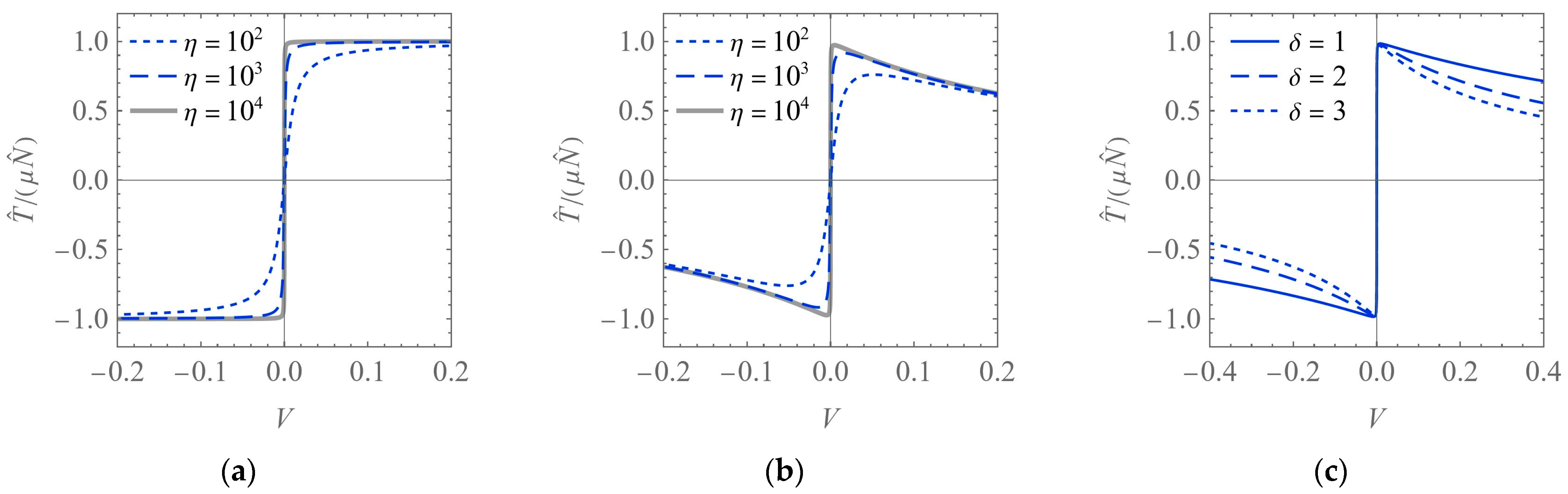
where η is the accuracy parameter (or steepness parameter). Such smoothed friction characteristics for different values of η are shown in Figure 6a. As can be seen, the larger the value of the parameter, the better approximation of Equation (13) and the steeper slope at V = 0.

Obviously, the classical Coulomb model is a considerable idealization, i.e., it assumes that the force of kinetic friction (in absolute value) is constant and equal to the maximum static friction force. More realistic approaches reflect the Stribeck effect, which consists in a decrease in the kinetic friction force (in absolute value) with increasing |V|. In such a case, the idealized law Equation (13) should be replaced, for example, with the following smoothed model [20,21]:

$${\widehat{T}}_2\left(V\right)={\displaystyle \frac{2}{\pi }}·{\displaystyle \frac{\mu \widehat{N}}{1+\delta \left|V\right|}} \mathrm{a}\mathrm{r}\mathrm{c}\mathrm{t}\mathrm{a}\mathrm{n}\left(\eta V\right),$$

(15)

where the new parameter δ is a positive number that affects the rate of decrease in the kinetic friction force. Friction characteristics of this type for various values of η and δ are depicted in Figure 6b,c.

It should be emphasized that models Equations (14) and (15) work well for the slip phase of motion (|V| > 0), while in the stick phase (|V| = 0), the friction force becomes zero. This is the main drawback of the basic smoothing approach. However, for the sake of clarity, the preliminary dynamic studies illustrating the robot’s concept have been conducted using this simplification.

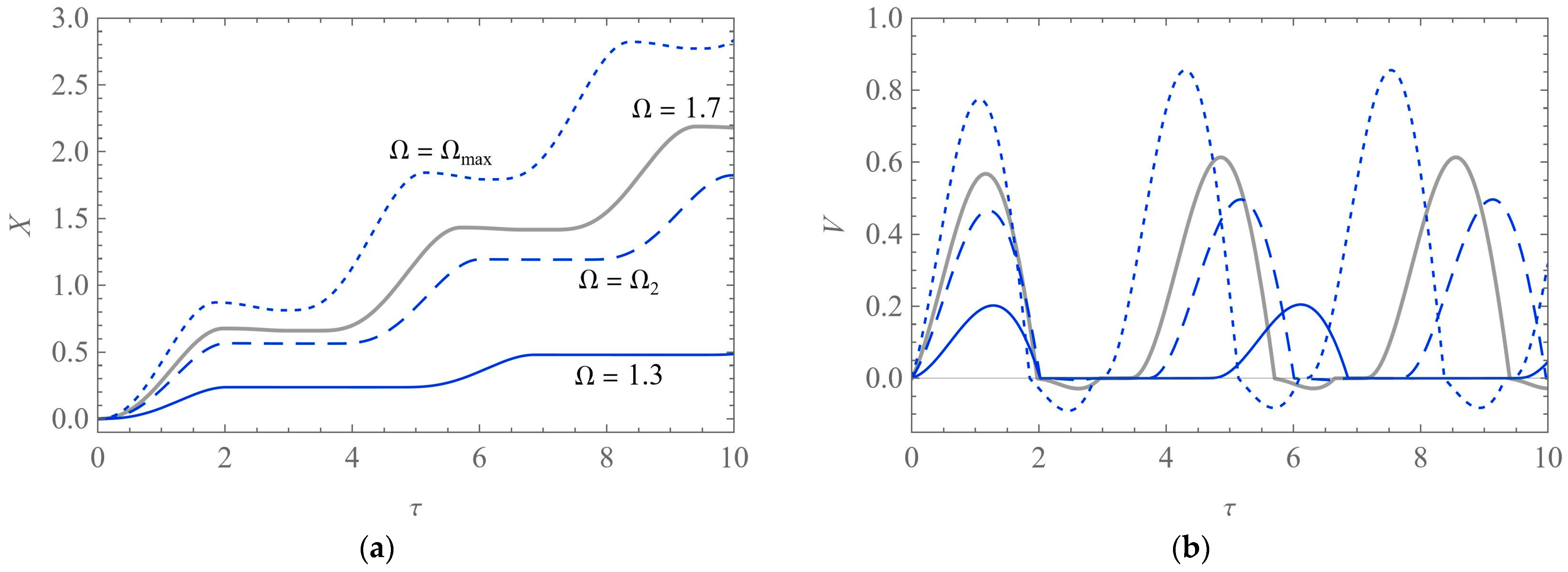
Let us start with numerical solutions computed using the Coulomb friction model smoothed with η = 10⁴. The results have been obtained for the basic dataset with varying Ω and for zero initial conditions: X(0) = V(0) = 0. The time histories of X and V are presented in Figure 7. Three solutions (blue lines: solid, dashed, and dotted) illustrate the cases shown in Figure 5b–d, whereas the basic solution (solid grey) is connected with Figure 3. Hence, the active phase including both forward motion (V > 0) and backward motion (V < 0) occurs only for high values of the angular speed (Ω = Ω_max and Ω = 1.7). The rest phase, in turn, is indicated by the intervals of constant position and zero velocity.

The steady-state motion of the system is achieved after several periods of the excitation, that is, for τ > kτ_p, where τ_p = 2π/Ω and k is a small natural number. In the cases shown in Figure 7, we can estimate that k = 2. Evidently, the differences between the ranges of functions X(τ) and V(τ) for various values of Ω are significant. For comparison purposes, we can estimate the total displacement per period and the average velocity per period:

$$X_p=X\left((k+1){\tau }_p\right)-X\left(k{\tau }_p\right), V_p={\displaystyle \frac{X_p}{{\tau }_p}}.$$

(16)

when dealing with different combinations of model parameters, the value of k may be increased (e.g., k = 5 or k = 10) to ensure that the transient response of the system is omitted. For the analyzed solutions, the results are given in

Table 1. The total displacement per period and the average velocity per period evaluated for the numerical solutions shown in Figure 7.

Ω	τp	Xp	Vp
1.30	4.83	0.242	0.050
1.59	3.96	0.629	0.159
1.70	3.70	0.756	0.205
1.94	3.24	0.979	0.303

. The displacement and velocity increase nearly linearly with the angular speed.

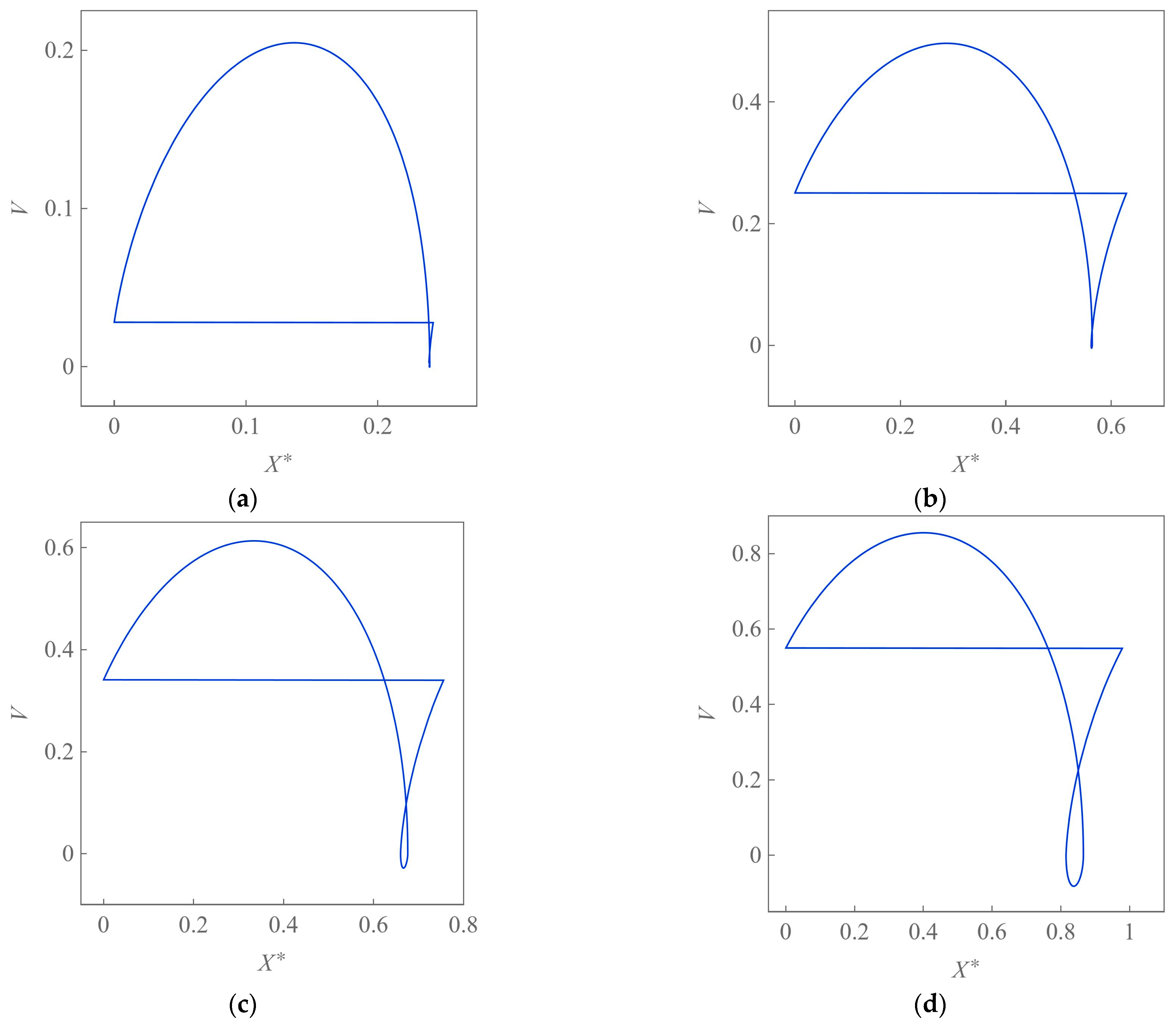
Figure 8 contains the phase portraits for these four cases. More precisely, the steady motion of the system is illustrated on the plane (X*, V) with X* = mod(X, X_p). Thus, the horizontal ranges of the curves are equal just to X_p. The horizontal segments result from the specific definition of X*. The loops near V = 0, in turn, are related to backward motion of the robot. The time histories presented in Figure 7 indicates that a stick–slip motion appears for $\mathsf{\Omega }<{\mathsf{\Omega }}_2$. This looks similar to the self-induced oscillations, although the physics of the phenomenon is different.

In order to gain a deeper insight into the effect of various parameters on the total displacement and average velocity per period, series of dynamic simulations have been conducted for numerous datasets.

Table 2. Ranges and step sizes for the dimensionless model parameters used in the numerical studies.

Parameter	Symbol	Range	Step
Friction coefficient	μ	〈0.02, 1〉	0.01
Relative mass of the particles	β	〈0.05, 1.5〉	0.05
Relative angular speed	Ω	〈0.5, 2.5〉	0.05

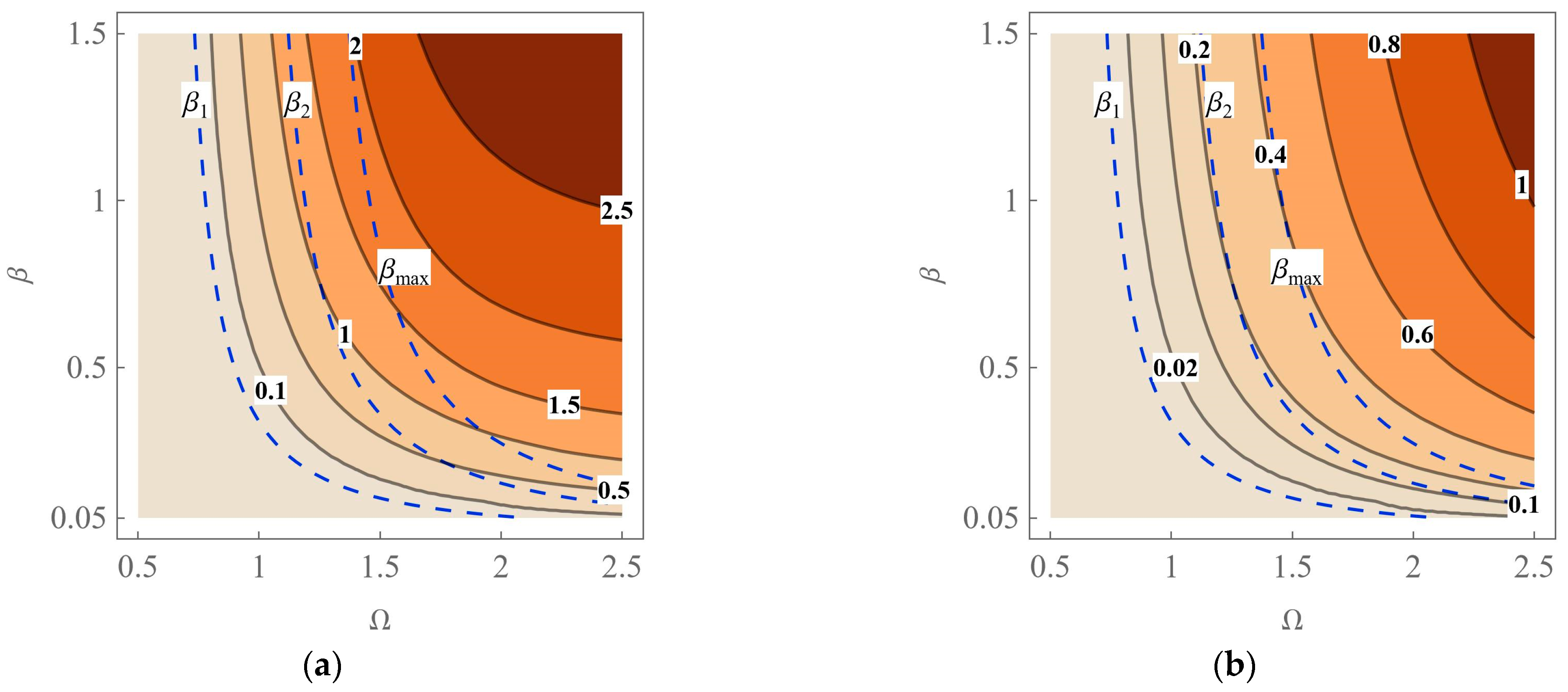
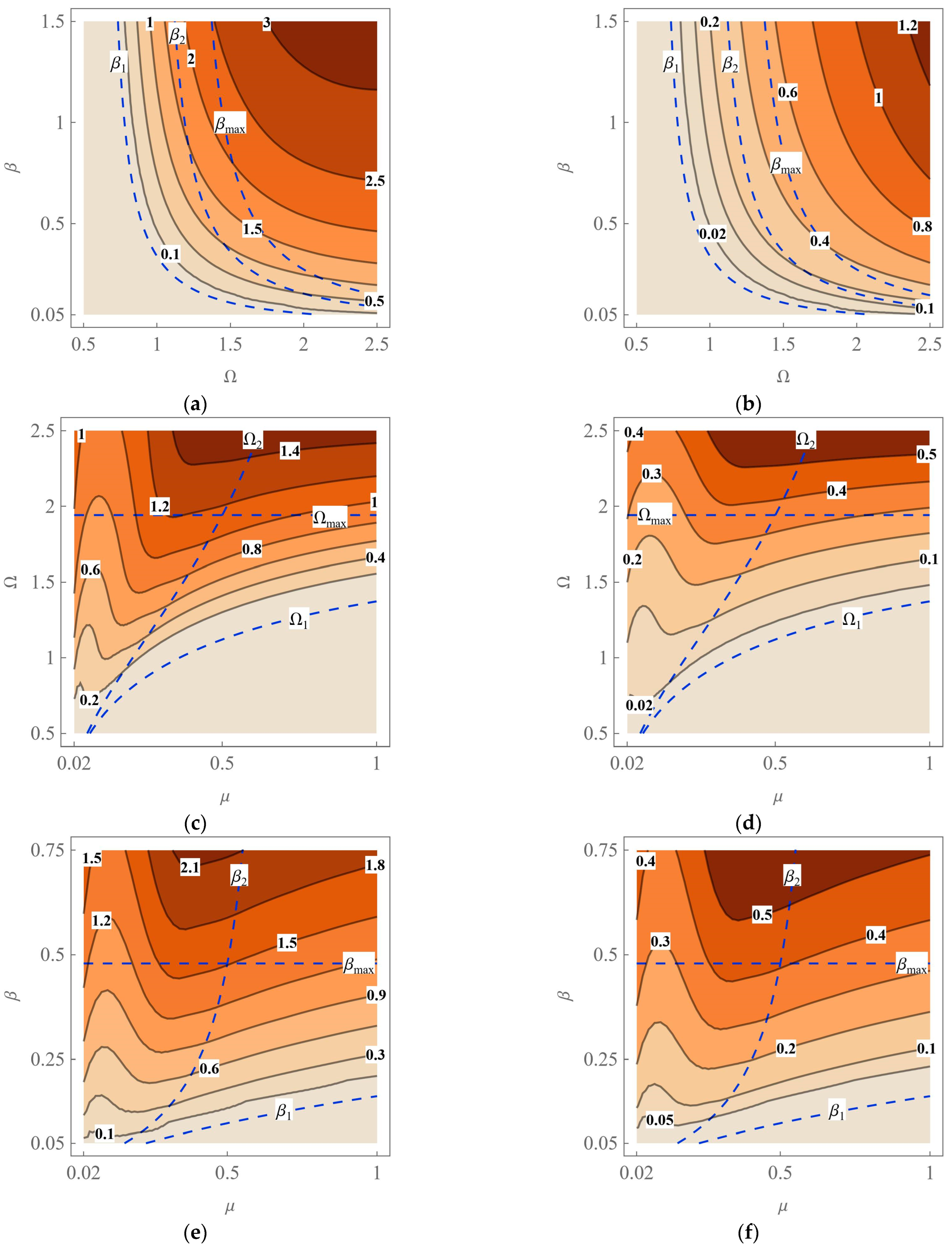
contains the ranges and step sizes of particular parameters varied. All numerical solutions have been analyzed with k = 5 to estimate X_p and V_p. The resulting filled contour plots on particular parameter planes are presented in Figure 9.

As results from the maps, the three considered parameters can have a significant effect on the displacement and velocity. It may seem, for example, that for a given value of μ we can choose a new value of Ω or β to obtain two or three times larger X_p or V_p when compared to the results in Table 1. However, the working regions of the mechanical system are restricted by the conditions for motion. These constraints are indicated by the dashed lines and curves overlaid on the maps. On the plane (μ, Ω), one can see the three limit functions derived analytically: Ω₁(μ, β), Ω₂(μ, β), and Ω_max(β). Hence, the applicability of the contour plots in Figure 8c,d is limited to the region filled with yellow in Figure 4. When it comes to the planes (Ω, β) and (μ, β), the corresponding limits of β are visible: β₁(μ, Ω), β₂(μ, Ω), and β_max(Ω). Consequently, in Figure 9a,b,e,f, we should focus on the subregions bounded by the curves/lines labelled as β₁ and β_max.

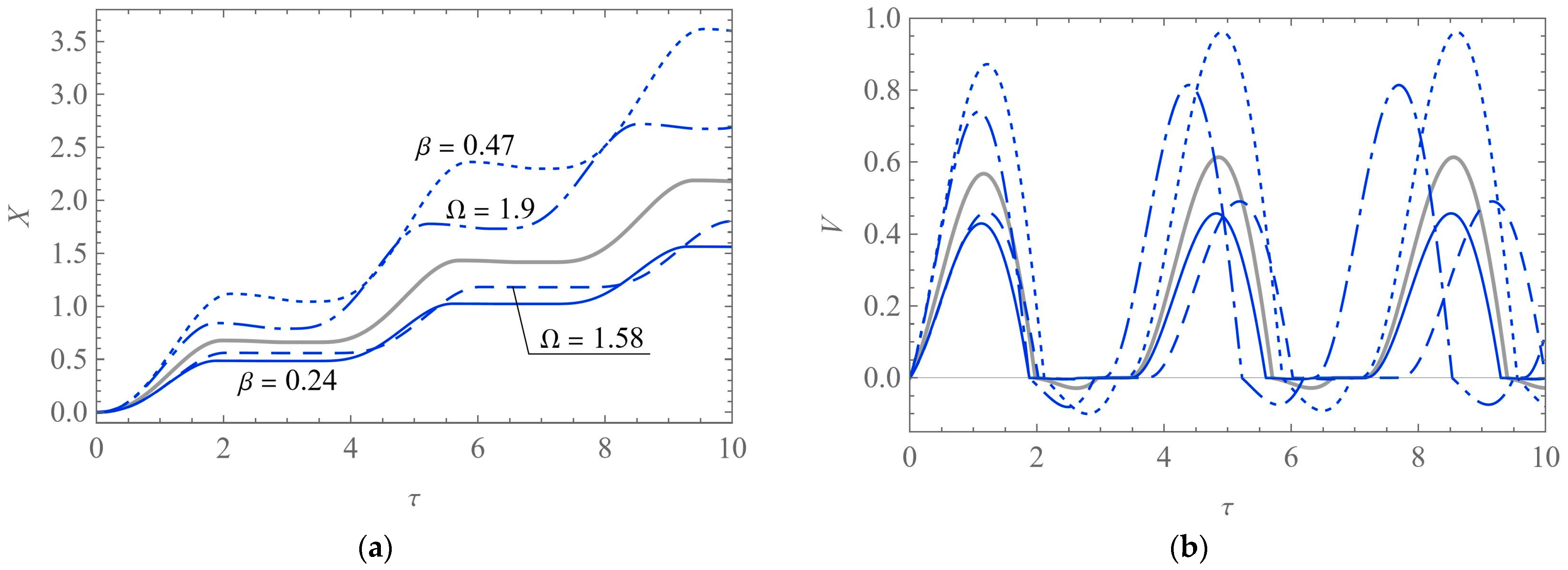
Figure 10 contains the time histories X(τ) and V(τ) obtained for modified values of selected parameters. As can be seen, the basic solution (solid grey) can be compared to the cases when Ω (dashed blue and dash-dotted blue) or β (solid blue and dotted blue) is varied. Although the active phase includes the return effect (rather weak), the near maximal values of the parameters (Ω_max ≈ 1.94, β_max ≈ 0.48) result in greater ranges of motion per period, as well as higher average velocities of the system: X_p ≈ 0.943, V_p ≈ 0.285 and X_p ≈ 1.255, V_p ≈ 0.339, respectively. Thus, a change in the relative mass can give a better improvement in X_p and V_p than a change in the angular speed. For the lower values of Ω and β (close to Ω₂ ≈ 1.59 and β₂ ≈ 0.24), in turn, there is no backward motion, but the displacements and velocities are lower too: X_p ≈ 0.622, V_p ≈ 0.156 and X_p ≈ 0.539, V_p ≈ 0.146, respectively.

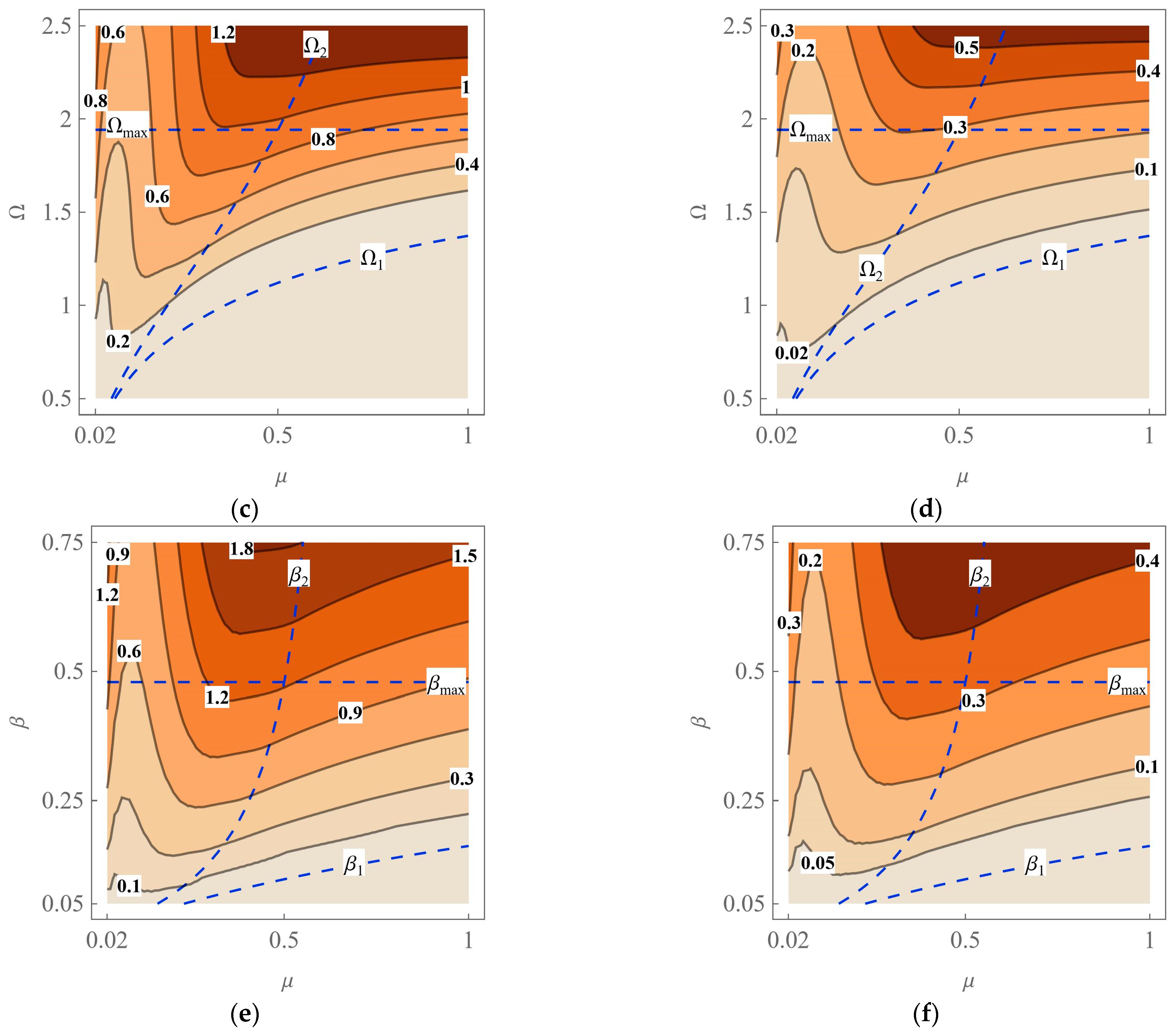
A similar parametric analysis can be performed for the Stribeck model of friction. The results reported below have been obtained for δ = 2 and η = 10⁴. This time, let us start with the maps shown in Figure 11. The dependencies of X_p and V_p on particular pairs of parameters are of a similar nature, as in Figure 9. However, a careful comparison reveals that now the two quantities reach values higher by about 25% in the subregions bounded by the triples of the limit functions, i.e., Ω₁, Ω₂, and Ω_max or β₁, β₂, and β_max. As could be supposed, the decrease in the resistance to motion due to the Stribeck effect allows for the system to move more efficiently.

By analogy to Figure 7a, the time histories X(τ) obtained for selected values of the angular speed are shown in Figure 12a. When it comes to the modifications based on the discussed contour plots, the solutions are presented in Figure 12b that may be compared to Figure 10a. As before, the results exhibit the active phase of the robot with no backward motion when Ω ≤ Ω₂ or β ≤ β₂. However, the cases with Ω₂ < Ω ≤ Ω_max or β₂ < β ≤ β_max may be treated as more beneficial despite the minor return effect.

In order to more precisely confront the results related to the different friction models, we focused on just the effect of the angular speed on the total displacement per period and the average velocity. Figure 13 includes a straightforward comparison of the data given in Table 1 (the Coulomb model, i.e., δ = 0) and the analogous results obtained for the Stribeck model with δ ∈ {1, 2, 3}. Let us treat X_p(Ω) and V_p(Ω) for the Coulomb model as the reference values. When comparing the displacements and velocities in the cases with δ = 2 and δ = 0, for example, the relative differences vary from about 50% for Ω = 1.3 to about 20% for Ω ≈ 1.94. Certainly, the occurrence of the Stribeck effect in the friction characteristics plays a positive role in the improvement of the robot performance. Values of X_p(Ω) and V_p(Ω) increase with parameter δ.

In the end, it is important to notice that the dynamics of the mechanical system depends on the initial conditions. In the reported simulations, we employed the zero conditions only, i.e., X(0) = X₀ and V(0) = V₀ with X₀ = V₀ = 0. Similarly, the angle of rotation could be defined as α = α₀ + ωt = α₀ + Ωτ, where α₀ denotes the initial value; we have taken α₀ = 0. Both V₀ and α₀ are crucial for initiating motion of the robot. However, this problem, together with the physical realization of the inertial drive, goes beyond the scope of this study. Thus, the numerical experiments have been focused rather on the steady-state motion of the system.

5. Conclusions

The primary goal of this paper has been achieved. We have shown that the motion of a capsule system on a rough horizontal plane caused only by the rotation of two internal masses is possible.

The mathematical model of the robot has been presented, and the working region of the system has been specified in terms of the model parameters. There are three characteristic values of angular velocities which define areas of qualitatively different robot movements (see Figure 4). To illustrate the idea of the inertial drive and the interplay between particular parameters, extensive numerical studies have been conducted for two models of friction.

The numerical solutions to the dynamic problem have been analyzed with regard to the total displacement per period and the average velocity per period. The related maps on particular parameter planes allow for controlling the robot performance described by these two indicators. The quantitative analysis of the influence of three factors on the motion has been presented graphically (Figure 7, Figure 8, Figure 9, Figure 10, Figure 11, Figure 12 and Figure 13). The analysis indicates that generally the displacement and velocity increase with the increase in dimensionless mass of the rotating points and with the increase in their angular velocity. The situation is different in the case of the coefficient of friction. Its increase causes a decrease in the displacement and average speed of the robot. It is worth noting that too low a value of μ will result in an unfavourable reverse movement (see Figure 9c–f and Figure 11c–f). Moreover, the more realistic friction model that includes the Stribeck effect turns out to be advantageous for efficient motion of the system when compared to the basic Coulomb model.

It should be emphasized that the present study has not focused on detailed practical issues, such as the shape of the capsule, the physical realization of the inertial drive, or the power supply. For example, in a real system, the internal masses could be revolved around a common axis, which should reduce the tendency of the inertial forces to rotate and lift the box. This particular problem and many others will be considered in further steps, leading to the experimental validation of the theoretical results.