Abstract
The aging of power plant pipelines has led to significant leaks worldwide, causing environmental damage, human safety risks, and economic losses. Rapid leak detection is critical for mitigating these issues, but challenges such as varying leak characteristics, ambient noise, and limited real-world data complicate their accurate detection and model development. To address these issues, we propose a leak detection model that integrates stepwise transfer learning and an attention mechanism. The proposed model utilizes a two-stage deep learning process. In Stage 1, one-dimensional convolutional neural networks (1D CNNs) are pre-trained to extract root mean square (RMS) and frequency-domain features from acoustic signals. In Stage 2, the classifier layers of the pre-trained models are removed, and the extracted features are fused and processed using a bidirectional long short-term memory (LSTM) network. An attention mechanism is incorporated within the LSTM to prioritize critical features, enhancing the ability of the model to distinguish leak signals from noise. The model achieved an accuracy of 99.99%, significantly outperforming the traditional methods considered in this study. By effectively addressing noise interference and data scarcity, this robust approach demonstrates its potential to enhance safety, reduce risks, and improve cost efficiency in industrial pipelines and critical infrastructure.
1. Introduction
The aging of power plant piping, both domestically and internationally, has increasingly resulted in severe leaks, causing substantial harm to human safety, the environment, and economic stability [1,2,3]. Consequently, the prompt identification of leaks in aging piping systems is important for ensuring safety and economic efficiency [4,5,6]. Historically, various sensors, including acoustic, vibration, pressure, and ultrasonic types, have been explored for early leak detection [7,8,9]. However, accurately detecting leaks remains challenging due to the varying physical characteristics of leaks, which are influenced by factors such as pressure, material properties, and environmental conditions. Ambient noise, in particular, significantly complicates the differentiation of leak signals, leading to reduced detection rates [10,11].
With the advent of large-scale data, advancements in deep learning (DL) and machine learning (ML) technologies have progressed rapidly, enabling solutions to a range of complex problems [12,13,14]. These technologies have become integral in industrial applications, excelling in modeling complex patterns and delivering accurate predictions [15,16,17]. Artificial intelligence (AI), in particular, has emerged as a transformative tool for enhancing productivity, reducing costs, and improving safety across various sectors, owing to its advanced learning and inference capabilities [18,19,20]. This has raised significant expectations for the role of AI in detecting minor leaks in aging piping systems, fostering active research in this area [21,22,23]. For instance, Mysorewala et al. achieved 93% accuracy in detecting vibrations caused by leaks using low-power accelerometers and a support vector machine (SVM) model [24]. Similarly, Ahmad et al. reported detection performances of 98.4% and 96.67% using convolutional autoencoders and convolutional neural network (CNN) models, respectively [25]. These studies demonstrate the potential of AI to advance fine leak detection in aging piping systems.
Despite these advancements, existing methods face significant limitations. Traditional signal processing techniques often fail to accurately distinguish leak signals from noise, as noise can distort the defining characteristics of leak signals. Additionally, achieving high accuracy and performance in leak detection requires extensive data, yet collecting leak data in real-world environments is both challenging and hazardous. Even under controlled conditions that simulate real-world scenarios, the data collected are often insufficient due to the limitations of the experimental setup. Therefore, there is an urgent need for research focused on differentiating leak signals from noise with high accuracy and reliability, even when working with small datasets.
To address these challenges, this paper proposes a feature fusion DL model based on stepwise transfer learning (TL) [26,27,28] that utilizes an attention mechanism. Time-domain root mean square (RMS) and frequency-domain frequency patterns are generated from one-dimensional (1D) time-series acoustic signals acquired using multiple acoustic sensors. These patterns are then used to train the feature fusion model based on TL. The proposed model comprises a two-stage process (Stages 1 and 2). In Stage 1, key features are extracted from RMS and frequency pattern signals using 1D CNN models for each domain after preprocessing the source domain data. In Stage 2 of the TL process, the classifiers of the 1D CNN models trained in Stage 1 for each domain are removed, and the output features of these models are combined. The preprocessed RMS and frequency pattern signals from the target domain data are then input into a model enhanced with bidirectional long short-term memory (LSTM) [29].
The bidirectional LSTM captures both forward and backward temporal dependencies, enriching the understanding of the model of sequence data. Unlike unidirectional LSTMs, which process input sequences in a single direction from past to future, bidirectional LSTMs consider the entire context of the data, thereby improving the detection of subtle patterns and the prediction accuracy. Numerous studies have demonstrated that bidirectional LSTMs often outperform unidirectional LSTMs in tasks requiring temporal feature extraction due to their ability to capture more comprehensive temporal dependencies [30,31,32]. By processing sequence information in both directions simultaneously, the bidirectional LSTM enables the model to utilize richer contextual information. Additionally, a dot-product-based attention mechanism [33] applied to the LSTM in each direction helps the model focus on important patterns in the input from both directions, effectively extracting fused sequence features in the time and frequency domains. Subsequently, the outputs of these attention layers are concatenated into a single layer. Finally, a classifier is added to this combined layer to extract domain-specific features and make the final prediction. This approach allows the model to achieve more accurate predictions by leveraging attended features extracted from both directions of the input.
This paper is organized as follows: In Section 1, the research background is discussed, emphasizing the significance of addressing leak issues in aging pipes. Section 2 outlines the process of feature extraction in the RMS and frequency domains, along with the data preprocessing techniques applied. Section 3 introduces the proposed feature fusion leak detection model, which integrates TL and bidirectional attention mechanisms. Section 4 describes the data collection setup and assesses the performance of the model. Finally, Section 5 provides a conclusion and suggests potential avenues for future research.
2. Data Preprocessing for Feature Extraction
This section describes the data preprocessing methods used to differentiate between leak and normal states based on 1D time-series acoustic signals obtained from several microphone sensors. As outlined in [34] and illustrated in Figure 1, 1D features representing RMS patterns and frequency patterns are extracted. At this stage, two signal processing techniques, designated as (), are applied to extract the RMS pattern features. The detailed nomenclature and description of the data preprocessing methods are provided in Table 1.
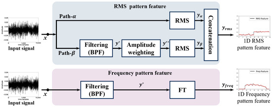
Figure 1.
Structure for RMS and frequency pattern extraction.

Table 1.
Nomenclature for data preprocessing.
First, in , the input data are sampled at intervals of without any filtering, and the sampled data are represented as . A moving average window is then applied to the sampled input data to calculate their RMS level. Through this process, is generated, where is calculated as shown in Equation (1):
where denotes a coefficient used to normalize the data and represents the window size for the RMS level calculation of the received data.
In , the preprocessed signal is first generated by passing the input data through a band-pass filter (BPF) block, as defined in Equation (2):
where the operates within the 20 kHz to 40 kHz frequency range, capturing ultrasonic leak signals primarily caused by turbulence at the leak site. This frequency range effectively reduces low-frequency mechanical noise, focusing on critical leak signal features to improve detection accuracy. Additional parameters, such as the amplitude weighting function and window size for RMS level calculation, are carefully selected to optimize signal processing. These parameters highlight key signal features, minimize irrelevant noise, and prepare the signal for subsequent processing stages. The preprocessed signal then passes through the “amplitude weighting block”, where a weighting function is applied in the frequency domain. This function emphasizes desired frequency components, suppresses external noise, and amplifies signals with concentrated spectral presence. The processed signal is calculated as shown in Equation (3):
where denotes the 1D Fourier transform (FT) and represents the 1D inverse FT.
The weighting function is defined as shown in Equation (4):
where and are the beginning and ending frequencies for the windowing operation, and represents the amplification ratio of the signal within this range. In the RMS block of , the RMS level for is calculated based on Equation (1), similar to , to generate . Finally, the and feature vectors from both paths are combined to produce the final RMS pattern feature .
Frequency pattern features are then derived from the received time-series data by analyzing the frequency response magnitude of the leak signal. Similar to of the RMS pattern features in Figure 1, the frequency pattern feature is obtained by converting the preprocessed signal , after passing through the BPF block, into frequency-domain data using the 1D FT, as shown in Equation (5):
This process results in the final frequency pattern feature .
Figure 2 provides a visual representation of the pattern features extracted from the RMS and frequency components of leak and noise signals. Figure 2a illustrates the RMS pattern features, with the -axis divided into two sections. The left side corresponds to RMS levels computed directly without filtering in , while the right side represents RMS levels calculated after filtering and amplitude weighting in . For the leak feature shown in Figure 2a, the RMS pattern exhibits an increasing trend in , whereas for the noise feature, external noise is effectively filtered, leading to a decreasing trend in the RMS pattern size. Figure 2b displays the frequency pattern.
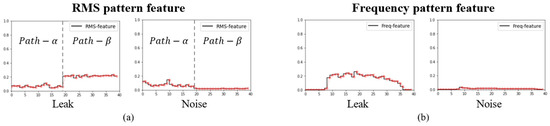
Figure 2.
Features of RMS and frequency patterns for leak and noise signals: (a) RMS pattern feature, (b) frequency pattern features, where the spectrum size and pattern of the leak signal, generated through BPF filtering, are clearly distinguishable from those of the noise signal.
The 1D RMS and frequency pattern features are further integrated with domain-specific features obtained from multiple sensors to train the proposed model. Figure 3 demonstrates the sequential alignment of these pattern features along the channel direction, using data gathered from four sensors to form two-dimensional (2D) tensor features. This method combines features from various sensors, structuring the resulting 2D tensor as input for the proposed model, as discussed in Section 3.
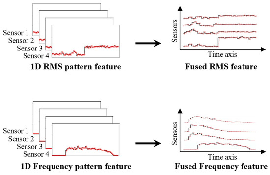
Figure 3.
Fusion of 1D pattern features using four sensors for model training.
3. Proposed Leak Detection Model
Using the data preprocessing methods for feature extraction described in Section 2, the 1D RMS and frequency-domain data were converted and utilized for training the proposed model for fine leak detection. The proposed model comprises two stages, as shown in Figure 4. TL is carried out by transferring the knowledge acquired in Stage 1 in (source domain) to Stage 2 (target domain). This approach utilizes the pre-trained model from Stage 1 to mitigate overfitting issues caused by the limited data available in the target domain.
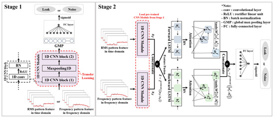
Figure 4.
Architecture of a feature fusion DL model based on stepwise TL using an attention mechanism.
In Stage 1, a 1D CNN structure is utilized to extract local feature maps from the preprocessed 1D RMS and frequency data, focusing on identifying fine leak or noise signals. The 1D convolution operation is mathematically defined in Equation (6):
where denotes the domain, with denoting the time domain and the frequency domain. denotes the 1D feature map of domain at layer , with dimensions . denotes the 1D feature map of domain at layer , whereas denotes the kernel function with a window size of , mapping from feature map of domain at layer to feature map at layer . The bias term is denoted by , and denotes the activation function. denotes the number of output feature maps at layer , denotes the total number of convolution layers in domain , and denotes the list of 1D feature maps at layer connected to feature map .
To pre-extract features for leak and noise signals, a 1D convolution layer with a kernel size of and eight filters is applied, as summarized in Table 2. This convolution operation is followed by batch normalization (BN) and MaxPooling1D, which compress the extracted features. This process corresponds to the 1D CNN block (1) within the 1D CNN module, forming the initial feature extraction phase for fine leak detection.
Table 2.
Detailed structure of single 1D CNN model for both time and frequency domains.
Next, a second 1D convolution layer with the same kernel size and 16 filters is applied, followed by BN and global max-pooling to extract the main representative features. This corresponds to the 1D CNN block (2) within the same module. The 1D convolution employs the rectified linear unit (ReLU) as its activation function. To enable independent learning for each domain, the final output feature map of domain is used as the input for a binary classifier. The first layer of this classifier contains eight neurons activated by a ReLU function, while the output layer includes a single neuron with a sigmoid activation function.
In Stage 2, the pre-trained “1D CNN Module” for each domain, independently learned and stored in Stage 1, is loaded, as shown in Figure 4. Feature fusion is performed by removing the classifiers from each model and combining the output feature maps and , representing the time and frequency domains, respectively, into a single higher-dimensional layer . This fusion process is mathematically defined in Equation (7) as follows:
where denotes the concatenation function, which merges the two feature maps. Through this feature fusion process, temporal- and frequency-domain information are integrated, resulting in richer features that capture more comprehensive insights.
A bidirectional LSTM network is then applied to the fused feature data. This network consists of a forward output with 128 units and a backward output with 128 units, which collectively consider sequence information in both forward and backward directions. BN is applied to the bidirectional LSTM outputs to stabilize the learning process. By leveraging the bidirectional LSTM, the model processes sequence data more effectively, utilizing context from both input directions.
To emphasize important information at each time step, a dot-product-based attention mechanism is applied to the outputs of each LSTM layer. The attention score is calculated using Equation (8) as follows:
where indicates the LSTM direction for forward and for backward, denotes the hidden state at time step , denotes the hidden state at all time steps , and represents the transpose of . A softmax operation is applied to the attention scores to normalize them into probabilities, which are then used to compute the attention weights. This process is defined in Equation (9) as follows:
where represents the attention weight between the hidden state at the current time step and the hidden state at a different time step. The softmax operation in Equation (4) converts each attention score into a probability value, enabling the calculation of weights for each time step. Additionally, denotes the summation index that includes all possible time steps, ensuring the denominator normalizes the total similarity scores into a probability distribution across the sequence.
The context vector is then computed as the weighted sum of the attention weight and the hidden state across each time step , as shown in the following Equation (10):
Using Equation (5), the hidden state at each time step is weighted by its corresponding attention weight to form the context vector . This allows the model to summarize and extract the most important information from the entire input sequence effectively.
Finally, the attention vector for each direction is calculated in Equation (11) by combining the context vector with the current hidden state , providing domain-specific trainable attention weights.
where denotes the learnable weight matrix for direction and denotes the concatenation of and . The hyperbolic tangent function (tanh) introduces non-linear transformation, generating the final attention vector and refining the focus of the model on domain-specific features.
Attention vectors and , obtained from the forward and backward directions of the bidirectional LSTM, are concatenated to form a single vector . This process is mathematically defined in Equation (12) as follows:
Subsequently, a fully connected (FC) layer comprising 64 units is added, with serving as the input. This layer employs a ReLU activation function to introduce non-linearity, enhancing the ability of the model to capture complex patterns in the fused features. The final output layer consists of a single neuron with a sigmoid activation function, designed to perform binary classification, distinguishing between leak and noise signals. The architecture of Stage 2 in the proposed feature fusion model, incorporating TL and the described layers, is summarized in Table 3. Additionally, the nomenclature for the proposed leak detection model is summarized in Table 4, which defines the key variables and their corresponding descriptions for clarity and reference.
Table 3.
Detailed structure of Stage 2 in the proposed leak detection model.
Table 4.
Nomenclature for the proposed leak detection model.
4. Experimental Results
4.1. Data Collection Environment and Experimental Setup for Leak Detection
This paper investigated the model transfer across different testbed environments. In Stage 1, the model was pre-trained using leak signals and mechanical noise data collected from a source domain within a controlled testbed environment, as shown in Figure 5 [34]. The dataset was obtained using four microphone acoustic sensors, each operating at a sampling frequency of 100 kHz, with a signal measurement duration of 1.5 s per recording. The commercial ICP microphone (Model HT378A06) from PCB Piezotronics, located in Depew, NY, USA, was utilized as the sensor for this study [22]. Leak signals were recorded at 100 distinct locations along the pipeline under 25 unique combinations of leak pressure and leak size. The leak pressure was varied from 1 bar to 5 bar in increments of 1 bar, while the leak diameter ranged from 0.5 mm to 2.5 mm, increasing in intervals of 0.5 mm.
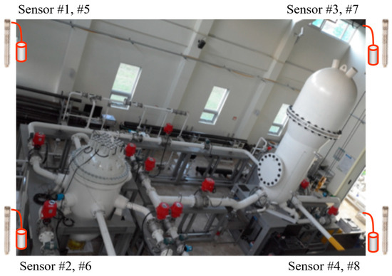
Figure 5.
Source domain data collection testbed environment using plant piping specimens.
In the target domain, data were collected from 10 leak locations using the same four microphone sensors as employed in the source domain, as shown in Figure 6. The sampling frequency and measurement duration were set to 100 kHz and 5 s, respectively. According to micro-leak detection standards [35], the leak pressure was varied between 1 and 2 bar, and the leak diameter was fixed at 0.5 mm. Both the source and target domains used identical microphone acoustic sensors and applied the same signal preprocessing techniques described in this study. However, the source domain provided a more diverse data collection environment, incorporating additional measurement locations and leakage conditions. In contrast, the target domain focused on conditions specifically tailored to detect low-level leaks.
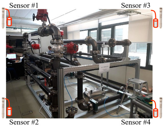
Figure 6.
Target domain data collection testbed environment using plant piping specimens.
The data collected from the source domain were preprocessed using the methods detailed in Section 2 and converted into 65,985 RMS and frequency features. To assess the performance of the proposed model in detecting leaks, the time- and frequency-domain data were divided into training and test sets using the hold-out method, with a split ratio of 6:4. The source domain included 33,000 leak data points and 32,985 background noise data points, while the target domain comprised 33,000 combined leak and noisy data points. The training procedure involved two stages. In Stage 1, two separate models were trained independently, while in Stage 2, the proposed feature fusion model was developed. For both stages, a batch size of 128 was employed, with training conducted for 30 epochs. Binary cross-entropy was used as the loss function, and the learning rate was configured to .
4.2. Analysis of Results for the Proposed Pipe Leak Detection
Figure 7 illustrates the classification results of the models with TL and without TL (non-TL) using confusion matrices, which display the correct and incorrect classifications of leak and normal states. The non-TL model was trained end-to-end in Stage 2 without leveraging Stage 1 pre-training, as shown in Figure 4. The confusion matrix on the left demonstrates the performance of the non-TL model, correctly classifying 12,940 noise instances and 13,450 leak instances, while misclassifying one noise instance and nine leak instances. In contrast, the matrix on the right shows the results of TL model, with 12,939 noise instances and 13,458 leak instances correctly classified, and only two noise instances and one leak instance incorrectly classified. These results confirm that the proposed TL model achieves superior classification accuracy for leak and normal states by leveraging pre-trained fused features compared to the non-TL model.
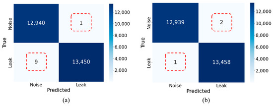
Figure 7.
Comparison of confusion matrices for model performance with and without TL: (a) results of the proposed model without TL; (b) results of the proposed model with TL.
The performance of the leak detection model was further evaluated based on precision, recall, and F1-score metrics. Precision, defined in Equation (13), quantifies the proportion of true leaks among all samples identified as leaks. Recall, defined in Equation (14), measures the proportion of actual leaks correctly detected by the model. The F1-score, shown in Equation (15), combines precision and recall into a single metric by calculating their harmonic mean.
where true positive (TP) refers to cases where the model correctly identifies a sample as a leak when it truly is one. A false positive (FP) occurs when the model incorrectly classifies a noise sample as a leak, while false negative (FN) signifies instances where the model mistakenly classifies a leak sample as noise.
Table 5 summarizes the micro-leak detection accuracies of the proposed model compared to various existing ML and DL approaches. Each model was independently trained on 1D features derived from the time and frequency domains, with their outputs combined using an ensemble approach. The multi-layer perceptron (MLP) [36,37] ensemble employed an MLP model to learn RMS and frequency features, achieving an ensemble accuracy of 80.18%. The SVM-ensemble, which employed an SVM model, achieved a higher ensemble accuracy of 85.36%. The LSTM-ensemble, combining results learned through an LSTM network, achieved an accuracy of 74.47%. The 1D CNN-based model introduced in Stage 1 learned RMS and frequency features with accuracies of 98.42% and 98.97%, respectively, culminating in an ensemble accuracy of 99.32% (1D CNN-ensemble). In contrast, the TL-based model introduced in Stage 2 of the proposed framework exhibited superior performance, achieving an exceptionally high accuracy of 99.99%.
Table 5.
Comparative analysis of accuracy in detecting low-level pipe leak.
4.3. Comprehensive Performance Analysis of the Proposed Method
Figure 8 illustrates the performance comparison among the FC-TL model, the non-TL model, and the proposed model as the dataset size decreases progressively from 100% to 1%. The FC-TL model employs transfer learning by pre-training individual models for different domains during Stage 1, as shown in Figure 4. In this stage, domain-specific features are learned independently for each domain. After training, the classifiers of the domain-specific models are removed, and feature fusion is performed to combine the extracted features from all domains. Following this step, a new classifier is added to utilize the fused features. However, the FC-TL model lacks the bidirectional LSTM and attention mechanism, which are crucial to Stage 2 of the proposed architecture, as depicted in Figure 4. While the FC-TL model effectively uses pre-trained features and benefits from transfer learning and feature fusion, its performance diminishes as the dataset size decreases. Specifically, with approximately 1% of the dataset, the FC-TL model’s accuracy drops to 83.45%. While it benefits from TL and feature fusion, the absence of mechanisms to process temporal dependencies or selectively emphasize important features limits its capability, exposing its limitations in achieving robust performance under data-scarce scenarios.
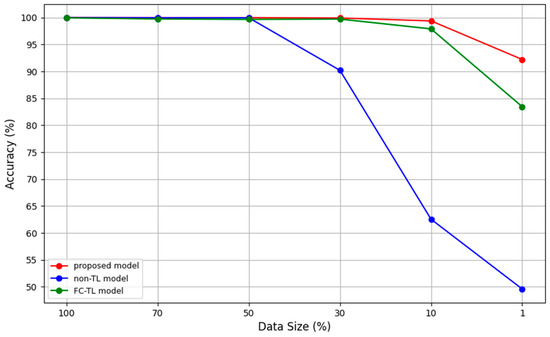
Figure 8.
Performance comparison among various models according to training data size.
The non-TL model is trained end-to-end in Stage 2 without utilizing Stage 1 pre-training, as shown in Figure 4. Unlike the FC-TL model, it does not utilize transfer learning or pre-trained features from other domains, relying solely on domain-specific features extracted during the training process. When the dataset size was large, the non-TL model performed comparably to the FC-TL model, maintaining stable accuracy. However, as the dataset size decreased, particularly below 30%, its performance declined rapidly. This significant drop demonstrates the heavy reliance of the model on a large volume of labeled data for effective learning and its limited ability to generalize in data-scarce conditions.
In contrast, the proposed model outperformed both the FC-TL and non-TL models, demonstrating exceptional robustness across all dataset sizes. Even with approximately 1% of the data, the proposed model achieved an impressive accuracy of 92.21%, far surpassing the other models. This superior performance is attributed to its efficient utilization of pre-trained features and its ability to combine diverse data through feature fusion. Furthermore, the integration of a bidirectional LSTM enables the model to process temporal information in both forward and backward directions, while the attention mechanism effectively focuses on critical features. These advanced components allow the model to differentiate leak signals from noise with high precision. These advanced components have been experimentally verified, demonstrating that the proposed model can effectively generalize and maintain consistent performance, even with minimal data.
5. Conclusions
In this study, a feature fusion leak detection model was proposed, combining TL and a bidirectional attention mechanism to identify micro-leaks in aging pipelines. The model utilized TL and feature fusion based on pre-trained information, incorporating an attention mechanism within the bidirectional LSTM to focus on critical independent features. This approach effectively addressed challenges such as data scarcity and ambient machine noise by enabling seamless transfer from the source domain to the target domain across distinct environments. A detection accuracy of 99.99% was achieved under controlled experimental conditions using a dataset comprising leak signals and ambient noise collected from multiple acoustic sensors. The ability of the model to suppress irrelevant noise and enhance key signal features through optimized signal preprocessing and feature fusion significantly contributed to this high level of accuracy. However, this exceptional performance requires further validation in real-world environments, where factors such as pipeline material variability, sensor placement, and diverse noise sources could impact the robustness of the model. Despite these potential limitations, the proposed method demonstrated strong potential for practical applications in industrial pipelines and critical infrastructure, where accurate and timely leak detection is crucial for safety and operational efficiency. Future research directions include deploying the model in embedded systems for real-time monitoring, validating its performance in diverse industrial settings, and exploring its scalability for multi-sensor environments. These efforts aim to develop a robust and adaptable early leak detection technology capable of operating effectively under real-world conditions, thereby enhancing industrial safety and efficiency.
Author Contributions
Conceptualization, Y.H. and J.-H.B.; methodology, Y.H. and J.-H.B.; software, Y.H.; validation, Y.H., Y.C., and J.L.; investigation, Y.H.; resources, Y.C.; data curation, Y.C.; draft writing and preparation, Y.H.; manuscript review and editing, J.L. and J.-H.B.; visualization, Y.H.; supervision, J.-H.B.; project administration, Y.H. and J.-H.B.; funding acquisition, Y.C. All authors have read and agreed to the published version of the manuscript.
Funding
This work was supported by the National Research Foundation of Korea through the Government (Ministry of Science and Information and Communications Technology) in 2022 under Grant RS-2022-00165225 and Grant RS-2022-00144000.
Institutional Review Board Statement
Not applicable.
Informed Consent Statement
Not applicable.
Data Availability Statement
The datasets presented in this article are not readily available because the data are part of an ongoing study and security reasons. Requests to access the datasets should be directed to the Korea Atomic Energy Research Institute.
Conflicts of Interest
The authors declare no conflicts of interest.
References
- Hussain, M.; Zhang, T.; Dwight, R.; Jamil, I. Energy pipeline degradation condition assessment using predictive analytics—Challenges, issues, and future directions. J. Pipeline Sci. Eng. 2024, 4, 100178. [Google Scholar] [CrossRef]
- Di-Sarno, L.; Majidian, A. Risk assessment of a typical petrochemical plant with ageing effects subjected to seismic sequences. Eng. Struct. 2024, 310, 118110. [Google Scholar] [CrossRef]
- Nnoka, M.; Jack, T.A.; Szpunar, J. Effects of different microstructural parameters on the corrosion and cracking resistance of pipeline steels: A review. Eng. Fail. Anal. 2024, 159, 108065. [Google Scholar] [CrossRef]
- Nati, M.; Nastasiu, D.; Stanescu, D.; Digulescu, A.; Ioana, C. Pipe leaks detection and localization using non-intrusive acoustic monitoring. In Proceedings of the 2024 15th International Conference on Communications (COMM), Bucharest, Romania, 3–4 October 2024; IEEE: Piscataway, NJ, USA, 2024; pp. 1–5. [Google Scholar] [CrossRef]
- Yan, W.; Liu, W.; Zhang, Q.; Bi, H.; Jiang, C.; Liu, H.; Wang, T.; Dong, T.; Ye, X. Multi-source multi-modal feature fusion for small leak detection in gas pipelines. IEEE Sens. J. 2023, 24, 1857–1865. [Google Scholar] [CrossRef]
- Obike, A.; Uwakwe, K.; Abraham, E.; Ikeuba, A.; Emori, W. Review of the losses and devastation caused by corrosion in the Nigeria oil industry for over 30 years. Int. J. Corros. Scale Inhib. 2020, 9, 74–91. [Google Scholar] [CrossRef]
- Wang, T.; Wang, X.; Wang, B.; Fan, W. Gas leak location method based on annular ultrasonic sensor array. In Proceedings of the 2018 IEEE International Instrumentation and Measurement Technology Conference (I2MTC), Houston, TX, USA, 14–17 May 2018; IEEE: Piscataway, NJ, USA, 2018; pp. 1–6. [Google Scholar] [CrossRef]
- Schenck, A.; Daems, W.; Steckel, J. AirleakSlam: Detection of pressurized air leaks using passive ultrasonic sensors. In Proceedings of the 2019 IEEE SENSORS, Montreal, QC, Canada, 27–30 October 2019; IEEE: Piscataway, NJ, USA, 2019; pp. 1–4. [Google Scholar] [CrossRef]
- Exaudi, K.; Passarella, R.; Rendyansyah; Zulfahmi, R. Using pressure sensors towards pipeline leakage detection. In Proceedings of the 2018 International Conference on Electrical Engineering and Computer Science (ICECOS), Las Vegas, NV, USA, 2–4 October 2018; IEEE: Piscataway, NJ, USA, 2018; pp. 89–92. [Google Scholar] [CrossRef]
- Jiao, J.; Zhang, J.; Ren, Y.; Li, G.; Wu, B.; He, C. Sparse representation of acoustic emission signals and its application in pipeline leak location. Measurement 2023, 216, 112899. [Google Scholar] [CrossRef]
- Yeo, D.; Bae, J.H.; Lee, J.C. Unsupervised learning-based pipe leak detection using deep auto-encoder. J. Korea Soc. Comput. Inf. 2019, 24, 21–27. [Google Scholar] [CrossRef]
- Jordan, M.I.; Mitchell, T.M. Machine learning: Trends, perspectives, and prospects. Science 2015, 349, 255–260. [Google Scholar] [CrossRef]
- Rane, N.; Mallick, S.; Kaya, O.; Rane, J. Techniques and optimization algorithms in machine learning: A review. In Applied Machine Learning and Deep Learning: Architectures and Techniques; CRC Press: Boca Raton, FL, USA, 2024; pp. 39–58. [Google Scholar] [CrossRef]
- Selmy, H.A.; Mohamed, H.K.; Medhat, W. Big data analytics deep learning techniques and applications: A survey. Inf. Syst. 2024, 120, 102318. [Google Scholar] [CrossRef]
- Gao, J.; Heng, F.; Yuan, Y.; Liu, Y. A novel machine learning method for multiaxial fatigue life prediction: Improved adaptive neuro-fuzzy inference system. Int. J. Fatigue 2024, 178, 108007. [Google Scholar] [CrossRef]
- Meghraoui, K.; Sebari, I.; Pilz, J.; Ait El Kadi, K.; Bensiali, S. Applied deep learning-based crop yield prediction: A systematic analysis of current developments and potential challenges. Technologies 2024, 12, 43. [Google Scholar] [CrossRef]
- Chen, J.; Chen, G.; Li, J.; Du, R.; Qi, Y.; Li, C.; Wang, N. Efficient seismic data denoising via deep learning with improved MCA-SCUNet. IEEE Trans. Geosci. Remote Sens. 2024, 62, 5903614. [Google Scholar] [CrossRef]
- Plathottam, S.J.; Rzonca, A.; Lakhnori, R.; Iloeje, C.O. A review of artificial intelligence applications in manufacturing operations. J. Adv. Manuf. Process. 2023, 5, e10159. [Google Scholar] [CrossRef]
- Waltersmann, L.; Kiemel, S.; Stuhlsatz, J.; Sauer, A.; Miehe, R. Artificial intelligence applications for increasing resource efficiency in manufacturing companies—A comprehensive review. Sustainability 2021, 13, 6689. [Google Scholar] [CrossRef]
- Arinze, C.A.; Izionworu; Onuegbu, V.; Isong, D.; Daudu, C.D.; Adefemi, A. Integrating artificial intelligence into engineering processes for improved efficiency and safety in oil and gas operations. Open Access Res. J. Eng. Technol. 2024, 6, 039–051. [Google Scholar] [CrossRef]
- Rahimi, M.; Alghassi, A.; Ahsan, M.; Haider, J. Deep learning model for industrial leakage detection using acoustic emission signal. Informatics 2020, 7, 49. [Google Scholar] [CrossRef]
- Kwon, S.; Jeon, S.; Park, T.J.; Bae, J.H. Automatic weight redistribution ensemble model based on transfer learning to use in leak detection for the power industry. Sensors 2024, 24, 4999. [Google Scholar] [CrossRef]
- Hu, X.; Zhang, H.; Ma, D.; Wang, R. A tnGAN-based leak detection method for pipeline network considering incomplete sensor data. IEEE Trans. Instrum. Meas. 2020, 70, 3510610. [Google Scholar] [CrossRef]
- Mysorewala, M.F.; Cheded, L.; Ali, I.M.; Alshebeili, S.; Alotaibi, A.B.; Al-Fakheri, F.M.; Haque, M. Leak detection using flow-induced vibrations in pressurized wall-mounted water pipelines. IEEE Access 2020, 8, 188673–188687. [Google Scholar] [CrossRef]
- Ahmad, S.; Ahmad, Z.; Kim, C.H.; Kim, J.M. A method for pipeline leak detection based on acoustic imaging and deep learning. Sensors 2022, 22, 1562. [Google Scholar] [CrossRef] [PubMed]
- Pan, S.J.; Yang, Q. A survey on transfer learning. IEEE Trans. Knowl. Data Eng. 2009, 22, 1345–1359. [Google Scholar] [CrossRef]
- Chen, X.; Yang, R.; Xue, Y.; Huang, M.; Ferrero, R.; Wang, Z. Deep transfer learning for bearing fault diagnosis: A systematic review since 2016. IEEE Trans. Instrum. Meas. 2023, 72, 3508221. [Google Scholar] [CrossRef]
- Guo, L.; Lei, Y.; Xing, S.; Yan, T.; Li, N. Deep convolutional transfer learning network: A new method for intelligent fault diagnosis of machines with unlabeled data. IEEE Trans. Ind. Electron. 2018, 66, 7316–7325. [Google Scholar] [CrossRef]
- Sak, H.; Senior, A.; Beaufays, F. Long short-term memory recurrent neural network architectures for large scale acoustic modeling. In Proceedings of the Interspeech 2014, Singapore, 14–18 September 2014; pp. 338–342. [Google Scholar] [CrossRef]
- Alawneh, L.; Mohsen, B.; Al-Zinati, M.; Shatnawi, A.; Al-Ayyoub, M. A comparison of unidirectional and bidirectional LSTM networks for human activity recognition. In Proceedings of the 2020 IEEE International Conference on Pervasive Computing and Communications Workshops (PerCom Workshops), Austin, TX, USA, 23–27 March 2020; IEEE: Piscataway, NJ, USA, 2020; pp. 1–6. [Google Scholar] [CrossRef]
- Atef, S.; Eltawil, A.B. Assessment of stacked unidirectional and bidirectional long short-term memory networks for electricity load forecasting. Electr. Power Syst. Res. 2020, 187, 106489. [Google Scholar] [CrossRef]
- Siami-Namini, S.; Tavakoli, N.; Namin, A.S. The performance of LSTM and BiLSTM in forecasting time series. In Proceedings of the 2019 IEEE International Conference on Big Data (Big Data), Los Angeles, CA, USA, 9–12 December 2019; IEEE: Piscataway, NJ, USA, 2019; pp. 3285–3292. [Google Scholar] [CrossRef]
- Luong, M.T. Effective approaches to attention-based neural machine translation. In Proceedings of the 2015 Conference on Empirical Methods in Natural Language Processing (EMNLP), Lisbon, Portugal, 17–21 September 2015; pp. 1412–1421. [Google Scholar] [CrossRef]
- Bae, J.H.; Yeo, D.Y.; Yoon, D.B.; Oh, S.W.; Kim, G.J.; Kim, N.S.; Pyo, C.S. Deep-learning-based pipe leak detection using image-based leak features. In Proceedings of the 2018 IEEE International Conference on Image Processing (ICIP), Athens, Greece, 7–10 October 2018; IEEE: Piscataway, NJ, USA, 2018; pp. 2361–2365. [Google Scholar]
- Choi, Y.R.; Lee, J.C.; Cho, J.W. A technology of micro-leak detection. In Proceedings of the Korean Society of Computer Information Conference; Korean Society of Computer Information: Seoul, Republic of Korea, 2021; pp. 685–687. [Google Scholar]
- Rumelhart, D.E.; Hinton, G.E.; Williams, R.J. Learning representations by back-propagating errors. Nature 1986, 323, 533–536. [Google Scholar] [CrossRef]
- Hornik, K.; Stinchcombe, M.; White, H. Multilayer feedforward networks are universal approximators. Neural Netw. 1989, 2, 359–366. [Google Scholar] [CrossRef]
Disclaimer/Publisher’s Note: The statements, opinions and data contained in all publications are solely those of the individual author(s) and contributor(s) and not of MDPI and/or the editor(s). MDPI and/or the editor(s) disclaim responsibility for any injury to people or property resulting from any ideas, methods, instructions or products referred to in the content. |
© 2024 by the authors. Licensee MDPI, Basel, Switzerland. This article is an open access article distributed under the terms and conditions of the Creative Commons Attribution (CC BY) license (https://creativecommons.org/licenses/by/4.0/).