1. Introduction
With the steady improvement of China’s socio-economic development and the continuous expansion of urban and industrial scales, the existing pipeline systems in China have gradually become insufficient to meet the demands of future development. The General Office of the State Council has clearly outlined in the “Implementation Plan for the Renovation and Upgrading of Aging Urban Gas Pipelines (2022–2025)” [
1] that urban gas, water supply, drainage, heating, and other aging pipelines and facilities that have outdated materials, long service lives, safety hazards in operational environments, or fail to meet relevant standards and regulations should be included as targets for renovation and upgrading. At the same time, to implement the “Energy Saving and Carbon Reduction Action Plan” [
2] proposed by the State Council, reasonable optimization and regulation of the daily use of pipeline systems can effectively reduce system power consumption, improve operational efficiency, and promote the comprehensive green transformation of economic and social development.
In the design of gas supply pipeline systems, complex hydraulic modeling calculations are often required [
3]. Due to errors in the measurement data of various component parameters of the model compared to real values, as well as potential issues such as wear and deformation at interface points during field installation, coupled with simplified measures used in some calculation processes, the final calculation accuracy often cannot meet the required standards and requires subsequent adjustments. At the same time, under the premise of meeting the user’s gas demand, rationally configuring the pressure and flow of gas supply ends can effectively reduce power consumption, save costs.
Correcting errors in pipeline system calculations and configuring gas parameters at supply ends are critical optimization problems in engineering. Swarm intelligence optimization algorithms, inspired by the collective behavior of biological populations, leverage information exchange and cooperation within groups to identify optimal solutions. Ant Colony Optimization (ACO) [
4], inspired by the foraging behavior of ants depositing pheromones to guide optimal paths, efficiently solves combinatorial optimization problems through iterative path improvement. Particle Swarm Optimization (PSO) [
5], drawing from the social behavior of bird flocks or fish schools, excels in continuous optimization problems tuning by iteratively updating particle positions for efficient convergence. Genetic Algorithm (GA) [
6], based on natural selection and genetics, uses selection, crossover, and mutation to evolve solutions, making it effective for complex, multi-dimensional problems. Simulated Annealing (SA) [
7], inspired by the metallurgical annealing process, explores solution spaces by accepting worse solutions with decreasing probability to escape local optima. Coyote Optimization Algorithm (COA) [
8] mimics the social and hunting behaviors of coyotes, balancing exploration and exploitation for high-dimensional problems. Teaching–Learning-Based Optimization (TLBO) [
9], inspired by classroom learning, uses teacher and learner phases to iteratively improve solutions, offering simplicity and effectiveness. Gray Wolf Optimizer (GWO) [
10], inspired by the leadership hierarchy and hunting strategies of gray wolves, is highly effective for high-dimensional and multimodal problems, ensuring stable and accurate convergence through balanced exploration and exploitation. Zebra Optimization Algorithm (ZOA) [
11], inspired by zebras’ social and survival behaviors, efficiently navigates complex solution spaces, offering robust performance for dynamic systems. By integrating the unique attributes of these biological populations, these algorithms significantly enhance solution accuracy and stability, opening broader and more efficient avenues for optimization research and applications.
Recent advancements in intelligent optimization algorithms have significantly enhanced the performance of gas pipeline systems by addressing challenges in error correction, fault diagnosis, and network design. For instance, Wei et al. [
12] developed a stochastic optimization algorithm integrating PSO with high-fidelity simulation to optimize large-scale natural gas pipeline networks, reducing energy consumption by up to 21.23% and correcting simulation errors in pressure and flow for a network with 43 pipeline sections and four compressor stations. Similarly, Ramos et al. [
13] proposed a multi-criteria optimization approach using metaheuristic algorithms, such as simulated annealing and ACO, to design natural gas pipeline network expansions under load-evolution uncertainty, achieving robust performance through Monte-Carlo simulation and dominance analysis, outperforming conventional design methods. Furthermore, Yao et al. [
14] introduced a cross-domain generative diagnosis method combining deep learning and genetic algorithms to enhance oil and gas pipeline defect diagnosis under limited field data, improving diagnostic accuracy by 7.21–12.79% through optimized feature distribution and noise constraint strategies. These studies demonstrate the transformative potential of intelligent optimization algorithms in improving the accuracy, efficiency, and reliability of gas pipeline systems.
This paper employs a Gray Wolf Optimizer (GWO)-based method to reduce calculation errors and a Zebra Optimization Algorithm (ZOA)-based approach for optimizing gas supply pressure distribution.
Section 2 introduces the conventional solution process for looped pipeline network systems.
Section 3 describes the principles of the GWO and ZOAs.
Section 4 presents the experimental design, results, and analysis.
Section 5 provides a summary and future outlook.
2. Materials and Methods
2.1. Solution Process
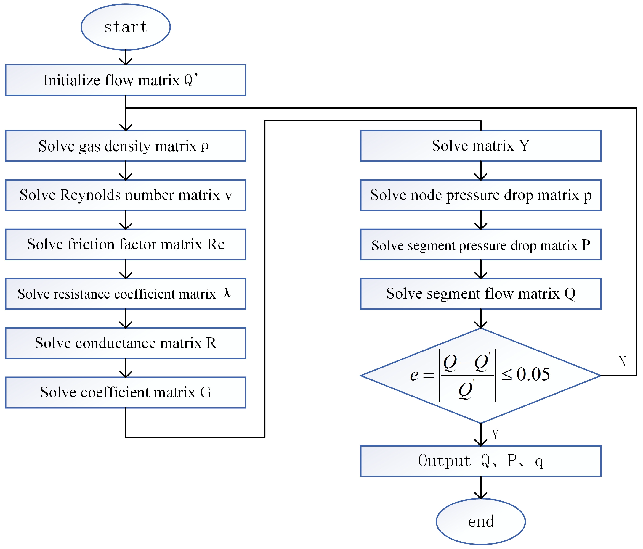
In the static model of compressed gas transportation and distribution systems, solving ring-type pipeline networks is typically performed using the node equation method. The node equation method is based on the continuity equations at the nodes. It starts by setting initial flow values for the pipeline segments, calculating the resistance coefficients for each pipeline, and then determining the system’s node pressure drops, flow rates, and other parameters based on the node flow and pipeline network topology. The flow is then adjusted, and after several iterations, the unknown variables are solved. This method is highly flexible, suitable for handling complex networks with multiple gas sources, and well-suited for computer-based solutions [
15,
16,
17]. The process is shown in
Figure 1.
The computation commences with an initial assumption of the flow rate, , for each pipe segment. This initial value is then utilized to calculate a series of hydraulic parameters, including the gas density , Reynolds number , Darcy-Weisbach friction factor , and the pipe resistance coefficient . Subsequently, the algorithm enters a core iterative loop, where a system of network equations describing the flow balance at each node is first established and solved to obtain the nodal pressures, . Based on these pressures, the pressure drop across each segment is calculated, which is in turn used to update the segment flow rate Q. Convergence is then assessed by comparing the relative change between the flow rates from the current and previous iterations. If the maximum relative change falls below a predefined tolerance (e.g., 5%), the iteration terminates, and the final results for flow rates (), pressure drops (), and nodal pressures () are outputted. Otherwise, the newly computed flow rates are used as the input for the subsequent iteration, and the loop repeats until the convergence criterion is satisfied.
2.2. Connectivity Matrix
The actual pipeline network system can be simplified as a directed linear graph composed of several nodes and pipelines. The full connectivity matrix of the graph is an matrix, where represents the number of nodes, and represents the number of pipeline segments. The rows correspond to node indices , and the columns correspond to branch indices . The values in the matrix are arranged as −1, 1, or 0:0 indicates that node is not on branch , 1 indicates that node is at the end of branch , and −1 indicates that node is at the start of branch In the node equations, any equation can be obtained by summing the other equations. Therefore, only an matrix is needed to describe the connectivity of a pipeline network. This matrix is referred to as the connectivity matrix of the network.
2.3. Matrix Representation of the Basic Equations
The mathematical expression of the current pipeline network calculation formula can generally be summarized as , where represents the pressure drop across the pipeline segment, is the pipeline segment’s resistance, and is the flow rate through the pipeline segment. Since , the relationship between pressure drop and flow rate is nonlinear. If we rewrite as , and let be represented as , we get , which transforms the original nonlinear relationship between pressure drop and flow rate into a linear one.
The pipeline segment flow rate and node flow rate satisfy Equation (1), while the pipeline segment pressure drop and node pressure drop satisfy Equation (2). Moreover, based on the formulas
and
, Equation (3) can be derived.
For the convenience of calculation, the above equation is simplified by letting
, which results in Equation (4). Here, the matrix
is the conductance matrix,
is the coefficient matrix.
2.4. Multi-Gas Source Node Solution
In this case, the number of the reference gas source node is arranged after the other nodes (with the pressure reference point having the highest number). If there are
known pressure gas sources, aside from the “reference point,” since the node flow rates are all unknown and the pressure drops relative to the “reference point” are known, it is only necessary to solve
equations when solving the node equation system (where
is the total number of nodes). The coefficient matrix is divided into four blocks:
(where
rows and
rows,
columns and
columns. The column vectors
and
are also divided into two parts. The system of equations is as follows:
According to the matrix block multiplication rule, matrix Equation (6) can be obtained. It can be seen that by appropriately modifying the node flow rates of the nodes adjacent to nodes
to
, the node linear equation system can be solved.
2.5. Pipeline Resistance Coefficient Calculation
In a compressed air system, common components include straight pipes, elbows, reducers, tee joints, valves, etc. Since the calculation of the resistance coefficient for tee joints is relatively complex, it is omitted in this process. To calculate the pipeline segment resistance coefficient
, it is necessary to first sequentially determine the gas density
, flow velocity
, Reynolds number
, and friction loss coefficient
along the pipe. The formulas for density, flow velocity, Reynolds number, and friction loss coefficient are as follows:
The meanings and units of the various symbols are shown in
Table 1. Among them, the friction coefficient can be obtained from tables. In practical use, due to installation errors and material aging, the friction coefficient values often need to be appropriately adjusted to meet actual requirements.
The resistance coefficient for straight pipeline segments is calculated using Equation (11). For elbows, Equation (12) is used, where the elbow angle
is 90° and
. When
is not 90°,
is determined by Equation (13). The resistance coefficient for reducers is calculated using Equation (14). When the mainstream direction changes from smaller to larger,
is obtained using Equation (15); when the mainstream direction changes from larger to smaller,
is obtained using Equation (16).
and
represent the cross-sectional areas of the outlet and inlet,
is the half apex angle of the variable diameter. The resistance coefficient for valves is calculated using Equation (17). For gate valves,
; for globe valves,
; the value for ball valves can be found in the table.
4. Experiment and Analysis
4.1. Introduction to the Experimental Model
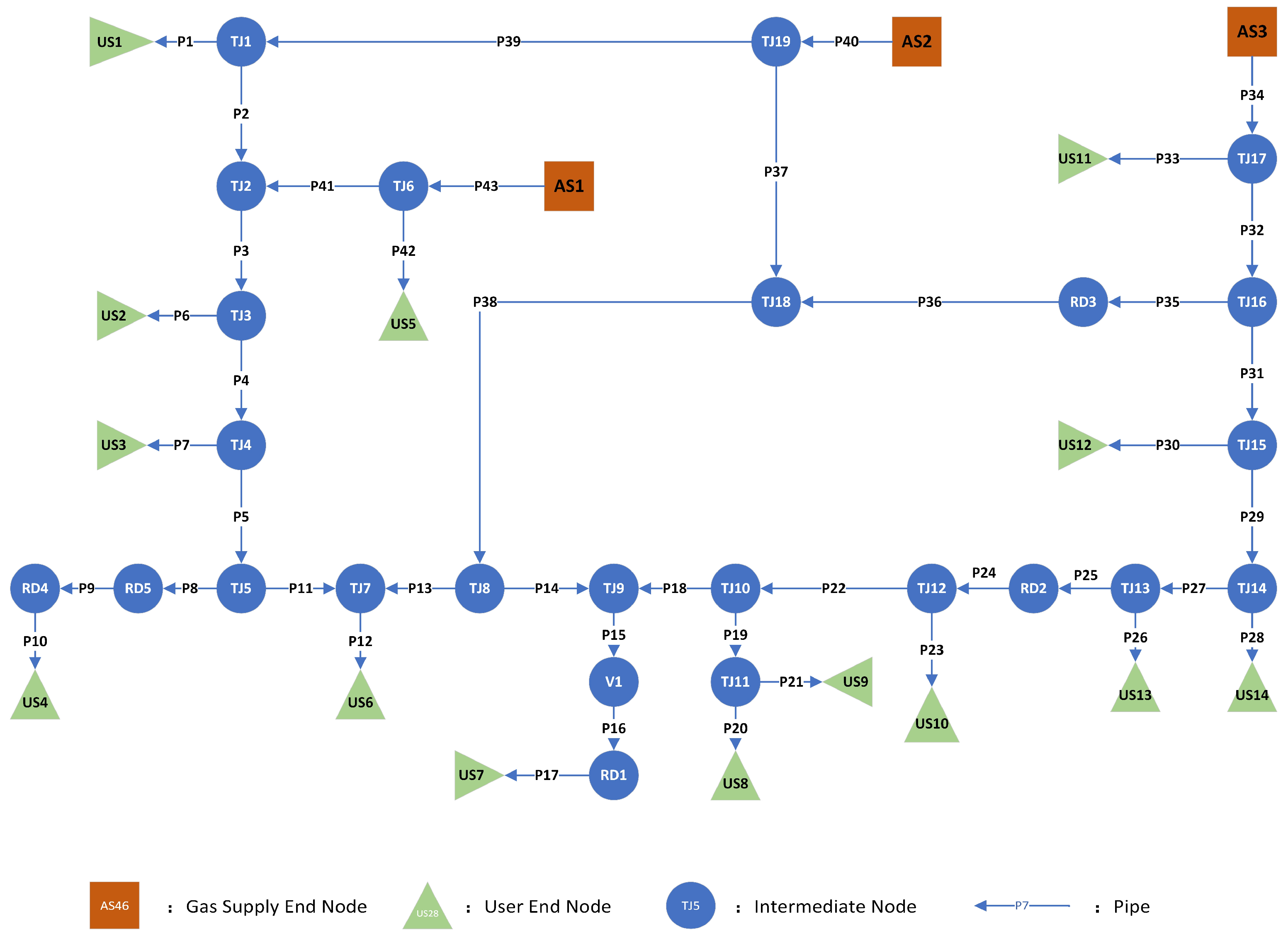
This study utilizes a network model illustrated in
Figure 2, which is established based on an actual compressed air transmission and distribution system from an industrial park in Northern China. The model consists of 3 supply nodes, 14 user end nodes, and 43 composite pipelines. Detailed parameters for the system are provided in
Appendix A.
The gas transported within the pipelines is assumed to be compressed air at 20 °C with a dynamic viscosity of
. Given a set of pressure values for the supply nodes (AS1, AS2, AS3), the iteration process is carried out based on the method described in
Section 2. After each iteration, the pipeline flow rates are compared with the results from the previous iteration. The iteration is stopped when the largest change in the flow rate of any pipeline is less than 0.5%. To prevent numerical divergence toward zero during the iteration, a maximum iteration limit of 30 rounds is set. After the iteration is completed, the calculation results are checked. If the pressure at any user-end node or the flow rate in any pipeline exceeds the design limits, the pressure combination of the supply nodes for that case is considered an invalid solution.
All development and performance evaluations were conducted on a workstation with the following specifications. The software stack comprised Microsoft Windows 11 Pro (64-bit), the .NET 8.0 framework, and Microsoft Visual Studio Community 2022 (Version 17.14.9) as the IDE. The hardware platform was equipped with an Intel Core i5-13600KF processor and 32 GB of RAM (Intel, Santa Clara, CA, USA).
4.2. Evaluation Metrics and Parameter Settings
In the pipeline network system error correction experiment, the Error between the calculated pipeline flow values and the true values is used as the evaluation metric for the algorithm. The calculation formula is as follows:
In Equation (32),
represents the number of pipelines, and
and
represent the true flow and the calculated flow of the
-th pipeline, respectively. In the gas supply end pressure distribution experiment, three indicators—gas supply end pressure, system power, and energy efficiency—are considered comprehensively. The formula is as follows:
In Equations (32)–(35), represents the system power, is the number of gas supply end nodes, and and represent the pressure and flow at the -th node, respectively. , and are constants related to the performance of the compressor equipment at the gas supply end, and they are known in this experiment. represents the system energy efficiency, and is the number of user end nodes. denotes atmospheric pressure. is a comprehensive evaluation metric, where represents the minimum achievable pressure at the gas supply end. This metric aims to minimize both the system power and the gas supply end pressure, while maximizing the system’s energy efficiency.
To validate the superiority of the algorithm used in this experiment, several classic optimization algorithms were selected for the comparison experiment. The main parameter settings for each algorithm are shown in
Table 2. In this study, to eliminate the confounding effects of initial randomness on algorithm performance evaluation and to ensure a fair comparison among different optimization algorithms, we rigorously controlled for stochasticity in our experimental process. Specifically, before the commencement of each independent run, a global random seed was set to generate the initial solution set for the algorithm. This procedure ensures that all evaluated optimizers start from the identical set of initial solutions, and consequently, the final performance differences can be directly attributed to the intrinsic characteristics of the algorithms themselves.
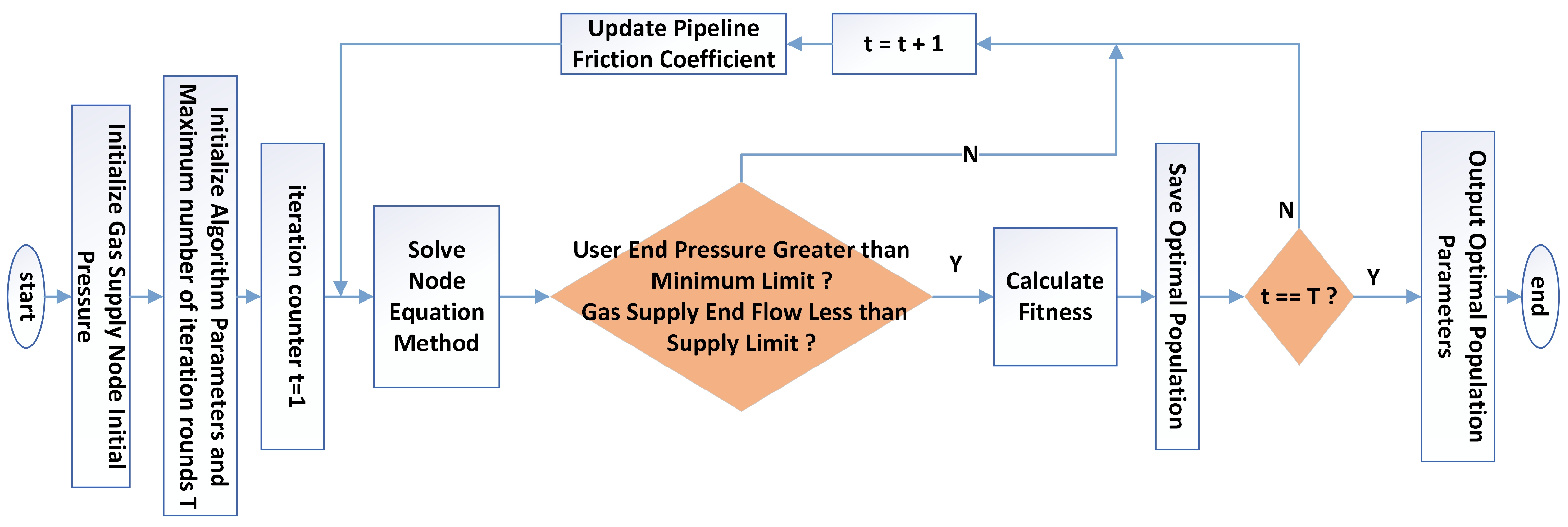
4.3. Error Correction Based on GWO
In the operation of gas supply pipeline networks, there is often a deviation between on-site measured parameters and model calculation results. The causes of this deviation are complex, and it is difficult to fully identify and precisely correct the related parameters manually, which may affect operational efficiency and safety. Therefore, there is an urgent need to introduce intelligent optimization algorithms to dynamically adjust and optimize system parameters. Since the pipeline length and diameter are fixed values, the friction coefficient
of each pipeline is chosen as the random variable to be adjusted, with a value range of [0.1, 0.5]. Since the node pressure values are relatively high and the calculation results show small deviations, the absolute sum of the differences between the real flow values and the measured values of seven random pipelines in the system (as shown in
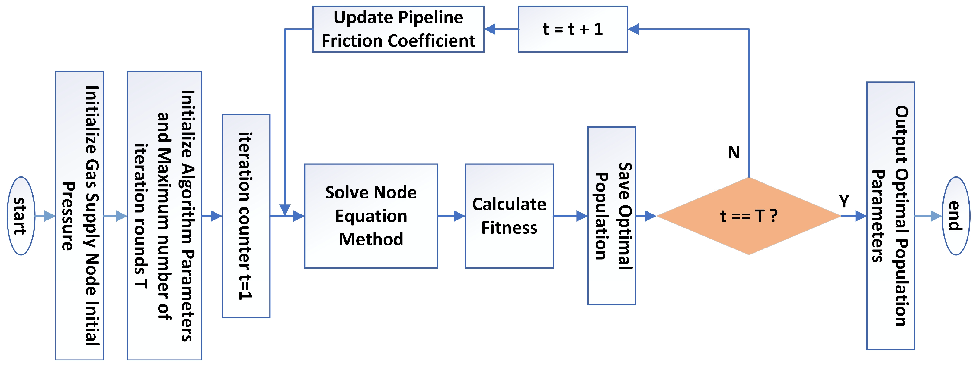
Figure 2), namely P1, P2, P3, P41, P43, P45, and P53, is used as the fitness value. This value is then substituted into the fitness function to drive the model to approach actual operating conditions. The specific process is shown in
Figure 3.
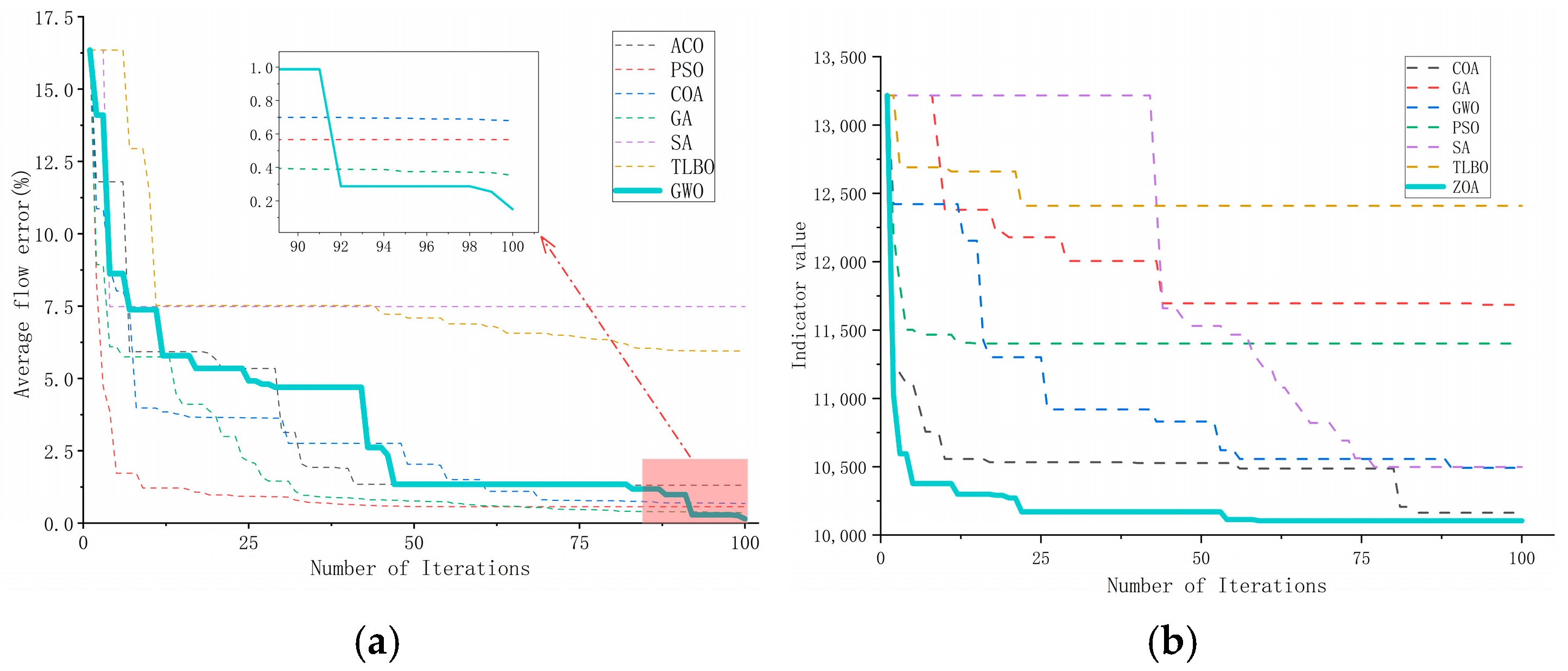
The experimental results (see
Table 3 and the fitness curve in
Figure 4a) show that most swarm intelligence algorithms can effectively reduce model errors, but there are significant performance differences. It is noteworthy that although Particle Swarm Optimization (PSO) and Genetic Algorithm (GA) exhibited fast convergence in the early stages, with a rapid decrease in fitness values, they soon entered a stagnation phase, and their final accuracies (0.56% and 0.35%, respectively) were not optimal. This strongly suggests that they may have fallen into local optima, which is attributed to the complex coupling relationships that may exist between multiple friction coefficient variables in the error correction problem and the resulting rugged fitness landscape.
Specifically, PSO simulates the social behavior of particles, each exploring the solution space to find the optimal solution. While PSO converges rapidly towards the global optimum, it is prone to premature convergence, especially in complex, multi-modal optimization problems such as error correction in supply networks. The balance between exploration and exploitation is primarily determined by the position of the best particle, which may restrict the exploration of alternative solution regions, thereby increasing the risk of stagnation. Additionally, PSO lacks a diversity-preserving mechanism, which often leads to a loss of search diversity in the later stages of optimization.
Similarly, GA employs genetic operators (selection, crossover, and mutation) to evolve the population towards an optimal solution. Although GA is theoretically capable of exploring a large search space, its convergence can be slow and susceptible to local optima, particularly in high-dimensional problems. The randomness introduced by mutation and crossover is beneficial for global search in the early stages; however, as the population converges, the algorithm may struggle to generate meaningful new candidates, leading to stagnation.
In contrast, the Gray Wolf Optimizer performed excellently in this task, achieving the lowest average relative error (0.15%) among all algorithms, while its computational efficiency (6.16 s) is comparable to faster algorithms such as PSO (5.89 s) and ACO (4.15 s), demonstrating a good balance between accuracy and efficiency. The superiority of GWO can be attributed to its unique biomimetic mechanism: first, it simulates the social hierarchy of wolf packs, where the Alpha, Beta, and Delta leaders collectively guide the population search. This provides richer and more diverse exploration directions compared to single global optimal guidance (such as PSO) or probabilistic selection (such as GA), which helps in conducting a comprehensive search in a multidimensional solution space; second, it uses a control parameter that linearly decreases from 2 to 0, achieving an adaptive and smooth transition from global exploration to local exploitation, ensuring a broad search in the early stages.
Therefore, GWO has significant advantages in handling error correction problems with potential local optimum traps, due to its intrinsic mechanism. Even if the Alpha wolf temporarily falls into a local optimum, the presence of the Beta and Delta wolves provides alternative directions, guiding the population to continue exploring. This effectively explains why the GWO curve in
Figure 4a steadily declines in the middle and later stages and ultimately outperforms other algorithms. In conclusion, GWO, with its hierarchical guiding strategy and dynamic balance between exploration and exploitation, efficiently addresses the challenges of multi-variable, highly coupled, and local optimum-prone parameter correction in supply network models.
4.4. Pressure Distribution Based on ZOA
In this experiment, the fitness value and algorithm evaluation metric are both denoted as
, with the pressure values of the three gas supply end nodes in
Figure 2 used as the adjustable random variables. The experimental process is shown in
Figure 5. In engineering practice, different combinations of gas supply end pressures correspond to different flow combinations. The calculated flow must be less than the maximum output limit of the gas supply nodes, while the pressure at the user end usually has a lower limit (set to 700 kPa in this experiment). Therefore, when applying the optimization algorithm, it is necessary to check whether the output results meet the above constraints. If the results do not meet the constraints, recalculation is required until a feasible solution is obtained. Compared to the error correction problem, this problem places higher demands on the global search ability and computational efficiency of the algorithm.
The experimental results of gas supply end pressure distribution are shown in
Figure 4b and
Table 4. In this problem, the performance differentiation of the algorithms is more pronounced. The Zebra Optimization Algorithm (ZOA) stands out, with its fitness curve (
Figure 5) not only starting with a lower initial value but also declining the most rapidly, ultimately achieving the best evaluation value (10,105.47) among all the algorithms. This indicates that ZOA possesses strong global search capability and efficient convergence characteristics for this problem.
ZOA’s success likely stems from its unique integration of foraging and defense strategies. The foraging phase (moving toward the optimal solution) ensures rapid convergence to high-quality areas, explaining the steep fitness curve decline in
Figure 5. Crucially, its defense strategy—particularly the random rapid movement simulating predator evasion—provides powerful local optimum escape capability. The pressure distribution problem optimizes a comprehensive Indicator (including system power consumption, energy efficiency, and pressure levels) under constraints like minimum user pressure and station flow limits, creating a complex, constrained optimization space. ZOA’s defense mechanism helps populations escape constraint boundaries or local optima for renewed exploration. Its good point set initialization may also offer a more favorable starting point.
In contrast, while GA (4.20 s), PSO (6.24 s), and GWO (6.25 s) ran faster, their higher final evaluation values indicate insufficient robustness. This suggests their search mechanisms are less effective than ZOA’s at handling the problem’s complex constraints or multi-objective optimization (energy consumption, efficiency, pressure). They more readily converge to constraint-satisfying but suboptimal solutions, lacking ZOA’s explicit deadlock-breaking defense strategy. Although Coyote Optimization Algorithm (COA) showed strong global search capability, its results still trailed ZOA. Thus, for gas supply pressure distribution with complex constraints and multiple objectives, ZOA demonstrates superior applicability.
5. Conclusions and Outlook
This paper addresses the error correction and gas supply-end pressure distribution problems in gas supply pipeline systems, applying the Gray Wolf Optimization Algorithm and Zebra Optimization Algorithm to solve these problems, and comparing them with other optimization algorithms. The research results show that, in the error correction problem, GWO demonstrates excellent performance with an average relative error of only 0.15%, achieving the highest accuracy among all the compared algorithms, and significantly high computational efficiency (only 6.16 s for 100 iterations). In the gas supply-end pressure distribution problem, ZOA exhibits the fastest convergence speed and the highest fitness value, ultimately achieving the optimal evaluation value of 10,105.47, significantly outperforming other algorithms.
There are still many areas worth exploring for optimizing gas supply pipeline systems: in algorithm integration and improvement, multiple optimization algorithms can be combined to further enhance the global search ability and computational efficiency; in dynamic optimization and real-time regulation, dynamic optimization algorithms combined with real-time data monitoring can be explored to realize real-time regulation and operation of pipeline systems. In the future, further efforts are needed to address the engineering challenges of these algorithms, improve their stability, scalability, and user-friendliness, and provide strong support for the efficient operation and sustainable development of pipeline systems.
Looking forward, further research can focus on integrating these algorithms into hybrid approaches, combining the strengths of multiple optimization techniques to enhance global search capabilities and computational efficiency. Additionally, real-time optimization and dynamic regulation could be achieved by integrating these algorithms with SCADA (Supervisory Control and Data Acquisition) systems, enabling live monitoring and adjustment of pipeline parameters. This integration could lead to significant improvements in operational efficiency, safety, and sustainability, providing valuable support for the future of smart energy systems.
