Article

Real-Time Global Velocity Profile Calculation for Eco-Driving on Long-Distance Highways Using Variable-Step Spatial Segmentation

1
Graduate School of Automobile and Mobility, Kookmin University, Seoul 02707, Republic of Korea
2
Department of Cogno-Mechatronics Engineering, Pusan National University, Busan 46241, Republic of Korea
3
Department of Automobile and IT Convergence, Kookmin University, Seoul 02707, Republic of Korea
*
Author to whom correspondence should be addressed.
Appl. Sci. 2025, 15(19), 10811; https://doi.org/10.3390/app151910811
Submission received: 5 September 2025 / Revised: 30 September 2025 / Accepted: 7 October 2025 / Published: 8 October 2025

Abstract

This study introduces a real-time optimization framework for eco-driving of heavy-duty vehicles over long-distance routes. A longitudinal dynamic model incorporating powertrain performance and fuel consumption is formulated, and the eco-driving scenario is expressed as a quadratic programming (QP) problem. To improve computational efficiency, a novel variable-step spatial segmentation method is introduced, which ensures a balance between modeling accuracy and computational cost. Simulations involving mixed-terrain scenarios verify the effectiveness of the proposed approach. The results show that the QP-based method achieves fuel savings comparable to those offered by dynamic programming while significantly reducing computation time to sub-second levels; thus, the proposed strategy offers real-time applicability. These findings demonstrate the feasibility of global optimal velocity profile generation in practical eco-driving scenarios.

1. Introduction

The road transportation sector is the largest contributor to greenhouse gas emissions from the transport industry, with medium-duty and heavy-duty commercial vehicles, such as trucks and buses, accounting for more than 35% of the direct C O 2 emissions from road freight. Since the pandemic, freight demand has rapidly recovered and continues to increase, which necessitates the urgent reduction in fuel consumption and emissions from commercial vehicles at both national and industrial levels [1,2].
From a logistics perspective, fuel expenses constitute a significant share of total operating costs. Improving fuel efficiency over a given distance directly yields both cost savings and carbon reduction. Driving strategies that leverage preview information (e.g., road grades and speed limits), such as predictive powertrain control or cruise control, have been repeatedly reported to deliver fuel savings of approximately 3–5% [3,4,5].
In freight operations, punctuality and travel time reliability are directly linked to service quality. The U.S. Federal Highway Administration (FHWA) introduced the Level of Travel Time Reliability (LOTTR), defined as the ratio of the 80th and 50th travel time percentiles, as a key indicator for policy and performance evaluation. This implies that optimal truck-driving strategies must simultaneously reduce fuel costs and ensure timely arrival [6,7,8].
Additionally, freight safety (preventing cargo damage, rollover, or detachment) is strictly mandated by laws and safety standards (e.g., North American cargo securement regulations). Excessive acceleration, deceleration, or oscillations should be suppressed because speed guidance and traction control are directly associated with cargo safety. Therefore, ride-comfort and acceleration constraints must be incorporated when optimizing velocity profiles [9,10].
In summary, to simultaneously satisfy requirements for (i) fuel cost and emission reduction, (ii) travel time reliability, and (iii) freight safety, optimal velocity profiles that utilize preview information, such as road slope and speed limits, must be generated while also allowing for real-time re-optimization in response to unexpected events (e.g., traffic changes or rerouting). In the context of global velocity planning, “real-time applicability” has conventionally been associated with computational frameworks operating at a minimum frequency of 1 Hz [11,12,13]. Although the necessity and sufficiency of the 1 Hz frequency may vary depending on the problem setting, defining 1 Hz as the threshold for real-time applicability is reasonable in continuous highway environments, such as the one considered in this study [14]. Consequently, the optimal eco-driving strategy for freight vehicles can be characterized as a complex multi-objective optimization problem that must balance fuel economy, travel time reliability, and cargo safety.
Eco-driving strategies can generally be categorized into two types: time-domain and space-domain formulations. The time-domain approach involves expressing the problem as a function of velocity and acceleration over time, whereas in the space-domain approach, vehicle dynamics are modeled with respect to position. The latter naturally incorporates road characteristics such as gradient, speed limits, and curvature [15]. Therefore, to directly capture the influence of road topology and physical properties on driving strategies and to maximize fuel efficiency, the space-domain approach is considered essential.
In early studies, dynamic programming (DP) was predominantly used to solve highly nonlinear optimization problems [16]. For highway truck driving, Hellström et al. [17] proposed a GPS-based look-ahead DP controller that utilizes road slope information and experimentally validated its fuel-saving potential. In a subsequent study, Hellström et al. [18] derived optimal velocity profiles for fuel efficiency using DP with linearized slope segments, confirming the energy-saving potential of this technique for heavy-duty vehicle operations. Pulvirenti et al. [19] and Zhang [13] introduced computationally efficient DP methods with variable grid discretization to derive optimal fuel-efficient speed profiles, achieving significantly faster computation compared with conventional DP. Shiedar et al. [20] proposed a hybrid framework for fuel-cell trucks, combining approximate DP-based global velocity optimization with a receding-horizon optimal control problem (OCP) to enable real-time application. Spano et al. [21] validated the performance of approximate DP-based eco-driving strategies on real-world logistics routes, observing fuel-saving benefits under realistic driving conditions.
Despite its advantages, however, a major limitation of DP is that the computation time increases rapidly with road length, which significantly hinders real-time applications. While DP guarantees global optimality, it inherently suffers from the curse of dimensionality, whereby its computational complexity increases exponentially with the size of the discretized state space.
To address the computational burden of DP and handle long-horizon optimization problems, several optimal control theory-based and numerical optimization methods have been introduced. Hamednia et al. [22] formulated a predictive velocity control problem for long look-ahead horizons on hilly terrain and discussed the potential for fuel economy improvement when considering horizons exceeding 100 km. Subsequently, Hamednia et al. [23] extended this approach by focusing on computational efficiency, devising numerical and structural methods that render global optimization more tractable and achieve near-real-time feasibility for long horizons.
Regarding electric and autonomous commercial vehicles, Zhang et al. [24] proposed an eco-driving control framework that explicitly considers highway topography. They integrated velocity profile optimization with power management (energy consumption and battery degradation) to design a control strategy that adapts to road slopes while improving both the energy efficiency and long-term battery performance of electric trucks. Finally, Li et al. [25] introduced a real-time predictive cruise control strategy for commercial vehicles based on quadratic programming (QP). By leveraging the computational efficiency of QP, they demonstrated how predictive cruise control can be implemented in real time while incorporating both road gradients and vehicle dynamics constraints.
Most of the aforementioned studies adopted a fixed-step spatial segmentation approach, which divides the road into uniform segments. While this method simplifies mathematical modeling, it also exhibits several critical limitations:
  • Loss of road topology information: If the segment length is excessively large, important geographical features, such as steep gradients within short intervals, may be overlooked. For instance, when using a 500 m step size, a steep slope within a 200 m section may be averaged with flat regions, which would lead to inaccurate representation of the actual slope. Such inaccuracies can result in critical errors when deriving fuel-optimal velocity profiles.
  • Computational inefficiency: Conversely, if a very short step size is chosen to capture fine variations in road geometry, the number of segments grows exponentially over the entire route. This dramatically increases the computational burden of optimization algorithms such as DP or nonlinear programming (NLP), thereby hindering real-time applicability. Such inefficiencies become even more pronounced on long-haul freight routes.
  • Difficulty in real-time re-optimization: In practice, unexpected events, such as changes in traffic conditions or route adjustments, necessitate rapid re-computation of the optimal velocity profile. However, under a fixed-step framework, such events increase the problem size substantially, whereby the recalculation times become too long to satisfy real-time requirements.
Recent research has extended eco-driving control to incorporate travel time reliability and cargo safety in addition to fuel efficiency, addressing the problem as a multi-objective optimization task. In freight transport, punctuality is directly linked to service quality, with the U.S. FHWA emphasizing the importance of timely arrival by introducing the LOTTR as a performance indicator. Accordingly, travel time constraints have been included in several optimization models to simultaneously achieve fuel savings and punctuality [17,22,23,26].
Moreover, as excessive acceleration or deceleration of trucks increases the risk of cargo damage, rollover, or displacement, cargo safety represents another critical consideration. Hence, acceleration and jerk terms have been incorporated into either the objective function or the constraints when planning optimal velocity profiles. Recent studies have introduced methods that minimize acceleration variations to ensure smoother driving [27,28]. However, such constraints increase the complexity of the optimization problem further, thereby limiting the feasibility of real-time computation.
To date, fuel economy, punctuality, and cargo safety have often been treated as separate problems; otherwise, when attempting multi-objective formulations, the reliance on fixed-step segmentation has resulted in significant computational challenges. To overcome these limitations, this study introduces a variable-step spatial segmentation method. This approach preserves essential road features while drastically reducing the number of segments, thereby enabling real-time computation even for long-haul routes. Furthermore, by approximating the complex nonlinear vehicle dynamics into a QP problem, the proposed framework efficiently derives globally optimal solutions. This strategy is designed to significantly advance real-time global velocity profile calculation by simultaneously satisfying the three key objectives, namely fuel efficiency, travel time reliability, and cargo safety.
The remainder of this paper is organized as follows: Section 2 presents the longitudinal dynamic model of the target vehicle, including the powertrain, driving performance, and fuel consumption formulations. Section 3 introduces the optimization framework for eco-driving, defining the optimal control problem and discussing the proposed variable-step spatial segmentation method along with the QP formulation. Section 4 presents the simulation results and related interpretations. Finally, Section 5 concludes the paper with a summary of the findings.

2. Longitudinal Dynamic Model

A longitudinal dynamic model was established for a conventional vehicle equipped with an internal combustion engine and a 12-speed transmission. The longitudinal motion of the vehicle is governed by the tractive force generated by the powertrain system and the braking force produced by the braking system. Traditionally, these two forces are designed to be mutually exclusive; thus, the corresponding longitudinal dynamics are articulated through the respective force transmission mechanisms.

2.1. Longitudinal Vehicle Dynamics

The longitudinal dynamics are formulated using a lumped-mass model, in which the travel distance (s) and vehicle speed (v) are defined as the state variables:
s ˙ t = v t , m v ˙ t = F w t + F b r k t F a e r o v F s l o p e s F r o l l ( s ) .
Here, m represents the total mass of the vehicle, including the cargo weight; F w and F b r k are the control inputs, denoting the traction force (positive) and braking force (negative), respectively; and F a e r o , F s l o p e , and F r o l l denote the driving resistances, namely the aerodynamic drag, grade resistance, and rolling resistance, respectively. In Equation (1), each component of the driving resistance is a function of time t as it varies with the travel distance and vehicle speed. However, for notational simplicity, the explicit time dependence of these components is omitted.
F a e r o v = ρ a C d A f v 2 t 2 , F s l o p e = m g sin α s , F r o l l = m g   C r   C o s α s .
In Equation (2), ρ a denotes the air density, C d represents the aerodynamic drag coefficient, A f is the frontal area of the vehicle, g denotes the gravitational acceleration, C r represents the rolling resistance coefficient, and α represents the road slope angle, which is a function of s.

2.2. Re-Parameterization of Independent Variables

In optimal speed planning for commercial vehicles traveling along a global route, representing the system states with respect to travel distance ( s ) rather than time ( t ) is more advantageous. This is because, for a fixed travel route, the key constraints and disturbances—such as road grade, surface condition, speed limits, and stopping sections—are functions of s . Consequently, modeling the states and constraints as direct functions of s ensures a more intuitive and concise representation of the route-based cost functions and constraints.
As seen in Equation (1), s increases monotonically with respect to t; therefore, the inverse function t ( s ) exists. Furthermore, the vehicle’s velocity can be expressed as a function of its position. Based on the differentiation property of inverse functions, Equation (1) can thus be rewritten as
t s = d t d s = 1 v ( t ) = 1 v ~ ( s ) .
Additionally, the quadratic term of velocity, which exhibits nonlinearity, can be expressed in terms of kinetic energy:
E s = m v 2 s 2 .
Equation (1) can be re-parameterized from the time domain t to the position domain s as follows:
t s = m 2 E ( s ) , E s = F w s + F b r k s c ~ a E s F α ( s ) ,
where c ~ a = ρ a C d A f / m and F α s = F s l o p e θ + F r o l l ( θ ) . This transformation converts all nonlinear terms in Equation (1) into linear forms.

2.3. Engine Model

The vehicle used in this study is equipped with a diesel engine producing a maximum power of 525 ps. The detailed output curves can be found in the engine characteristic map shown in Figure 1.

2.4. Transmission System

The engine power is transmitted through the gearbox and converted into longitudinal force and velocity. The power transmission process is defined by the following equation:
F w s = η t i f i g γ g r w T e , v s = π   30 r w i f i g ( γ g ) ω e ,
where η t denotes the efficiency of the transmission and drivetrain, i f is the final reduction ratio, i g ( γ g ) represents the gear ratio as a function of the transmission gear ( γ g ) , and r w is the wheel radius.

2.5. Driving Performance and Maximum Force Approximation

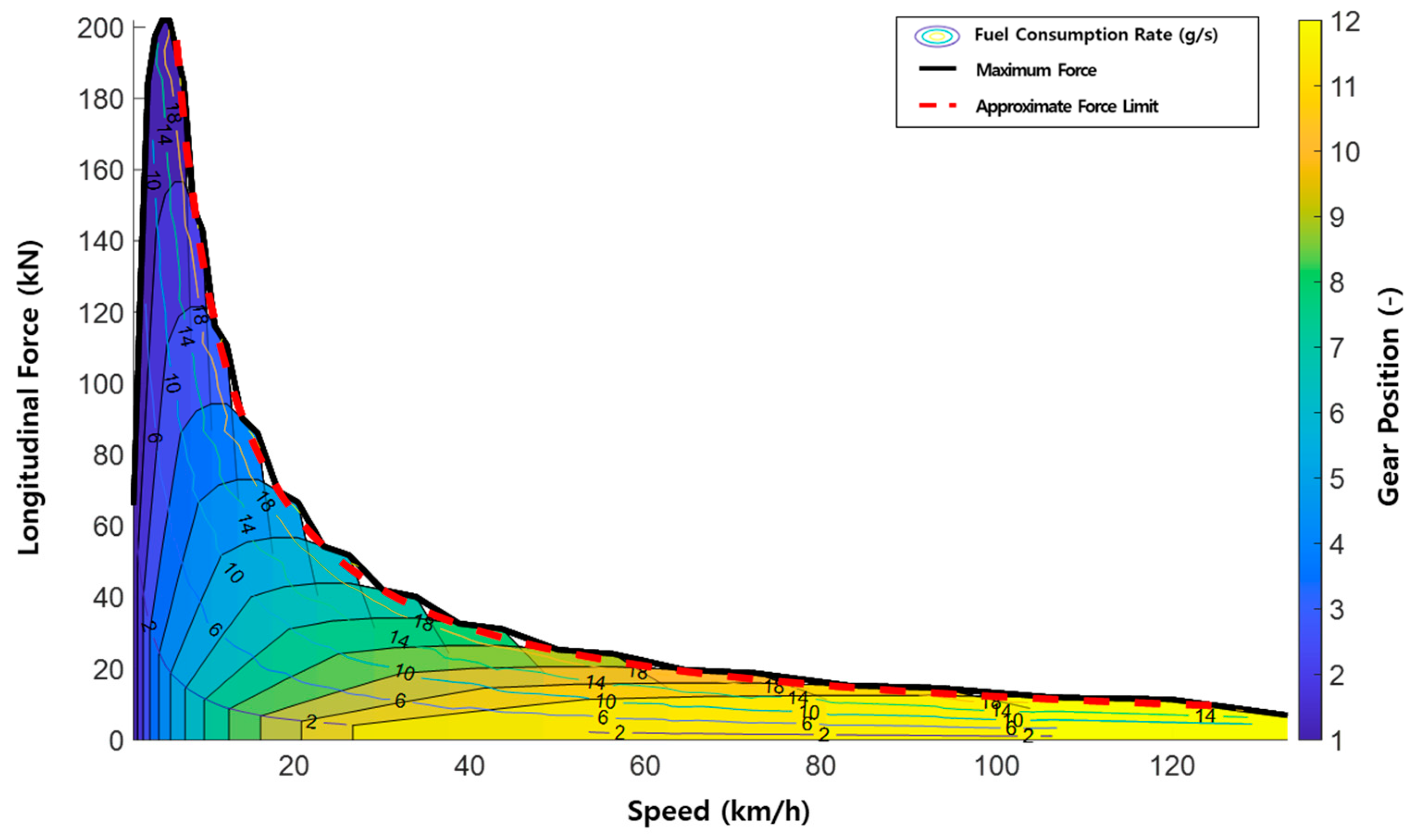
Figure 2 presents the contour plot of the fuel consumption rate over the engine operating range for the aforementioned 12-speed transmission. The colored contours represent the fuel mass rate distribution, which is directly related to the vehicle’s fuel efficiency, as a function of the vehicle speed and longitudinal force. The thick, solid black line indicates the maximum tractive force F m a x achievable by the powertrain across different gears. At each speed, F m a x is determined as the maximum tractive force achievable in each gear within the engine speed range.
The dashed red line in Figure 2 represents the approximated maximum tractive force, calculated using the following equation:
F ~ m a x v a 0 + a 1 1 v ,
where F m a x is approximated as a rational function of velocity. To determine the coefficients a 0 and a 1 of the rational function, a linear programming approach was employed [22]. The approximated F m a x thus obtained demonstrated high accuracy over a velocity range of 6–125 km/h.

2.6. Fuel Consumption Model

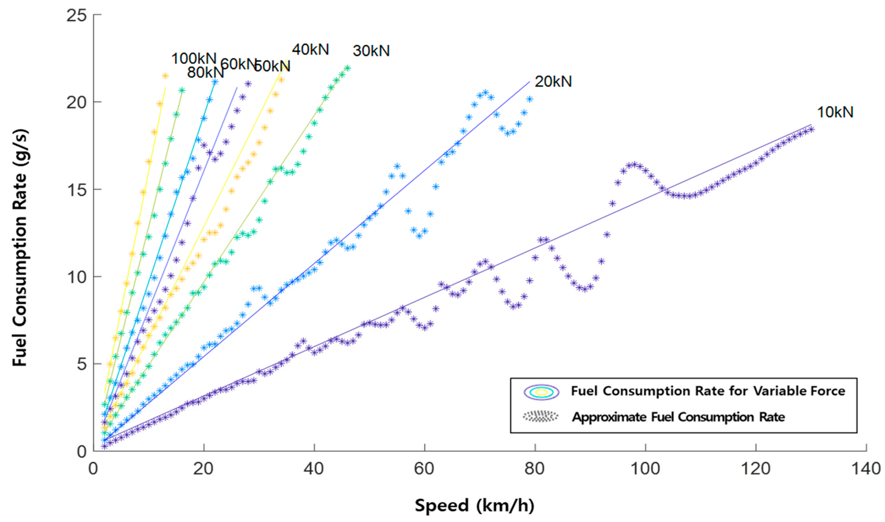
Predicting fuel consumption is essential for optimal fuel-efficient driving. Engine manufacturers typically provide fuel consumption data in the form of brake-specific fuel consumption (BSFC), which represents the mass of fuel consumed relative to the engine output per unit time. Multiplying the BSFC by the engine power yields the instantaneous fuel consumption rate. While such data are commonly utilized in the form of lookup tables, in this study, the fuel consumption rate was approximated as a polynomial function of the driving resistance force F w and vehicle speed v , as shown in Equation (8), to facilitate the formulation of the subsequent optimal control problem. Figure 3 presents the corresponding approximation results.
Q F C F w , v = b 0 + b 1 v 3 s + b 2 v s F w ( s ) ,
y A b ,           t h u s b = A + y , A = 1 v 1 3 v 1 F w , 1 1 v 2 3 v 2 F w , 2 1 v n 3 v n F w , n ,   b = b 0 ,   b 1 , b 2 T ,       y = Q s ,   1 ,   Q s , 2 ,   ,   Q s , n T .
The coefficient vector b can be determined from fuel consumption rate data using the least-squares method. In Equation (9), A + denotes the Moore–Penrose pseudoinverse of A [29].
Figure 3 demonstrates that the fuel consumption rate can be sufficiently approximated using only the first-order term of the driving force F w . The formulation employed in this study is not intended for precise calculation of absolute fuel consumption; instead, it serves as an approximation model for capturing the overall fuel consumption trend.

3. Optimal Model for Eco-Driving

3.1. Problem Formulation

The proposed global velocity profile for long-distance highway driving is designed to minimize fuel consumption while simultaneously ensuring punctuality. To this end, the cost function is defined as the cumulative fuel consumption, and a travel time constraint is imposed to guarantee on-time arrival. Additionally, capacity constraints reflecting the vehicle’s performance limits are incorporated. As shown in Equation (10), the total cumulative fuel consumption is calculated by summing the product of the fuel consumption rate and the ratio of segment distance to velocity across all road segments:
T o t a l   F u e l   C o s u m p t i o n = k = 0 N 1 Q F C F w , v k v ( k ) S ,
J = min F w , F brk k = 0 N 1 Q F C F w , E k m 2 E k S ,
subject to t ( k ) = t k + 1 t ( k ) = m 2 E k S ,
E ( k ) = E k + 1 E k = F w k + F b r k k c ~ a E k F α k S ,
m 2 v m i n 2 E k m 2 v m a x 2 ,
0 F w k F m a x E k ,
F b r k , m a x F b r k k 0 ,
t N S N v r t m a r g i n ,
t 0 = t 0 , E 0 = m v 0 2 2 .
Equation (11) represents the optimal control problem formulated in this study. The cost function in Equation (11a) divides the total driving distance into N uniform segments and quantitatively computes the cumulative fuel consumption for each segment. Here, S denotes the finely sampled distance vector, and S represents the fixed-step segment length. Based on Equation (4), by substituting the vehicle speed v in the fuel consumption function with the kinetic energy E , the cost function can be expressed in terms of the control variable F w and the state variable E . Equations (11b) and (11c) describe the state dynamics of travel time and kinetic energy, while Equations (11d)–(11f) represent the capacity constraints reflecting the vehicle’s performance limits. Equation (11g) constrains the difference between the estimated travel time at the reference speed for the remaining distance and the actual time of arrival at the final destination, while Equation (11h) specifies the initial conditions.
Furthermore, using the previously defined approximations for fuel consumption and maximum driving force, Equations (11a) and (11e) can be reformulated into Equation (12):
min F w ,   F brk k = 0 N 1 b 0 m 2 E k + 2 b 1 m E k + b 2 F w k   S ,
0 F w k a 0 + a 1 m 2 E k .

3.2. Variable-Step Spatial Segmentation

For heavy-duty commercial vehicles, rolling resistance and grade resistance constitute the largest components of the total driving resistance, rather than aerodynamic drag. Both resistances can be expressed as functions of the road slope α . Most previous studies on optimal driving strategies utilized a fixed-step segmentation approach, which involved discretizing the road into uniform segments and using the slope in each segment to calculate the driving resistance for optimal control. However, if the segment spacing is too small when using this technique, the number of control points increases excessively, significantly raising the computational cost; conversely, if the segment spacing is too large, the road geometry cannot be accurately captured, which introduces errors in the predicted driving resistance.
Thus, the segmentation method directly affects both the computational efficiency and accuracy of driving resistance prediction. In this study, a variable-step road segmentation approach was employed, which involves progressively aggregating high-resolution road slope data into larger segments. The segmentation is performed such that the cumulative squared error between the mean slope of each segment and the original sample-point slopes satisfies a predefined tolerance.

3.2.1. Notation

The following symbols are used throughout this section:
  • S = s 1 , s 2 , , s N T R N : finely sampled distance vector at 20 m intervals;
  • α = α 1 , α 2 , , α N 1 T R N 1 : slope vector between consecutive distance vectors;
  • N : number of distance sample datapoints;
  • ϵ : slope error threshold;
  • S i d x : variable-step segment index set;
  • k: current segment start index;
  • j: candidate segment end index;
  • S ^ : variable-step spatial segment set;
  • α ^ : segment-averaged slope set.

3.2.2. Error Criterion

Based on the foregoing definitions, the sum of the squared errors for a segment [k,j] is
E k , j = i = k j 1 α i α ¯ k , j 2 ,
where α ¯ k , j = 1 j k i = k j 1 α i represents the segment-averaged slope for road segment [k,j], and E k , j denotes the cumulative squared deviation of the slopes within segment [k,j] from the segment-averaged slope.

3.2.3. Algorithm

Based on the aforementioned criterion, the variable-step segmentation procedure is summarized in Algorithm 1, which presents the pseudocode for the variable-step spatial segmentation method. The tolerance parameter ϵ was empirically set to 0.001. The set of segment lengths and the corresponding segment-averaged slopes were obtained using this algorithm.
Algorithm 1: Spatial Segmentation based on Sum of Squared Errors
1: I n p u t :     S ,   α ,   N ,   ϵ
2: O u t p u t :     S ^ ,   α ^
3: k 1
4: S i d x { 1 } ▷ List of Segment Start Indices
5: w h i l e   k < N   d o
6: j k + 1
7: w h i l e   j N   d o
8: n j k
9: α ¯ 1 n i = k j 1 α i ▷ Segment-Averaged Slope
10: E i = k j 1 α i α ¯ 2 ▷ Sum of Squared Errors
11: i f   E > ϵ   t h e n ▷ End criteria
12: b r e a k
13:   else
14: j j + 1
15:   end if
16:  end while
17:   S i d x S i d x { j } ▷ Append Segment End Index
18:   k j ▷ Update k
19:end while
20: M l e n g t h S i d x 1 ▷ Number of Segments
21:for m=1 to M do
22: p S i d x m ,   q S i d x m + 1 1
23: d S ^ m S q S ( p )
24: n p , q q p + 1
25: α ^ m 1 n p , q i = p q α i
26:end for
27: S ^ c u m s u m ( d S ^ ) ▷ Cumulative Sum of Segment Distances
28:return S ^ ,   α ^

3.3. QP Reformulation

An efficient approach was devised to solve the optimal control problem defined in Equation (11) in real time. The real-time requirement for long-distance velocity planning is typically defined as a computation rate of at least 1 Hz, which allows for slower computation compared with low-level vehicle control.
The optimal control problem in Equation (11) involves numerous nonlinear terms in both the cost function and the constraints and is therefore generally solved using NLP methods. However, solving a large-scale NLP problem for long-distance highway routes spanning tens or hundreds of kilometers is impractical due to the prohibitively long computation time required. Hence, a procedure was established in this study to reformulate NLP problems into QP problems by approximating the cost function and constraints.
A QP problem is defined by a quadratic objective function and linear (affine) constraints. Linearizing or quadratically approximating the nonlinear terms in an NLP problem yields a QP formulation, enabling the solver to compute solutions efficiently using matrix operations. Equation (11) is transformed into a QP problem through the following approximation step:
The nonlinear term in Equation (12), f E = 1 E ( k ) , is linearized using a Taylor approximation. Here, the constraints are expressed as first-order linear functions, while the QP form of the cost function is retained by computing both first-order and second-order approximations.
f l i n E , E ^ = f E ^ + d f E d E E ^ E k E ^ ,
f q u a d E , E ^ = f l i n E , E ^ + 1 2 d 2 f E d E 2 E ^ E ( k ) E ^ 2 .

3.3.1. Objective Function Approximation for QP

By substituting Equation (14b) into the cost term in Equation (12a), the cost function can be expressed as shown in Equation (15):
P · = f q u a d E , E ^ b 0 m 2 + 2 b 1 m E k + b 2 F w k   : =   p 0 E 2 + p 1 E + p 2 F w + p 3 , where p 0 = b 0 2 m 2 d 2 f E d E 2 E ^ , p 1 = 2 b 1 m + b 0 m 2 d f E d E E ^ d 2 f E d E 2 E ^ E ^ , p 2 = b 2 .
Here, p 3 is a constant and is omitted from the subsequent formulation. Additionally, to transform the cost function into a QP form, all state variables must be converted into optimization variables. Based on the state dynamics in Equation (11c), the state E in the cost term can be expressed in terms of the control variable u :
E = a E E 0 + B E u C E F α , where a E = γ 0 γ 1 γ 0 γ 2 γ 1 γ 0 γ n 1 γ n 2 γ 1 γ 0 R N , γ k = 1 c a d S ^ ( k ) , C E = d S ^ 0 0 0 0 γ 1 d S ^ 0 d S ^ 1 0 0 γ 2 γ 1 d S ^ 0 γ 2 d S ^ 1 d S ^ 2 0 0 γ ( n 1 ) γ 1 d S ^ 0 γ n 1 γ ( 2 ) d S ^ 1 γ ( n 1 ) γ 3 d S ^ ( 2 ) d S ^ ( n 1 ) R N x N , B E = C E ,   C E R N x 2 N , u = F w 0 , , F w N 1 , F b r k 0 , , F b r k N 1 T R 2 N , F α = F α 0 , , F α N 1 T R N .
Finally, by substituting Equation (16) into Equation (15), the cost function is fully reformulated into a QP problem form, as shown in Equation (17):
min u 1 2 u T H u + f T u , H = 2 p 0 B E T Q s B E , f = 2 p 0 E 0 B E T Q s a E 2 p 0 B E T Q s F α C E + p 1 B E T Q s + p 2 1 1 × N ,   0 1 × N T , where Q s = d i a g d S ^ ,   d S ^ d S ^ 0 ,   d S ^ 1 , , d S ^ N 1 T .

3.3.2. Constraints Approximation for QP

Similar to the cost function, the constraints of the optimization problem must also be expressed in terms of the optimization variable u . Hence, the nonlinear inequality constraints in Equations (11d)–(11g) are transformed into linear forms suitable for a QP formulation. Accordingly, all inequality constraints can be summarized as follows:
A i n e q u b i n e q ,           w h e r e     A i n e q R 6 N + 2 × 2 N ,   b i n e q R 6 N + 2 × 1
  • Kinetic Energy Constraints
Based on Equation (16), the kinetic energy constraint in Equation (11d) can be expressed as upper and lower bounds on the energy E :
E m i n E E m a x .
  • Wheel Traction Force Constraints
Based on Equations (12b) and (14a), the constraint in Equation (11e) can be reformulated to ensure that the wheel traction force F w ( k ) at each timestep k lies within a specified range. This formulation constrains the wheel traction force to remain non-negative while not exceeding the maximum available traction force F m a x E k , which is a function of the energy state E ( k ) :
0 F w k F m a x E k ,           w h e r e     F m a x E k = a 0 + a 1 m 2   f l i n E , E ^ .
  • Braking Force Constraints
The constraints in Equation (11f) represent the physical limits of the braking system. Considering the maximum brake torque T b r k ,   m a x and wheel radius r w , Equation (11f) can be converted into a constraint on the wheel braking force F b r k ( k ) :
F b r k , m a x F b r k k 0 , w h e r e     F b r k , m a x = T b r k , m a x r w 0 .
It is assumed that both the wheel traction force and the brake force operate within the range of the vehicle’s available tire-road friction. According to [30], the friction coefficient on wet asphalt is approximately 0.45–0.6. Based on this, a ground vehicle can achieve an acceleration of about 0.45–0.6 g on a wet road. As shown in Figure 2, when the legal speed limit on highways is 50–100 km/h, this does not exceed the range of traction force that the vehicle can actually generate, and in non-emergency situations, deceleration within 0.45–0.6 g is sufficient for braking. Therefore, the constraints on both traction and braking forces can be applied directly as expressed in the above equations.
  • Final Travel Time Constraint
The final travel time constraint in Equation (11g) can be reformulated by expanding the state equations—Equations (11b) and (14a)—to ensure that the arrival time at the destination remains within the allowable tolerance t m a r g i n :
t N S ( N ) / v r t m a r g i n ,           w h e r e       t = t 0 + m 2 f l i n E ,   E ^ T d S ^ .

3.3.3. Acceleration Penalty for Ride Comfort

To enhance cargo safety and ride comfort, an acceleration penalty term E ( s ) is added to the cost function. Since acceleration can be positive or negative, it is squared to ensure a non-negative contribution before being added to the cost function. Thus, the cost function can be reformulated into a QP form.
A d d i t i o n a l   C o s t   t e r m :   k = 0 N 1 w 1 E k 2 d S ^ k = w 1 E T Q s E , where E k = E k + 1 E k S ( k ) = F w k + F b r k k c ~ a E k F α ( k ) .
E can be expressed with respect to the control input as follows:
E = a E E 0 + B E u C E F α , a E = 1 k c ~ a k | k = 1,2 , , N R N , C E i j = 1 i j c ~ a i j ,                         i j , 0 ,                                                               i < j ,                 i , j = 1 , , N , C E R N x N B E = C E ,   C E R N x 2 N .

4. Simulation Results

This section introduces the driving scenario and simulation environment used to validate the developed control logic and discusses the results from the simulation-based verification process.

4.1. Driving Scenario

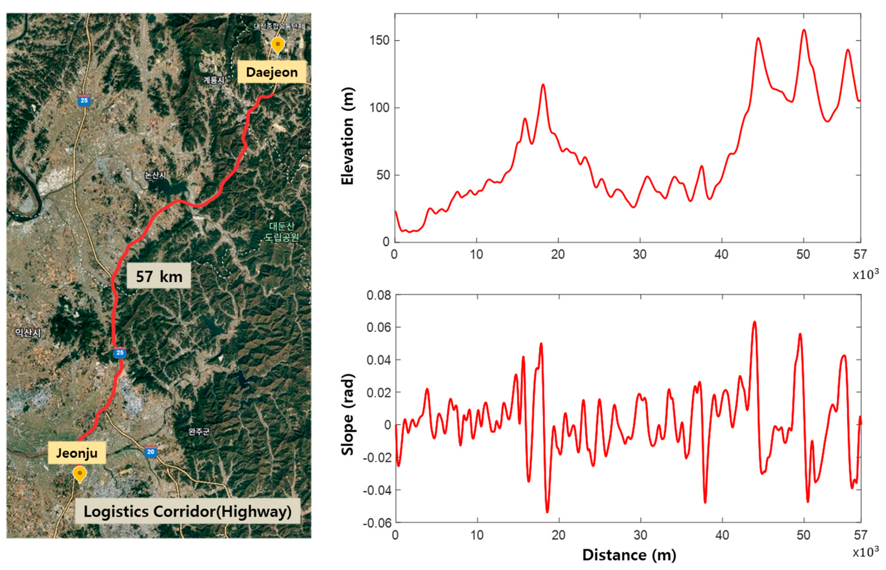
In this study, a highway section between major freight hubs, where cargo is actively transported, was selected as the test road. The location of the selected section is illustrated in Figure 4. The total length of the selected section is 57 km. During the initial 14 km of the route, the road grade changes gradually, whereafter the vehicle passes through mountainous terrain with a maximum longitudinal grade of 8%. The speed range on the road is set to 50–100 km/h, with an assumed average reference speed of 70 km/h.
Furthermore, the maximum road curvature is 0.0028 (≈360 m). By referring to the static stability factor (SSF) and the critical lateral acceleration in [31], the maximum allowable velocity is calculated to be 56 m/s. Since this value exceeds the speed limit of 100 km/h, the effect of curvature can be considered negligible. Although this represents a static limit velocity that does not account for factors such as load transfer or instantaneous lateral forces, it is valid under the assumption that no abrupt lane changes or maneuvers inducing high lateral acceleration are performed.

4.2. Comparison of Spatial Segmentation

Table 1 compares the results between the proposed variable-step spatial segmentation method, described in Section 3, and the conventional fixed-step segmentation method. For highway sections where the road geometry is continuous and the slope changes gradually, the spatial segmentation for slope approximation can be relatively coarse. Therefore, fixed step lengths of 200 m and 500 m were selected for comparative analysis.
When the entire road was divided into fixed segments of 200 m, the mean error was 0.0031 rad (0.17 ° ), which indicates a very high similarity to the actual road slope. However, the number of segments reached 285, resulting in 1712 constraints. This significantly increased the size and complexity of the optimal control problem, raising the computation time and potentially causing the interactions between the constraints to hinder numerical convergence.
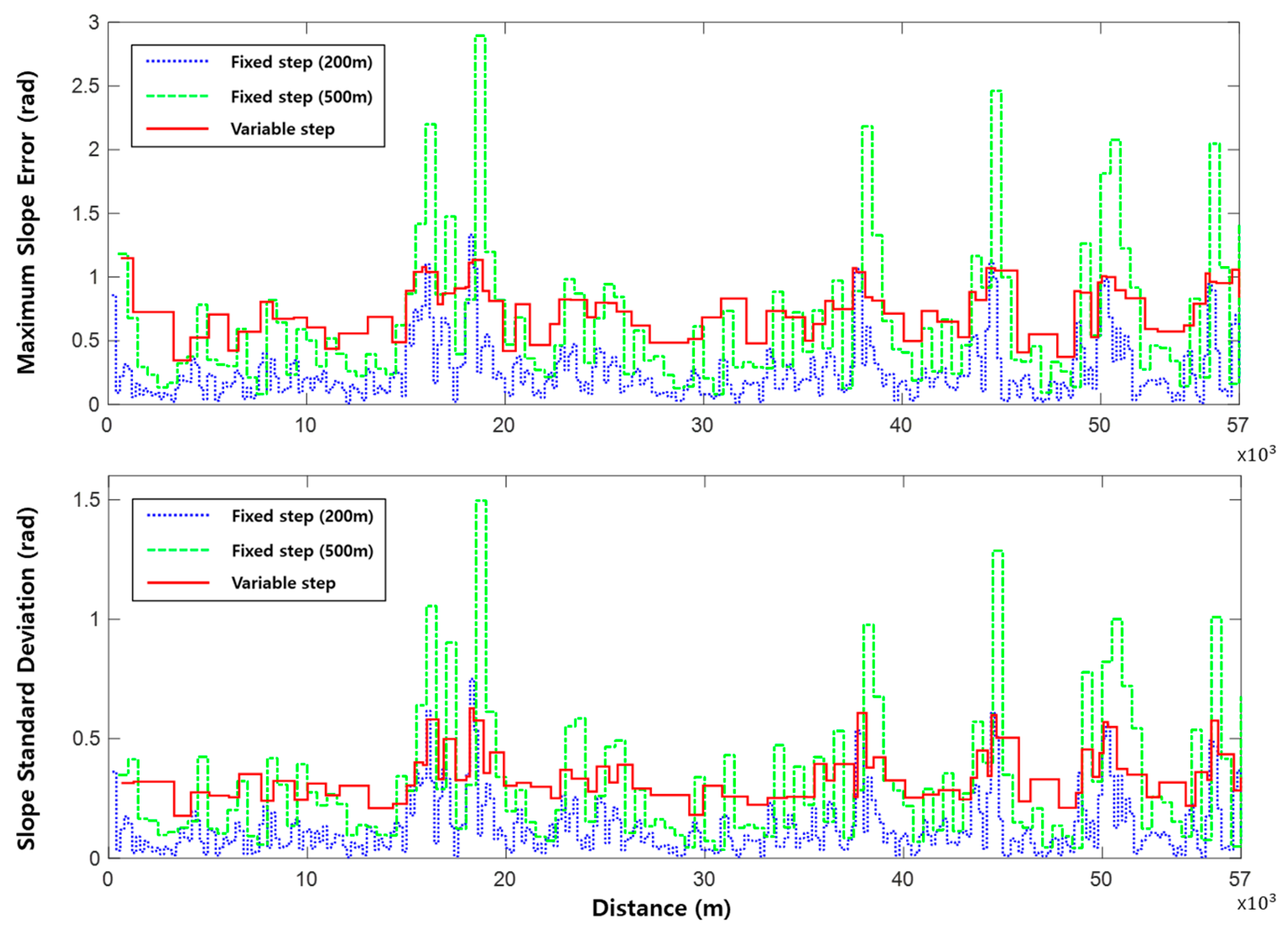
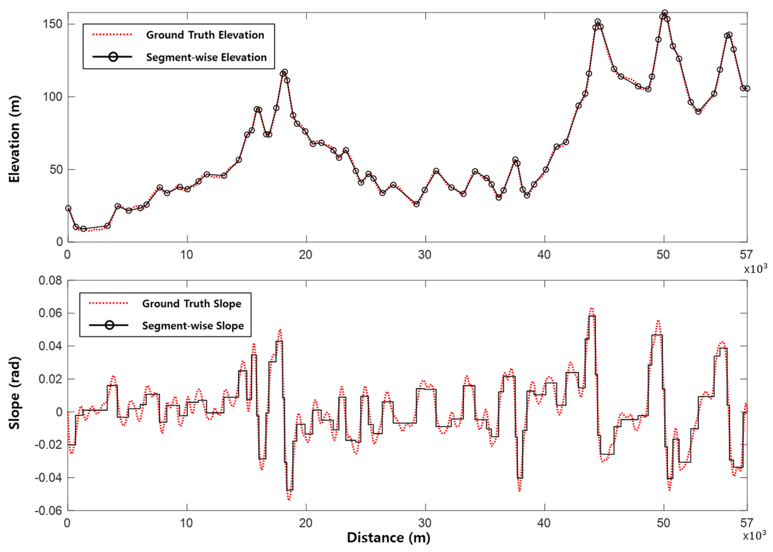
In contrast, the variable-step spatial segmentation technique produced only 83 segments and exhibited an average road-grade error of 0.0053 rad (0.3°), which was lower than the error observed with 500 m fixed-step segmentation. As shown in Figure 5, the maximum error in both fixed-step cases exceeded that of the variable-step segmentation.
Moreover, the variable-step approach exhibited stable segment-wise standard deviations, converging within a safe error range without large fluctuations. As intended in the algorithm described in Section 3, the segments were more densely distributed in regions with rapidly changing slopes while being longer in sections with gentle slopes. This can be observed in Figure 6, which compares the elevation and slope approximations between the actual road and the variably segmented road.
The reduction in the number of segments achieved using the variable-step segmentation method not only reduces the computational burden but also improves numerical stability during optimization. By adaptively allocating segment lengths based on the slope variation, the variable-step method maintains high accuracy where it is required the most while avoiding unnecessary constraints in gentle-slope regions. This balance enables faster computation as well as more efficient memory usage and better convergence properties. Hence, this approach is particularly suitable for real-time applications involving eco-driving and optimal velocity profile planning over long highway routes.

4.3. Simulation Environment

The optimal solution (velocity profile) to the defined QP problem was obtained using the primal-dual interior-point method in MATLAB 2022b. The resulting velocity profile v ( s ) was validated using the velocity profile maneuver feature in IPG TruckMaker 14.0. This feature allows precise velocity tracking by automatically applying appropriate gear shifts and drive/brake control inputs according to the target vehicle’s specifications to follow the specified velocity profile.
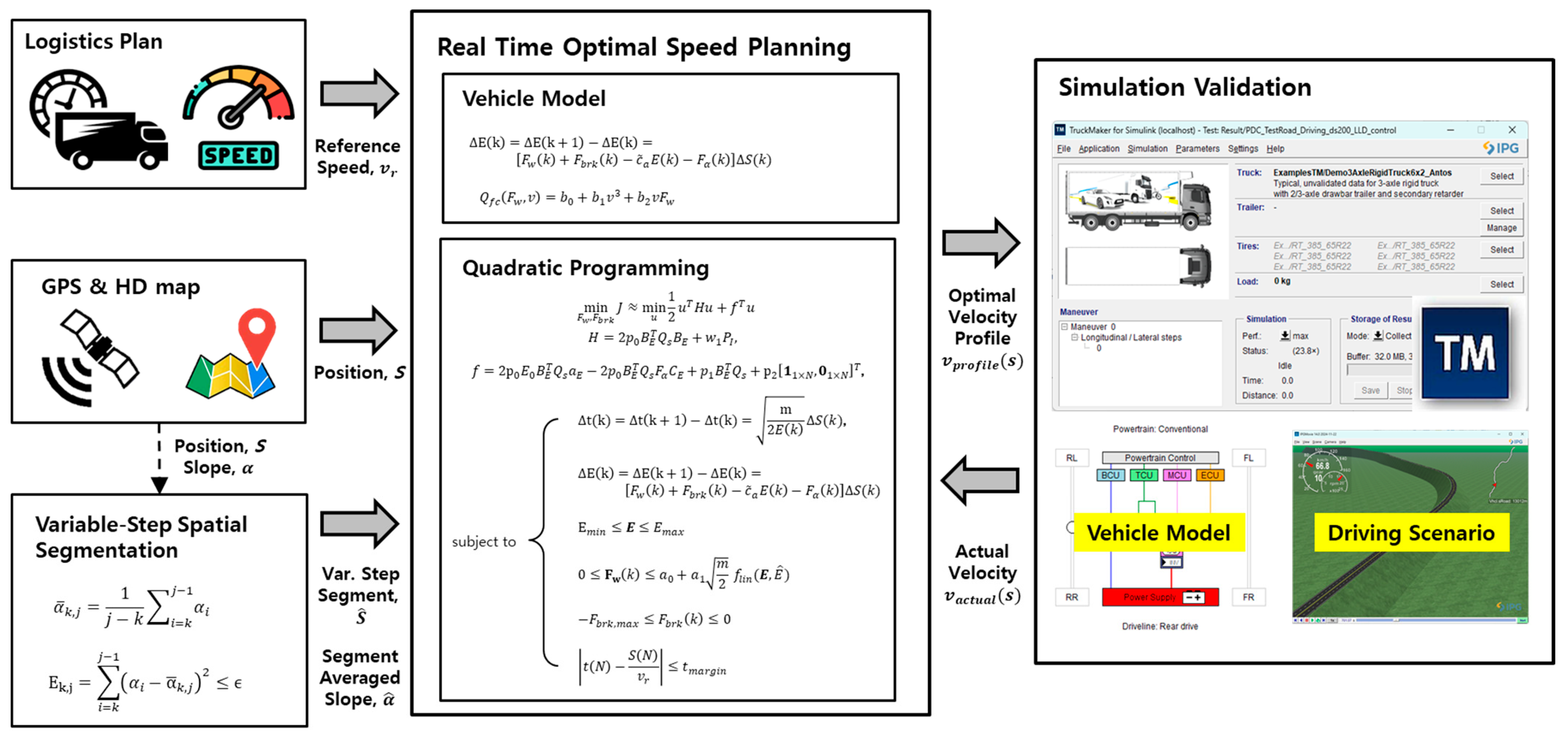
The validation was performed using a 6 × 2 cargo truck, the model and control-related parameters for which are listed in Table 2. Additionally, the scenario editor in TruckMaker was used to replicate the actual road geometry (e.g., curvature and grade) to match the defined driving scenario. The overall structure of this control and simulation environment is illustrated in Figure 7.

4.4. Simulation Results and Discussion

The accuracy of the velocity profile obtained from the QP problem using the proposed variable-step spatial segmentation algorithm was evaluated through comparisons with several reference cases. The reference cases included a benchmark DP-based velocity profile, a velocity profile based on spatial segmentation with a fixed 200 m step, and a velocity profile based on an adaptive cruise control (ACC) system set to a constant target speed of 70 km/h. The ACC was implemented in TruckMaker using the Speed Control Maneuver, which allows the vehicle to follow the specified target speed. Furthermore, to analyze the effects of vehicle load on dynamic characteristics, simulations were conducted with the truck both empty and fully loaded.

4.4.1. Results Under Curb-Weight Condition

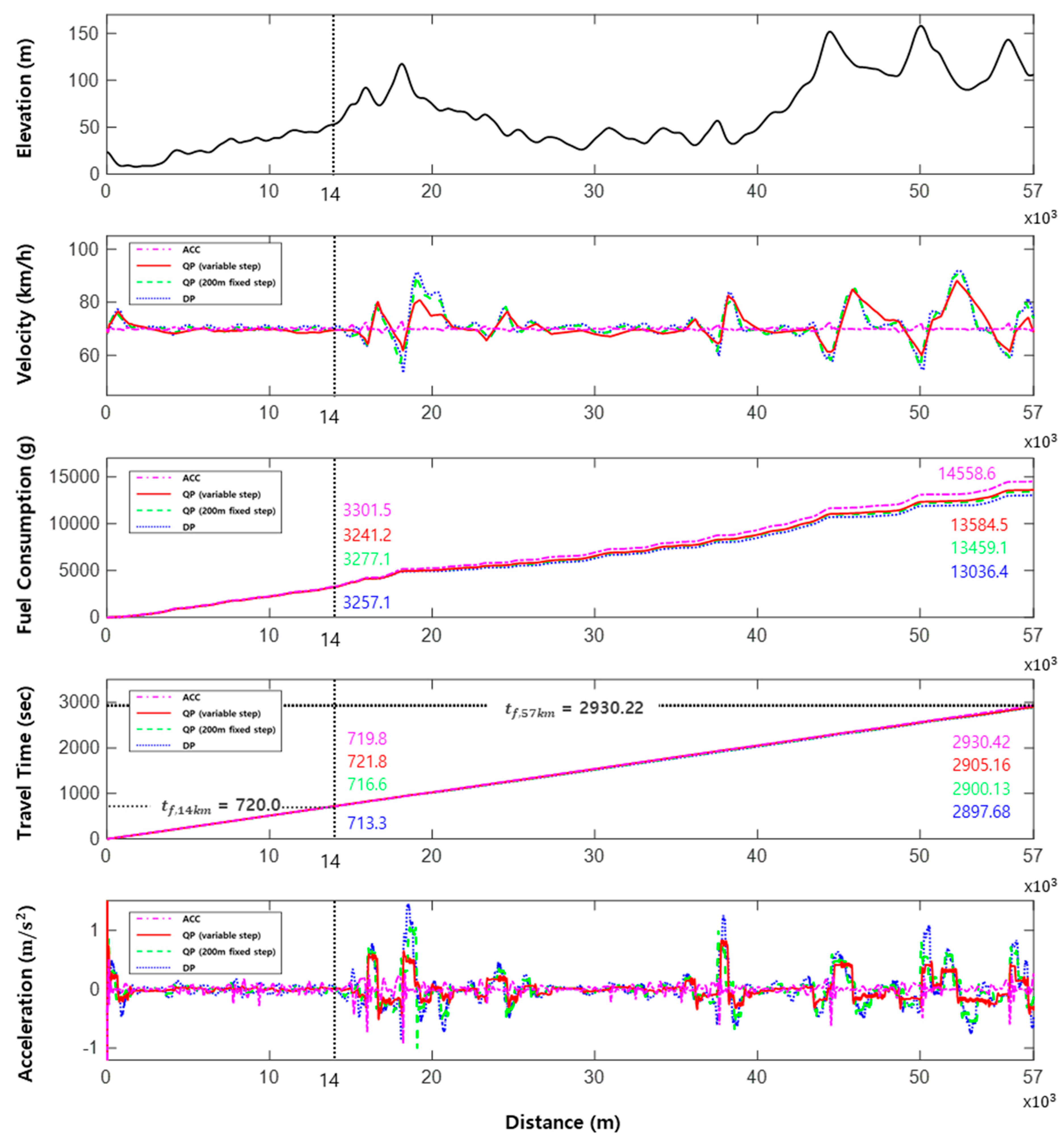
Figure 8 compares the simulation results obtained using the four specified methods for the cargo truck traveling unloaded on the test highway. The vehicle traveled on a relatively gentle slope for the first ~14 km, whereafter it encountered a steep section with a maximum longitudinal grade of 8%.
The data in Table 3 show that across the initial 14 km, all four algorithms exhibited only minor speed variations and negligible differences in fuel consumption. The variable-step QP algorithm partitioned the road based on the cumulative slope error and computed the velocity profile using the mean slope values of 16 segments, as shown in Figure 6. Consequently, it responded less sensitively to small slope changes, thus exhibiting slight deviations in average speed and travel time. However, these deviations remained within a 3% tolerance relative to the reference values and are thus not practically significant. In terms of fuel consumption, this algorithm achieved the best result, followed by the DP, fixed-step (200 m) QP, and ACC-based algorithms.
Across the entire 57 km mixed-terrain route, the differences in fuel consumption among the algorithms increased in sections with steep slopes, as shown by the corresponding graph in Figure 8. Nevertheless, all four algorithms maintained a travel time and average speed within 3% of the respective reference values. After completing the 57 km route, the total fuel savings relative to ACC were the highest for DP (>10%), while the difference between the variable-step and fixed-step (200 m) QP algorithms was negligible; this confirms the effectiveness of the variable-step spatial discretization approach. Additionally, the QP-derived velocity profile exhibited a driving behavior largely similar to that under the DP-based profile.
Regarding ride comfort, the ACC system, maintaining a constant speed of 70 km/h, produced the lowest acceleration values. The variable-step QP algorithm, which incorporates a ride comfort penalty term, displayed smaller speed fluctuations than the other two algorithms, demonstrating its effectiveness in improving ride quality.

4.4.2. Results Under Fully Loaded Condition

The effect of the optimal velocity profile was more pronounced when the truck was fully loaded than when it was unloaded. Table 3 shows that, over the initial 14 km, the deviations in average speed and travel time from the reference values were the largest for the variable-step QP algorithm, although they remained within 3%. This indicates that while the variable-step QP method prioritizes fuel efficiency, it slightly sacrifices speed consistency in the early stages of the route. Expectedly, fuel consumption was the lowest for the variable-step QP algorithm, followed by the DP, fixed-step (200 m) QP, and ACC strategies, highlighting the advantage of globally optimized velocity planning under varying load conditions.
Across the 57 km mixed-terrain route, the ACC-derived velocity profile exhibited significant speed fluctuations in steep sections. This is attributed to the increased vehicle mass under full load, which raises inertia and compromises velocity tracking in sections with abrupt grade changes. As these fluctuations lead to inefficient engine operation and frequent throttle adjustments, fuel consumption increased compared to the optimal profiles. In contrast, both fixed-step and variable-step QP-based methods effectively smoothed out the speed profile while still respecting road grade and vehicle dynamics constraints, achieving over 10% fuel savings compared to ACC. The difference in fuel efficiency between the fixed-step and variable-step QP approaches was negligible, although the variable-step method slightly reduced computation time due to the adaptive segmentation strategy.
Figure 9 confirms that the DP-based and QP-based optimal velocity profiles exhibited similar overall driving trends, suggesting that both approaches are effective in capturing the global optimal speed trajectory. Regarding acceleration, the ACC-based profile displayed the largest speed variations due to the increased vehicle mass, which may also impact ride comfort and cargo stability. In contrast, the variable-step QP strategy incorporates a ride comfort penalty term, resulting in the smallest speed fluctuations, more gradual accelerations, and better overall drivability. These characteristics imply that the variable-step QP approach not only optimizes fuel consumption but also enhances vehicle handling and safety, particularly in challenging terrain and under full-load conditions (Table 4).

4.4.3. Computation Time

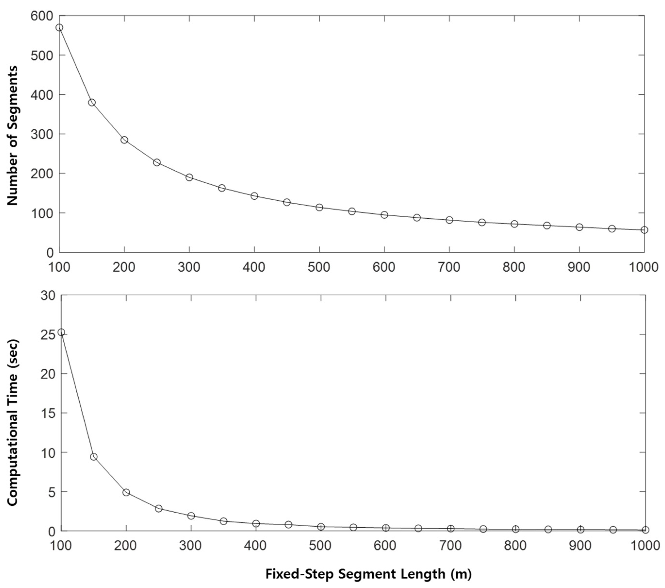
To evaluate the feasibility of generating velocity profiles in real time over global routes, the number of segments and convergence times for different fixed spatial discretization intervals were calculated, as shown in Figure 10 and Table 5. The experiments were conducted on a computer with an Intel Core i7-12700F and 64 GB of RAM. The results indicate that as the segment length decreased, the number of segments and computation time both increased exponentially.
In contrast, when using the variable-step spatial discretization method, the route was divided into only 83 segments, with a computation time of only 0.34 s. Although a direct one-to-one comparison with the fixed-step approach is not feasible, the efficiency of the proposed technique in terms of computation speed relative to the number of segments can be observed. Moreover, the experimental results demonstrate that up to 143 segments, where a calculation frequency exceeding 1 Hz was achievable, the epsilon value could be adjusted more finely to improve the accuracy of average slope estimation.

4.4.4. Experimental Result

To verify that the proposed logic operates correctly in a real driving environment rather than in an ideal PC setting, the computational performance was evaluated using an embedded computer.
The hardware configuration and operating environment are shown in Figure 11. The embedded computer used in this study is a Nuvo-5104VTC equipped with an Intel i5-6500TE processor and 32 GB of RAM. It runs on Ubuntu 18.04 with ROS Melodic. The controller model was automatically converted to C source code using the MATLAB C/C++ Coder toolbox and then deployed to the embedded computer. The embedded computer communicates with the host PC via TCP/IP.
For data acquisition and real-time logging, rostopic messages were recorded in bag files, and the results were compared with the velocity profiles generated in the PC environment.
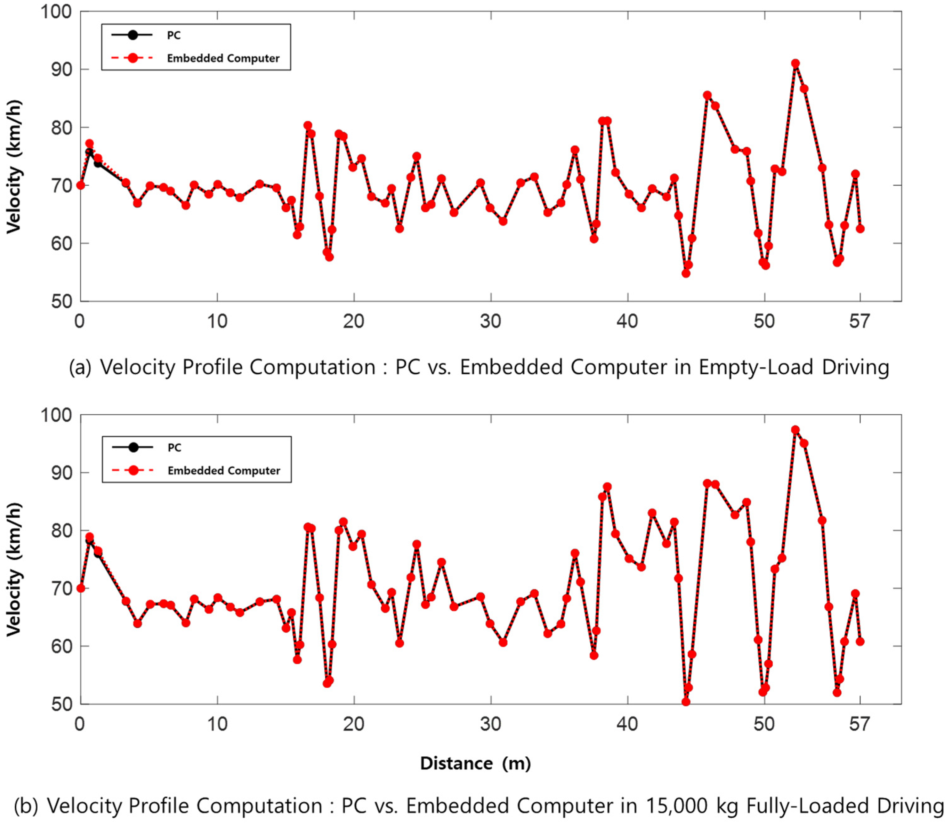
In Figure 12, the difference between the velocity profiles generated on the PC and the embedded computer is very small, and the slight discrepancies observed in certain sections are due to data type conversion during computation. On the embedded computer, fixed-point arithmetic was adopted instead of floating-point arithmetic to account for the algorithm’s high memory requirements and computational load. In contrast, the PC environment utilized double-precision floating-point data types, allowing for more precise control.
The results of running the computation under the same conditions on the embedded computer as on the PC are presented in Table 6. When the road was segmented into 100 m intervals, the algorithm failed to execute on the embedded computer due to insufficient memory space. As the number of segments increased, it was observed that the computation time on the embedded computer became longer than on the PC because of memory allocation and computational load. When running the logic on the embedded computer, the number of segments in the variable-step spatial segmentation can be adjusted using the epsilon parameter so that the resulting number of segments matches that of the fixed-step segmentation with 114 segments. A comparison of the computation times in the two environments confirmed that real-time performance can still be achieved on the embedded computer.

5. Conclusions

This paper presents a real-time velocity profile optimization framework for eco-driving of heavy-duty trucks, which incorporates a variable-step spatial segmentation method and a QP formulation. A longitudinal dynamic model of the target vehicle, including the powertrain, vehicle dynamics, and fuel consumption, was developed to accurately capture the vehicle’s behavior over varying road slopes.
The proposed variable-step spatial segmentation technique effectively reduced the number of road segments required for slope approximation, thereby delivering a significant reduction in computation time while still generating highly accurate velocity profiles. Compared with fixed-step segmentation methods, the variable-step approach achieved comparable or better performance with fewer segments, demonstrating its computational efficiency and suitability for real-time applications.
Simulation results under both unloaded and fully loaded driving showed that the QP-based optimal velocity profiles closely matched the reference DP profiles in terms of speed and travel time while achieving notable fuel savings. Specifically, over a 57 km mixed-terrain route, the QP-based methods reduced fuel consumption by more than 10% compared with a constant-speed ACC system. By incorporating an acceleration penalty term into the cost function, the variable-step QP approach reduced speed fluctuations, thus enhancing ride comfort further.
Overall, the findings of this study demonstrate that the proposed variable-step QP framework represents a practical and computationally efficient approach to real-time eco-driving optimization, balancing fuel efficiency, travel time, and ride comfort. In addition, this framework has the potential to generate broader economic, environmental, and societal benefits. By reducing fuel consumption in both empty and fully loaded scenarios, it reduces operating costs and CO2 emissions simultaneously, contributing to enhanced sustainability. Improved schedule adherence and reduced speed fluctuations can also enhance cargo safety and service reliability, making the approach highly attractive for large-scale deployment in freight transportation.
Furthermore, a comparative analysis between PC and embedded computer implementations confirmed that the proposed algorithm maintains real-time performance even under the computational and memory constraints of the embedded system. This finding demonstrates the feasibility of deploying the framework in real-world in-vehicle applications without compromising its computational efficiency or control accuracy.
Future work could extend this framework to incorporate traffic interactions, adaptive speed limits, and predictive control strategies for even more realistic scenarios and greater robustness.

Author Contributions

Conceptualization, J.Y. (Jaeyeon Yoo); methodology, J.Y. (Jaeyeon Yoo) and Y.H.; software and validation, J.Y. (Jaeyeon Yoo), J.K. and Y.H.; investigation and data curation, J.Y. (Jaeyeon Yoo) and S.M.; writing—original draft preparation, J.Y. (Jaeyeon Yoo); writing—review and editing, J.Y. (Jinwoo Yoo); visualization, J.Y. (Jaeyeon Yoo); supervision, J.Y. (Jinwoo Yoo). All authors have read and agreed to the published version of the manuscript.

Funding

This work was supported by the National Research Foundation of Korea (NRF) grant funded by the Korea government (MSIT) (No. NRF-RS-2021-NR060086).

Institutional Review Board Statement

Not applicable.

Informed Consent Statement

Not applicable.

Data Availability Statement

The data presented in this study are available on request from the corresponding author. The data are not publicly available due to privacy restrictions.

Conflicts of Interest

The authors declare no conflicts of interest.

References

  1. IPCC Sixth Assessment Report. Available online: https://www.ipcc.ch/report/ar6/wg3/ (accessed on 31 August 2025).
  2. International Energy Agency (IEA). Trucks and Buses. Available online: https://www.iea.org/energy-system/transport/trucks-and-buses (accessed on 31 August 2025).
  3. Trucksales. Mercedes Benz Predictive Powertrain Control (PPC) Review. Available online: https://www.trucksales.com.au/editorial/details/mercedes-benz-predictive-powertrain-control-ppc-review-145985/ (accessed on 31 August 2025).
  4. Held, M. Fuel-Efficient Look-Ahead Control for Heavy-duty Vehicles with Varying Velocity Demands; KTH Royal Institute of Technology: Stockholm, Sweden, 2020. [Google Scholar]
  5. Daimler Truck AG. Available online: https://www.daimlertruck.com/en/newsroom/pressrelease/predictive-powertrain-control-ppc-10-questions-and-answers-about-the-predictive-cruise-control-from-mercedes-benz-trucks-46682406 (accessed on 31 August 2025).
  6. Federal Highway Administration (FHWA), U.S. Department of Transportation. Available online: https://www.federalregister.gov/documents/2017/01/18/2017-00681/national-performance-management-measures-assessing-performance-of-the-national-highway-system (accessed on 31 August 2025).
  7. FDOT. Travel Time Reliability 101. Available online: https://fdotwww.blob.core.windows.net/sitefinity/docs/default-source/planning/fto/reliability/reliability-101.pdf (accessed on 31 August 2025).
  8. Federal Highway Administration (FHWA), U.S. Department of Transportation. Available online: https://ops.fhwa.dot.gov/publications/tt_reliability/brochure/ (accessed on 31 August 2025).
  9. Federal Motor Carrier Safety Administration (FMCSA), U.S. Department of Transportation. Available online: https://www.fmcsa.dot.gov/sites/fmcsa.dot.gov/files/docs/Development_of_a_North_American_Standard_for_Protection_Against_Shifting_and_Falling_Cargo_508CLN.pdf (accessed on 31 August 2025).
  10. Federal Motor Carrier Safety Administration (FMCSA), U.S. Department of Transportation. Available online: https://www.federalregister.gov/documents/2000/12/18/00-31919/development-of-a-north-american-standard-for-protection-against-shifting-and-falling-cargo (accessed on 31 August 2025).
  11. Xu, C.; Geyer, S.; Fathy, H.K. Formulation and comparison of two real-time predictive gear shift algorithms for connected/automated heavy-duty vehicles. IEEE Trans. Veh. Technol. 2019, 68, 7498–7510. [Google Scholar] [CrossRef]
  12. Li, S.; Yang, L.; Gao, Z. Efficient real-time control design for automatic train regulation of metro loop lines. IEEE Trans. Intell. Transp. Syst. 2018, 20, 485–496. [Google Scholar] [CrossRef]
  13. Zhang, J.; Jin, H. Optimized calculation of the economic speed profile for slope driving: Based on iterative dynamic programming. IEEE Trans. Intell. Transp. Syst. 2020, 23, 3313–3323. [Google Scholar] [CrossRef]
  14. Honda, K.; Yonetani, R.; Nishimura, M.; Kozuno, T. When to replan? An adaptive replanning strategy for autonomous navigation using deep reinforcement learning. In Proceedings of the 2024 IEEE International Conference on Robotics and Automation (ICRA), Yokohama, Japan, 13–17 May 2024; IEEE: Yokohama, Japan, 2024; pp. 6650–6656. [Google Scholar]
  15. Lee, Y.; Lee, D.Y.; Lee, S.H.; Kim, Y. A comparative study on model predictive control design for highway car-following scenarios: Space-domain and time-domain model. IEEE Access 2021, 9, 162291–162305. [Google Scholar]
  16. Bellman, R. Dynamic Programming; Princeton University Press: Princeton, NJ, USA, 1957; p. 39. [Google Scholar]
  17. Hellström, E.; Ivarsson, M.; Åslund, J.; Nielsen, L. Look-ahead control for heavy trucks to minimize trip time and fuel consumption. Control. Eng. Pract. 2009, 17, 245–254. [Google Scholar]
  18. Hellström, E. Look-Ahead Control of Heavy Trucks Utilizing Road Topography; Linkopings Universitet: Linköping, Sweden, 2007. [Google Scholar]
  19. Pulvirenti, L.; Tresca, L.; Rolando, L.; Millo, F. Eco-driving optimization based on variable grid dynamic programming and vehicle connectivity in a real-world scenario. Energies 2023, 16, 4121. [Google Scholar]
  20. Shiledar, A.; Gupta, S.; Spano, M.; Villani, M.; Canova, M.; Rizzoni, G. Real-time eco-driving of a connected and automated fuel cell electric truck using approximate dynamic programming. In Proceedings of the 2024 American Control Conference (ACC), Toronto, ON, Canada, 10–12 July 2024; IEEE: Toronto, ON, Canada, 2024; pp. 2989–2994. [Google Scholar]
  21. Spano, M.; Shiledar, A.; Gupta, S.; Villani, M.; Misul, D.; Canova, M.; Rizzoni, G. Performance Evaluation of an Eco-Driving Controller for Fuel Cell Electric Trucks in Real-World Driving conditions; SAE Technical Paper; SAE: Warrendale, PA, USA, 2024. [Google Scholar]
  22. Hamednia, A.; Murgovski, N.; Fredriksson, J. Predictive velocity control in a hilly terrain over a long look-ahead horizon. IFAC-Pap. 2018, 51, 485–492. [Google Scholar]
  23. Hamednia, A.; Sharma, N.K.; Murgovski, N.; Fredriksson, J. Computationally efficient algorithm for eco-driving over long look-ahead horizons. IEEE Trans. Intell. Transp. Syst. 2021, 23, 6556–6570. [Google Scholar] [CrossRef]
  24. Zhang, Y.; Qu, X.; Tong, L. Optimal eco-driving control of autonomous and electric trucks in adaptation to highway topography: Energy minimization and battery life extension. IEEE Trans. Transp. Electrif. 2022, 8, 2149–2163. [Google Scholar]
  25. Li, X.; Lv, T.; Yue, H.; Liu, S.; Na, X.; Chen, H.; Gao, B. Predictive cruise control algorithm design for commercial vehicle energy saving based on quadratic programming. In International Conference on Energy Storage and Intelligent Vehicles; Springer: Berlin/Heidelberg, Germany, 2022; pp. 1076–1088. [Google Scholar]
  26. Watling, D.P.; Connors, R.D.; Chen, H. Fuel-optimal truck path and speed profile in dynamic conditions: An exact algorithm. Eur. J. Oper. Res. 2023, 306, 1456–1472. [Google Scholar] [CrossRef]
  27. Shimizu, Y.; Horibe, T.; Watanabe, F.; Kato, S. Jerk constrained velocity planning for an autonomous vehicle: Linear programming approach. In Proceedings of the 2022 International Conference on Robotics and Automation (ICRA), Philadelphia, PA, USA, 23–27 May 2022; IEEE: Philadelphia, PA, USA, 2022; pp. 5814–5820. [Google Scholar]
  28. Koch, A.; Nicoletti, L.; Herrmann, T.; Lienkamp, M. Implementation and analyses of an eco-driving algorithm for different battery electric powertrain topologies based on a split loss integration approach. Energies 2022, 15, 5396. [Google Scholar] [CrossRef]
  29. Albert, A. Regression and the Moore–Penrose Pseudoinverse. In Mathematics in Science and Engineering; Academic Press: New York, NY, USA, 1972; Volume 94. [Google Scholar]
  30. Popp, K.; Schiehlen, W. Ground Vehicle Dynamics; Springer Science & Business Media: Berlin/Heidelberg, Germany, 2010. [Google Scholar]
  31. Rajamani, R. Vehicle Dynamics and Control; Springer: New York, NY, USA, 2006. [Google Scholar]
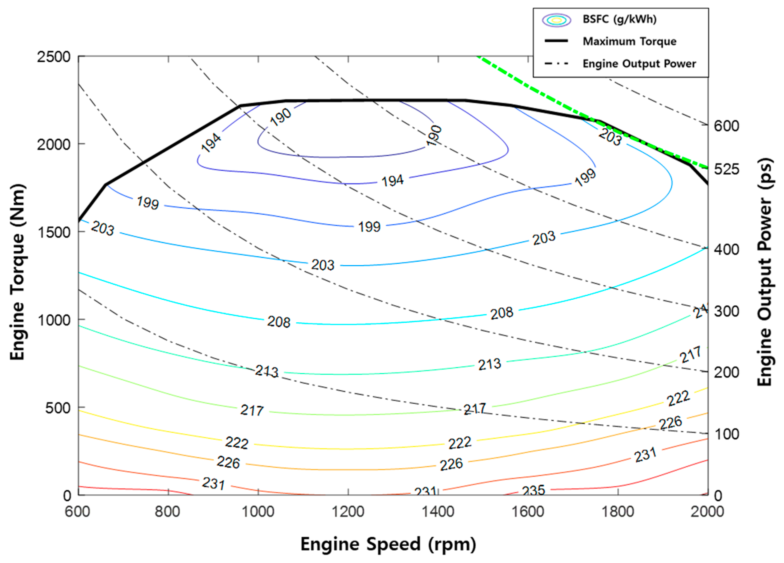
Figure 1. Static characteristic curve of target engine.
Applsci 15 10811 g001
Figure 2. Fuel consumption rate contours with respect to longitudinal force, vehicle speed, and maximum longitudinal force.
Applsci 15 10811 g002
Figure 3. Fuel consumption rates approximated for various vehicle velocities and longitudinal forces.
Applsci 15 10811 g003
Figure 4. Real-world highway with corresponding elevation and slope profiles.
Applsci 15 10811 g004
Figure 5. Maximum slope errors and standard deviations for different segmentation methods.
Applsci 15 10811 g005
Figure 6. Segment-wise approximation of elevation and slope relative to actual road profile.
Applsci 15 10811 g006
Figure 7. Control architecture and simulation environment for proposed global velocity profile generation method.
Applsci 15 10811 g007
Figure 8. Simulation results under curb-weight condition.
Applsci 15 10811 g008
Figure 9. Simulation results under fully loaded condition.
Applsci 15 10811 g009
Figure 10. Number of segments and computation time with respect to segment length.
Applsci 15 10811 g010
Figure 11. Embedded control system architecture based on PC and embedded computer communication.
Applsci 15 10811 g011
Figure 12. Velocity profile computation between PC and embedded computer.
Applsci 15 10811 g012
Table 1. Comparison between variable-step and fixed-step segmentation methods.
Segmentation MethodSegment CountConstraint CountRMSE (Rad)
Fixed step (200 m)28517120.0031
Fixed step (500 m)1146860.0072
Variable step835000.0053
Table 2. Parameters of vehicle model and controller.
CategorySymbolParameterValue
Vehicle
parameters
mMass25,200 kg
gGravitational acceleration 9.81   m / s 2
ρ a Air density 1.20   k g / m 3
C d Drag coefficient0.41
A f Frontal area 10.2   m 2
C r Rolling coefficient0.00939
r w Wheel radius0.51 m
l w Track width2.6 m
hHeight of the c.g.1.435 m
Model
parameters
ϵ Slope error threshold0.001
t m a r g i n On-time margin3%
v m i n Minimum velocity50 km/h
v m a x Maximum velocity100 km/h
v r Reference velocity70 km/h
w 1 Penalty 1 (ride comfort)10
Table 3. Performance comparison under curb-weight condition.
TerrainAlgorithmAverage
Velocity (km/h)
t f (s)Fuel Consumption Rate (L/100 km)Fuel-Saving Rate (%)
PlainACC70.02−0.229.48
QP (variable step)69.831.828.941.83
QP (200 m fixed step)70.33−3.429.260.74
DP70.65−6.729.081.34
Mixed
(plain + hilly)
ACC70.000.231.93
QP (variable step)70.61−25.0629.796.69
QP (200 m fixed step)70.73−30.0929.517.55
DP70.79−32.5428.5810.45
Table 4. Performance comparison under fully loaded condition.
TerrainAlgorithmAverage
Velocity (km/h)
t f (s) Fuel Consumption Rate (L/100 km)Fuel-Saving Rate (%)
PlainACC70.02−0.240.98
QP (variable step)68.201939.523.58
QP (200 m fixed step)69.732.840.122.11
DP69.861.439.962.50
Mixed
(plain + hilly)
ACC69.951.9844.99
QP (variable step)70.26−10.7240.4810.00
QP (200 m fixed step)70.45−18.4240.4210.16
DP70.46−19.1238.6913.99
Table 5. Comparison of segment count and computation time with respect to segment length.
Segment Length (m)Segment CountComputation Time (s)
10057025.27
2002854.90
3001901.92
4001430.93
5001140.53
600950.39
700820.29
800720.22
900640.16
1000570.13
Table 6. Comparison of computation time between PC and embedded computer.
Segment
Length (m)
Segment
Count
Computation Time (s)
PCEmbedded Computer
10057025.27-
2002854.9014.38
3001901.924.23
4001430.931.97
5001140.530.98
600950.390.62
700820.290.37
800720.220.26
900640.160.19
1000570.130.13
Disclaimer/Publisher’s Note: The statements, opinions and data contained in all publications are solely those of the individual author(s) and contributor(s) and not of MDPI and/or the editor(s). MDPI and/or the editor(s) disclaim responsibility for any injury to people or property resulting from any ideas, methods, instructions or products referred to in the content.