Article

ProposalLaneNet: Sparse High-Quality Proposal-Driven Efficient Lane Detection

1
Key Laboratory of Urban Land Resources Monitoring and Simulation, Ministry of Natural Resources, Shenzhen 518034, China
2
School of Computer Science, China University of Geosciences, Wuhan 430078, China
3
School of Geography and Information Engineering, China University of Geosciences, Wuhan 430078, China
*
Author to whom correspondence should be addressed.
Appl. Sci. 2025, 15(19), 10803; https://doi.org/10.3390/app151910803
Submission received: 25 August 2025 / Revised: 19 September 2025 / Accepted: 25 September 2025 / Published: 8 October 2025

Abstract

Lane detection is one of the key technologies for local map construction, and it is also a challenging task in intelligent driving, where various computer vision-based methods have been applied to address this issue. However, these methods often suffer from redundancy issues due to the sparse and narrow structure of the lane lines, and full generalization to lane detection needs more effort. To solve these problems, we propose a stepwise positive guidance strategy that utilizes the visually presented lane structure characteristics, which are inspired by the reference points in the DETR-Family methods. This strategy guides the network detection from the reference points to the reference lanes, improving the accuracy of the detection process. Moreover, we propose a new multi-scale feature fusion strategy that directly performs feature fusion on high-quality proposals. This approach differs from traditional object detection models using the Feature Pyramid Network (FPN). It fully uses the sparsity of lanes and reduces the network’s redundant computation. We proposed ProposalLaneNet, which takes full advantage of the lanes’ structure and sparse distribution characteristics. Significant improvements in speed and accuracy have been achieved by our method, enabling it to reach the state-of-the-art performance on the popular datasets CULane and TuSimple. Our method can be used as a new detection paradigm for lane detection.

1. Introduction

Lanes provide essential visual information for both human perception and self-driving systems, playing a crucial role in the composition of road scenes. Lane detection is not only a key technology for autonomous driving but also a vital component in the construction of local high-definition maps (HD Maps).
Thanks to the rapid development of deep learning technology over the last few years, many remarkable vision algorithms have emerged to solve the lane detection problem. This progress has brought significant advancements to the field and provided a constant source of innovation for local map construction technology, thus expanding its potential applications. Lane detection is a vital component of autonomous driving and requires a lightweight network with low computational cost [1]. Furthermore, due to the elongated structure of lane lines, the network must handle low-level road semantic information while ensuring lightweight performance. In addition, given the complexity of road scenes, the network must also be capable of processing scenarios with limited visual information, such as rainy weather, foggy weather, intense light, vehicle occlusion, light-colored lane markings, etc. This requires the network to possess sufficient high-level semantic information while retaining low-level semantic information. Therefore, this task requires a balance among high-level semantic information, low-level semantic information, and model light-weighting [2,3,4].
Lane detection algorithms are broadly classified into two categories: segmentation-based methods and detection-based methods. Initially, the classic technique of semantic segmentation was used for lane detection. Given the relatively narrow structure of lane lines, it is necessary to utilize low-level semantic information while maintaining low computational costs and addressing latency issues. To address this issue, methods such as feature-grid segmentation [1,3,5] and detection-based [2,4,6,7,8] approaches have been developed for lane detection. Based on the linear structure of lane lines, the two major approaches have been developed into keypoint-based, proposal-based, parametric curve modeling, and so on. However, detecting lane lines in challenging scenarios without visual information requires both low-level and high-level semantic information. Therefore, there is a trend toward using multi-layer rather than single-layer features. Examples of existing algorithms that reflect this trend include CondLaneNet [3], GANet [9], CLRNet [4], and BSNet [10]. These algorithms rely on the FPN [11], a feature pyramid structure for traditional object detection, which is used to enhance features. However, is the structure of the FPN truly indispensable for lane tasks? Commonly used backbones like ResNet are originally layered structures, but the pixel proportion of lane lines is minimal compared to the whole image features. As a result, these element-wise operations on all features introduce significant redundancy, thereby increasing inference time. Multi-scale information is all that is required for lane detection. Thus, instead of the FPN, a traditional object detection module, multi-scale feature fusion modules specifically tailored for lane lines would be more effective.
Inspired by PETDet [12], we propose a new method that relies on a highly efficient and reliable proposal. With the superior quality of our proposal features, we no longer require using the FPN structure. However, we do not use element-level operations in the FPN structure, but our approach still borrows from the classical multi-scale idea. We propose a new multi-scale feature fusion module that directly performs feature fusion on high-quality proposals. This approach differs from traditional object detection models that use the FPN. It fully uses the sparsity of lanes and reduces the network’s redundant computation. In addition, we do not use the operation of equal weight summation of multi-layer features in the FPN structure. We propose a new adaptive multi-scale feature fusion module, and the fusion mechanism of our module is entirely dependent on the image features.
In addition, LaneATT and CLRNet use a combination of proposal-based and anchor-based methods and rely on expert knowledge for anchor-line initialization. The difference is that LaneATT [7] directly samples features for numerous line anchors to obtain proposals, which are used to predict the offsets relative to the initialized line anchors. Meanwhile, CLRNet [4], inspired by Sparse-RCNN [13] and Cascade-RCNN [14], draws on the idea of learnable anchors based on the original strategy by updating the starting point as well as the angle of the starting point through the attention and fully connected layers, and it generates a straight line using the updated starting point information, which is finally used for sampling to generate the proposal. Although these methods have been the most effective in the past, they tend to generate low-quality proposals for very specific and flexible targets such as lane lines. Achieving better accuracy for the network requires tight control of the positive and negative sample balance. In essence, there is still a mechanical use of object detection methods. The complex structure of the lanes is not adequately considered, resulting in inflexible reference lines and redundant network computations. To solve this problem, inspired by the idea of relative coordinate regression in Conditional DETR [15], we propose a stepwise forward guidance detection strategy for the narrow and long lane structure, extending the idea of reference points to a two-stage forward reference strategy: reference starting point to reference lane. Our reference points and reference lanes are derived from the image information, and compared with the initial straight line guided by the starting point, our reference lanes are more flexible and more suitable for the actual situation of the lane.
Our prediction is wholly based on the image features. It requires minimal prior knowledge from experts and does not need to rely on the FPN and cascading strategies to make up for the irrationality of the initial proposal. Our method proved effective on the CULane [16] dataset. The experimental results show that our method can reach state-of-the-art performance. The main contributions of the method can be summarized as follows:
We make full use of the narrow and diverse structure of lane lines and propose a novel detection strategy: stepwise forward guidance detection through a reference starting point to a reference lane. Compared with the traditional starting point guidance, the reference generated by this strategy is more flexible and more consistent with the actual situation of the lane.
For the first time, we propose a novel strategy to remove element-level operations in the FPN structure, which fully uses the sparsity of lanes and reduces the network’s redundant computation.
To the best of our knowledge, this marks the first application of attention results as fusion feature weights for integrating multi-layer features in lane detection, effectively substituting the conventional 1:1 mechanical proportional fusion in the FPN structure. This method is more rational and practical, leveraging the inherent image features for fusion.
Experiments show that our method achieves just the right balance of speed and accuracy on top of CULane and TuSimple datasets; these datasets are widely used in the field of lane detection, realizing the state of the art in speed and accuracy.

2. Related Work

2.1. Segmentation-Based Methods

2.1.1. Traditional Semantic Segmentation

In this method, each pixel is classified into two or more categories, and the final result is obtained by post-processing combined with the auxiliary segmentation map. Since the receptive field of semantic segmentation is limited, some feature fusion is generally carried out. For example, SCNN [16], the algorithm that won first place in the TuSimple competition, adds rows and columns of features to perform feature fusion to make up for features without visual information. However, due to excessive computing costs, real-time performance problems exist. Therefore, RESA [17] made the Spatial-CNN into a parallel structure, which changed the complexity from O ( N ) to O ( l o g N ) , but the speed is still not fast in the present time.

2.1.2. Grid Semantic Segmentation

This method usually carries out an extreme downsampling of image features to obtain feature grids and classifies feature grids at the element level, thus greatly reducing the amount of computation. This method still needs to assist in segmenting a piece of image for post-processing [1,3,5]. Theoretically, the lane width is not much different from the downsampling width, and the accuracy is not too bad. Although the latency of this method satisfies the requirements, it is fed directly into the MLP, resulting in a very large number of model parameters and requiring high graphics memory.

2.1.3. Instance Segmentation

Typically, the above method employs multi-classification, assigning each lane to a fixed category. LaneNet [18] addresses the issue of a fixed number of lanes by using clustering techniques. LaneAF [19] proposed affinity to solve this problem, but the computational cost was still high. CondLaneNet [3] is a method that combines Grid Semantic Segmentation with Instance Segmentation. The heat map detects the starting point of lane lines, and then the dynamic convolution method solves the problem of instance ambiguity and calculation cost based on the starting point. Additional offset prediction is made to compensate for the error caused by downsampling, but starting point recognition can be difficult in complex scenes.

2.2. Detection-Based Methods

2.2.1. Keypoint-Based Lane Detection

This class of methods is mainly based on heat map detection, where lanes are transformed into a set of points, and lane lines are predicted by constructing a heat map of lane point sets via Gaussian functions, which also need to face the instance ambiguity problem. In addition to heat map predicting key points of lanes, PINet [20] additionally predicts offsets, using post-clustering to distinguish lane instances. FOLOLane [21] predicts local key points and refines the location by the offsets of neighboring key points. Based on keypoint detection, GANet [9] added the distinction of a key point association starting point to distinguish lane instances. These methods require inefficient post-processing, and the results are highly dependent on image resolution.

2.2.2. Curve-Based Lane Detection

This method uses expressions of parametric curves instead of bounding box coordinates for lane detection, usually without post-processing. Firstly, it is PolyLaneNet [8] that directly outputs cubic curves using the backbone of a CNN, which has a straightforward structure and, therefore, slightly lower accuracy. Subsequently, LSTR [22], inspired by DETR, added the transformer structure after the backbone. As there are no references or anchor guidance, the model requires hundreds of epochs to achieve sharp results and high accuracy. Furthermore, BézierLaneNet [2] introduces a new approach in lane detection that uses bézier curves instead of bounding boxes. The bézier curve is utilized solely as a modeling representation of lane lines. The paper also proposes a structure similar to the 3D max filter to accelerate the network’s sparsity and improve convergence speed. This approach aims to achieve faster and more precise results in lane detection. However, compared with the method using multi-layer features, there are still some gaps in accuracy, such as BSNet [10], where the curve is currently the best.

2.2.3. Proposal-Based Lane Detection

In the proposal-based method, line anchors are set according to expert knowledge, and the offset of line anchors is predicted by sampling features. This method was first proposed by Line-CNN [23]. Subsequently, LaneATT [7] used attention to aggregate lane information to address the shortcomings of no visual information. CLRNet [4] extends the sampling features to multiple layers and the attention module for aggregating information to multiple layers. All of these methods rely on manually setting line anchors, sampling using line anchors, and obtaining some proposals for prediction. This is equivalent to undertaking a sparse sampling of the image and requires controlling the proportion of positive and negative samples. To improve the quality of the proposal, CLRNet uses the idea of learning anchor and multi-layer features to predict new starting points through cross-attention and fully connected layers, generate new line anchors according to the new starting points, and then update the proposal with samples. However, the new line anchors are still straight lines, which are not flexible enough compared to lane lines, and the multi-scale features depend on the FPN structure. ADNet [24] generates a supervision heat map by adding a non-normalized Gaussian kernel to each ground truth start point, which was then used to generate a reference line. However, the method based on heat maps is significantly affected in scenarios of extreme perspectives or occlusions, leading to inaccuracies in prediction [25], and the method is not flexible enough due to the use of fixed line anchors.

3. ProposalLaneNet

3.1. Overview

ProposalLaneNet is a lane detection network based on dense feature sparsification and explicit references. Its network framework is shown in Figure 1, and the network is divided into two parts. The first part is used to generate sparse high-quality lane regression references and the basis for feature sampling, while the second part is responsible for multi-scale proposal feature fusion and completing lane detection tasks. Specifically, the first part primarily aims to obtain explicit references and the adaptive capabilities of sparse features, whereas the second part focuses on achieving lightweight multi-scale feature fusion of lane features, avoiding element-level computation across the entire image, and reducing redundant feature computations. The first part realizes the aggregation and pre-screening of lane features through the design of a 2D form of a lane feature attention mechanism and a lane pre-screening mechanism, thereby obtaining flexible explicit references for each lane. The second part uses the flexible explicit references for lane obtained from the first stage, samples multi-scale features via a multi-scale proposal feature fusion module to generate multi-scale and adaptive lane proposal features, then performs the aggregation and sparsification of multi-scale information using a designed 1D form of lane feature attention mechanism, and finally directly inputs the results into a lane detection head to complete lane detection.
The entire pipeline begins with a shared backbone network. This backbone is consistent with those adopted in previous lane detection works, adhering to the principle of variable uniformity. For RGB images captured by an onboard front view camera, they are first resized to the input size, which is followed by feature extraction using ResNet18, ResNet34, or DLA34, yielding four feature map X = { x l } l = 0 3 with downsampling ratios of 4, 8, 16, and 32, respectively. Here, the 4 × downsampled feature x 0 utilizes pretrained parameters from ImageNet. The first part of the pipeline is dedicated to generating sparse high-quality lane references. The Lane Pre-selection Mechanism (LPsM) aggregates and sparsifies lane features extracted from the 32 × downsampled features. These sparse features are then fed into a forward propagation network to predict explicit lane references. After obtaining high-quality explicit references, feature sampling is performed on the 16 × and 8 × downsampled features to generate multi-scale and adaptive lane proposal features. Subsequently, Multi-scale Proposal Feature Fusion (MsPF) is employed to fuse these multi-scale features. Finally, a decoupled MLP detection head is used to predict lane lines. Specifically, ProposalLaneNet can be decomposed into four core components: Quality-Oriented Lane Reference (QOLR), the Lane Pre-selection Mechanism (LPsM), the Lane Feature Attention Module (LFAM2d or LFAM1d) and Multi-scale Proposal Feature Fusion (MsPF). Among these, the two forms of the lane feature attention mechanism are integrated into two distinct stages, and these four modules work synergistically to collectively form an efficient lane detection pipeline: ProposalLaneNet.

3.2. Quality Oriented Lane Reference

Due to the elongated structure and flexible shapes of lane lines, which differ from general object detection methods, neglecting their shape characteristics would be highly inelegant. Existing approaches to implementing explicit lane line references primarily rely on reference lines manually placed based on expert knowledge, which is followed by the feature sampling of lane lines using these reference lines. These reference lines exhibit stringent requirements for the flexible shapes of lane lines and the starting positions of lane line labels, demonstrating poor adaptability [16,24,26]. The sampled features contain relatively low lane line information [23], necessitating the integration of information interaction between sampled features [7] or between sampled features and original features [4] to compensate for the representation of lane line sampled features.
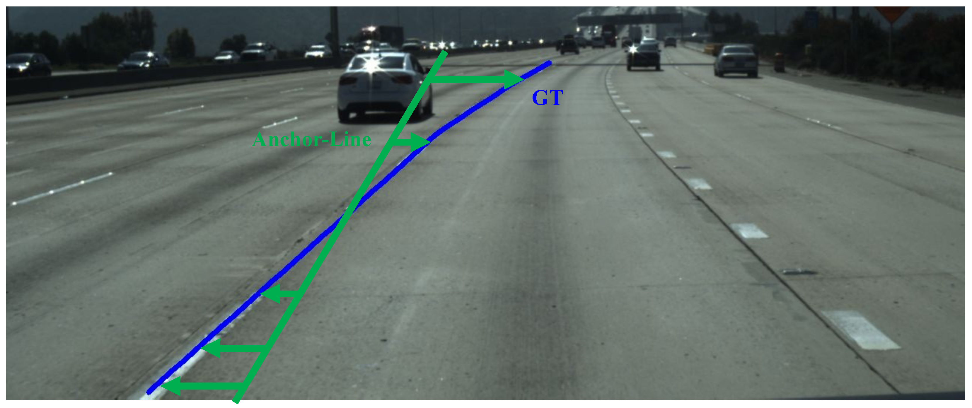
Therefore, this paper proposes a quality-guided lane line reference mechanism to optimize the lane line modeling process and achieve more flexible lane line representations. Inspired by the fine-grained object detection (FGOD) and the concept of computing relative offsets of reference points in Conditional DETR, this method addresses the poor adaptability of anchor lines to the complex shapes of lane lines by designing a two-stage regression reference, as shown in Figure 2. The proposed strategy enhances the flexibility of explicit regression references, enabling them to better adapt to the complex and diverse shapes of lane lines, thereby alleviating the issue where incorrectly sampled features from erroneous line anchors mislead lane detection [15,27]. In summary, this strategy aims to improve the adaptability of both explicit regression references and the dense feature sparsification method (i.e., line anchor sampling) with respect to flexible lane lines so as to better accommodate the complex shapes of lane lines.
Specifically, the process first initializes the reference starting point and the angle between the line extending from this starting point and the image edge, which is followed by predicting the x-direction offset of the sampling points on the line. Due to the visual magnification distortion present in onboard frontview images [5], the initial reference lines at curves may exhibit significant positional errors from ground truth coordinates. In such regions, the network requires more global information, while offset variations in other areas increase the network’s learning difficulty. To address this, this study introduces preset lane lines with predicted offsets as a second reference. This reference is entirely based on image features and is learnable, offering greater flexibility in the starting point, initial direction, and lane-fitting degree, making it more suitable for real-world scenarios. This reference generation strategy avoids confusion caused by insufficient visual information at the starting point due to poor occlusion, lighting conditions, etc. Additionally, lane lines in this paper are represented using equally spaced 2D sampled point sets to achieve lane line depiction.
l k = ( x k 1 , y k 1 ) , ( x k 2 , y k 2 ) , , ( x N k , y N k )
Here, k is the index of the lane. y k i depends on the image height, where k i is uniformly sampled from the i-th value of N in the y-direction, i.e., y k i = H N 1 × i .

3.3. Lane Pre-Selection Mechanism

To obtain sparse and high-quality regression references, which helps reduce the computational load of subsequent multi-scale feature fusion and lane line detection, thereby enabling high-precision lane line detection with a small number of features, this paper proposes a Lane Pre-selection Mechanism (LPsM) to achieve information aggregation and sparsity. This mechanism serves as the core component of the quality-guided lane line reference mechanism. Through the lane pre-screening mechanism, it provides sparse and high-quality features for the subsequent reference generation head.
Recent advancements in initial lane information collection algorithms, such as heat-map-based CondLaneNet [3] and ADNet [24], primarily follow a two-stage approach. However, these methods involve substantial redundant computations. Given that most forward-facing images depict four-lane scenarios at high resolution, with the processing width of each lane typically around 30 pixels [16], a large portion of the image does not contain lane information. This leads to bias in feature grids, highlighting the need for more efficient methods.
Moreover, after studying classical lane detection methods such as CondLantNet [3] and CLRNet [4], it was found that 256 channels are sufficient to store lane information; therefore, this study directly uses 1 × 1 convolution to perform feature aggregation in the channel dimension, reducing feature complexity. The reference generation head in this paper is similar to the classical object detection method FCOS, where one grid corresponds to one lane reference. This paper preprocesses this 256 channel feature grid to predict lane references. However, after 32× downsampling, the feature grid of the CULane dataset contains 10 × 25 grids, while there are only four to six lanes in this dataset, resulting in significant redundancy. Thus, sparsity processing is applied to these 250 grids, retaining 64 high-quality proposal grids. The specific method involves aggregating information within individual grids and performing information interaction between lane proposal features (LFAM2d, see Section 3.4) to calculate weights required for feature sparsification, drawing inspiration from classic concepts such as CBAM, SE, and residual connections. Additionally, this study uses wide range values to amplify weight differences, reducing the computational burden of the sparse layer. Subsequently, the filtered proposal features are used by the reference generation head to generate flexible lane references, which also serve as the basis for multi-scale, adaptive sparse lane feature sampling in the second stage.
The LPsM is designed to filter proposed features before prediction, as illustrated in Figure 3. Specifically, it first receives features from the backbone network with a 32× downsampling rate, which is input in the form of ( 512 , H 16 , W 16 ) . Then, a Stem layer composed of 1 × 1 convolutions aggregates these features into ( 256 , H 16 , W 16 ) . Subsequently, the lane feature attention mechanism proposed in Section 3.4 is employed to aggregate information from lane reference proposals and facilitate interaction among proposed features, resulting in high-quality, discriminative lane reference proposal features, with the output still maintaining the shape ( 256 , H 16 , W 16 ) . Finally, a linear layer ( H 16 × W 16 , N ) filters the lane reference proposal features to produce features of size ( 256 , N ) , where N represents the desired number of output lane references.

3.4. Lane Feature Attention Module

In autonomous driving scenarios, lane detection faces a dual contradiction between the need for global semantic correlation and local detailed features: on one hand, it requires establishing topological relationships that maintain the continuous orientation of lane themselves; on the other hand, it needs to preserve precise representations of the edges of near-field lane lines. To adaptively perform dense feature sparsification to accommodate the complex and diverse shapes of lane lines, redundant features in the feature map must be filtered out.
To address the above issues, this paper proposes a full-scale lane feature attention mechanism (LFAM). Its core design principles include (1) establishing a cross-scale feature interaction mechanism to enhance the representational capability of key information through feature aggregation and (2) introducing a feature competition mechanism to achieve the dynamic pruning of redundant features. This module adapts to different stage requirements through two forms. In the first stage, the LFAM operates on 2D feature grids with a shape of B , C , H , W and outputs proposal feature sets with a shape of B , C , N , where B denotes the batch size, C represents the amount of feature information per lane proposal, H and W are the height and width of the feature grid, respectively, and H × W corresponds to the number of lane proposals. In the second stage, it operates on multi-scale proposal features with a shape of B , 2 C , N to complete the adaptive multi-scale weighted fusion of proposal features, outputting fused proposal features with a shape of B , C , N .
It is important to note that besides differences in input feature shapes, the 2D and 1D forms of this module also differ in the purpose of enhancing features. In the first stage, it aims to sparsify the number of lanes to generate high-quality proposals. Inspired by the FCOS paradigm, each feature point corresponds to a proposal, which encapsulates information from each feature unit along the channel dimension and is associated with different lane lines in the spatial dimension. Given that the number of units in the feature grid downsampled by a factor of 16 far exceeds the number of real annotations, a selection process is necessary. This selection requires distinctiveness among features, so the primary role of the module in the first stage is to enhance the discriminative capability of features. In the second stage, instead of sparsifying lane features, the module sparsifies lane feature weights after calculating fusion weights, thereby achieving adaptive weighted feature fusion.
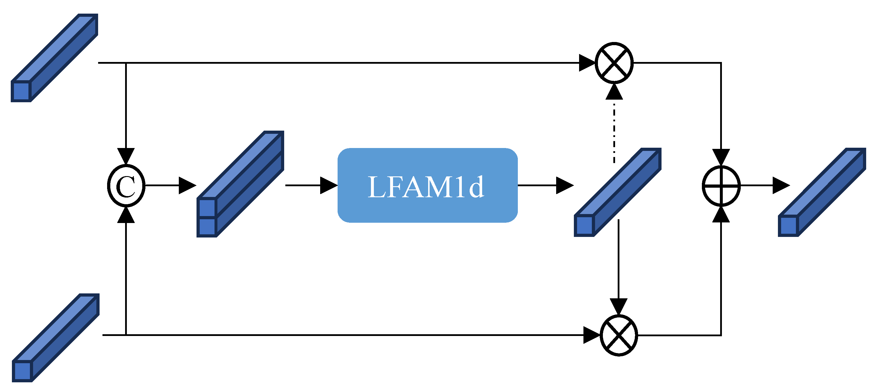
Specifically, as illustrated in Figure 4, the LFAM module fully considers the requirements for the full-scale interaction of lane features and sparsification, innovatively integrating feature aggregation and competition mechanisms. The specific implementation includes the following key components. (1) Lane Feature Information Aggregation: The lane feature global aggregation module is improved based on the MS-CAM from the AFF module proposed by Dai Yimian [28]. This study removes the sigmoid activation constraint in the original MS-CAM and directly uses wide range attention results as channel fusion weights, enabling the module to perform sparse feature operations. This facilitates channel aggregation, aggregating the lane’s existing features to enhance their integrity and global coherence. (2) Gaussian Competition Mechanism: Since comparisons between lane features occur during the screening or fusion processes, feature distinctiveness is required for subsequent networks to better differentiate lanes. To improve screening, a competition strategy based on probability distributions is proposed. For each lane feature f n R C , Gaussian parameters N μ n , σ n 2 are calculated, where μ n = E f n and σ n = V a r f n . The competition factor is defined as α n = Conv concat μ n , σ n . Through Gaussian distribution calculations, this mechanism differentiates lane features to suppress interference from low-quality features. (3) Residual Stabilization Connection: To prevent information loss during feature sparsification, a feature path residual mechanism is constructed: f ^ n = λ · f n α n + 1 λ · f n . Here, ⊗ denotes element-wise multiplication, and λ is a learnable balancing parameter.

3.5. Multi-Scale Proposal Feature Fusion

The successful application of dense feature sparsification technology has revealed that the number of features required for lane line detection is significantly smaller than the total number of features in the entire image [4,7,23,24]. Current mainstream methods generally follow technical solutions from the object detection field in feature enhancement and fusion processing; however, such dense computing methods are fundamentally contradictory to the sparse characteristics of lane line features. The full image feature-oriented computation paradigm not only leads to significant computational redundancy but also contradicts the real-time requirements of lane line detection tasks. Therefore, there is an urgent need to design a multi-scale feature fusion method tailored for lane line detection tasks to break through the limitations of existing technical solutions. Different from the Feature Pyramid Network (FPN) which employs element-wise operations, this module bypasses these operations and directly performs feature fusion on high-quality proposal features. This approach leverages the sparsity of lane features, thereby reducing unnecessary computational overhead. Furthermore, this study replaces the traditional 1:1 additive fusion operation with an adaptive weight operation, further enhancing the efficiency and specificity of the method proposed in this section. Benefiting from the high-quality lane line proposal features generated in the first section, this paper proposes Multi-scale Proposal Feature Fusion (MsPF), which directly performs feature enhancement and fusion on the proposal features, as shown in Figure 5. The structure of AWMF mainly consists of two parts: feature fusion (Conv 1d(k = 9), Self Attention) and feature fusion (AWMF). This module fully leverages the sparse distribution characteristics of lane lines, avoiding element-wise computations on densely distributed features across the entire image, thereby reducing redundant computations of lane line features. Additionally, this section replaces the 1:1 fusion operation in the pyramid network with adaptive weights.
This module is primarily divided into two components: lane information interaction and adaptive multi-scale information fusion of lane. Among them, the line information interaction part includes intra-lane information interaction and inter-line information interaction. The intra-lane information interaction employs a 1D Conv(k = 9) to realize information exchange between features of adjacent sampling points on lane, leveraging the local continuity of the lane to enhance lane features. The inter-line information interaction uses a linear focused attention module [29] to facilitate information interaction between features of different lanes, aiming to enhance features from a global perspective and compensate for information bias in sampled features. Subsequently, the adaptive multi-scale information fusion part is presented, named the Adaptive Weighted Fusion Module (AWMF, see Figure 6).
This subsection first concatenates and stores the results of intra-lane information interaction and inter-lane information interaction. Then, it uses the 1D form of the LFAM to calculate the weights of features and utilizes these weights to perform adaptive weighted multi-feature fusion on high-level and low-level features. The corresponding formula of this module is as follows:
F w e i g h t l = C S A M 1 d c o n c a t F g , F l , F w e i g h t g = 1 C S A M 1 d c o n c a t F g , F l , F f u s i o n = F g × F w e i g h t g + F l × F w e i g h t l .
Among them, F l and F g are the adaptive fusion weights of low-level and high-level features.

3.6. Label Assignment and Loss Function

3.6.1. Definition of Lane Distance

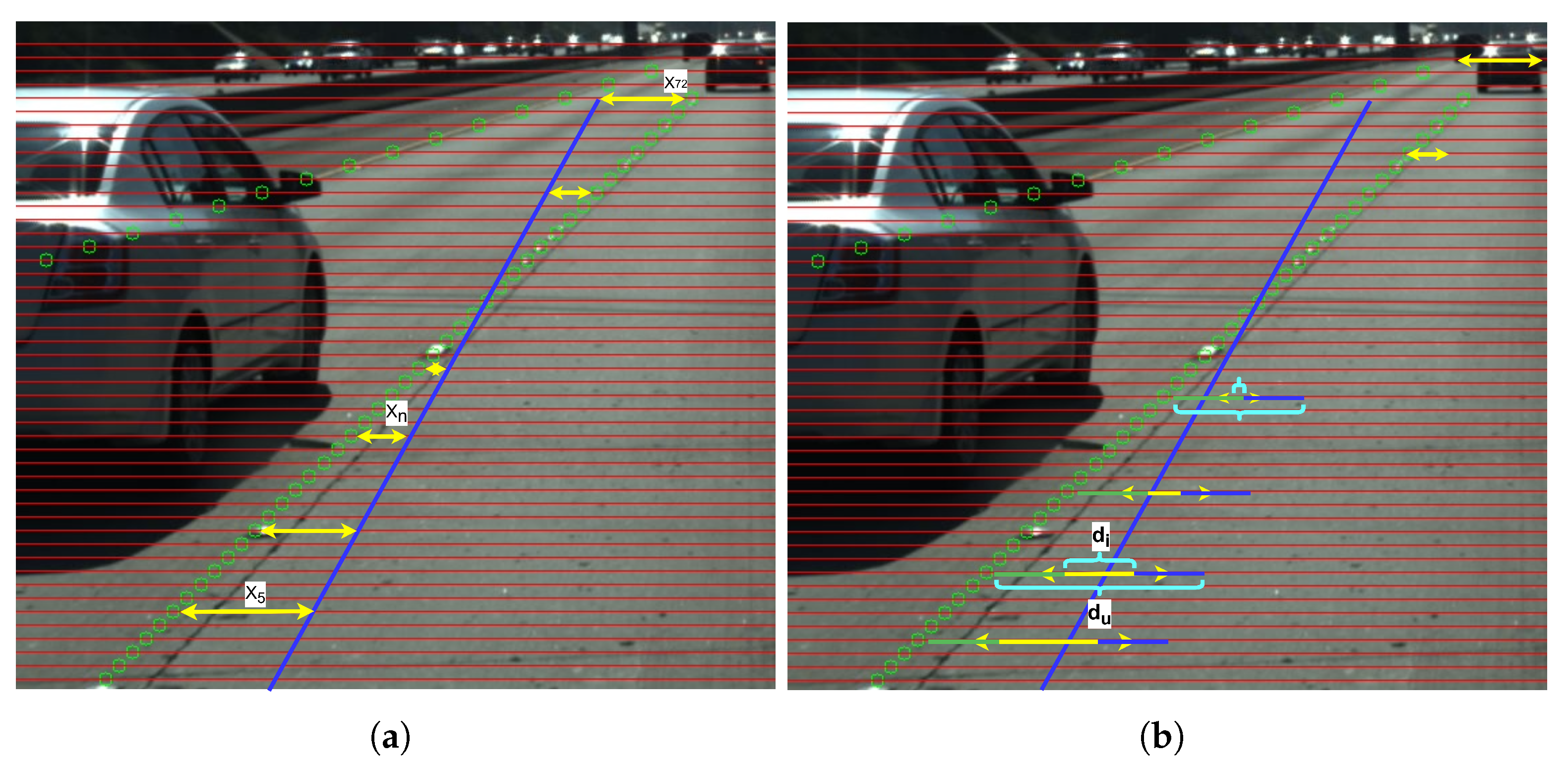
The definition of lane distance used in this subsection is adapted from the label storage format of the TuSimple dataset. For an image, equally spaced height sampling is performed at yi, where i ranges from 0 to 71. Across these 72 height levels, the x-direction offset between the predicted lanes and ground truth labels is used as the L1 distance metric to measure the distance between lanes, as shown in Figure 7a. To facilitate better network learning, the points of a lane at a specific height are expanded into line segments with a width r = 9. The endpoint coordinates of these segments at that height are defined as P = ( x i g r , x i g + r ) . By leveraging the concept of Jaccard similarity, the L1 distance between offsets is extended to the Jaccard distance for lanes, as illustrated in Figure 3 and Figure 7b.
Among them, the formula for the Jaccard distance of lanes at a certain height in Figure 7 is shown below:
J D = d i o d i u = min ( x i p + r , x i g + r ) max ( x i p r , x i g r ) max ( x i p + r , x i g + r ) min ( x i p r , x i g r )
Here, x i p + r and x i p r are expanded from the point x i p , while x i g + r and x i g r are the corresponding expanded points of the lane line’s points. Notably, d i o may take a negative value, indicating that the predicted lane line and the ground truth lane have no intersection, which allows optimizing non-overlapping scenarios. The value range of JD is 1 , 1 , representing the similarity between the predicted lane and the ground truth lane. A value of 1 indicates complete overlap, while a value less than or equal to 0 indicates a farther distance between the predicted lane line and the ground truth lane. With the defined lane distance, the loss function for lanes and the label matching cost can be designed.

3.6.2. Loss Function

Clearly, a higher Jaccard similarity of the lane indicates better prediction performance. Therefore, this paper defines 1 J D as the distance loss L J D for the lane, as shown in Equation (4):
L J D = 1 J D
if only L J D is used as the localization loss, theoretically, special cases may occur where the two ends of the lane are misaligned or the predicted lane intersects with the ground truth lane. To address this issue, the absolute value of the lane length, the loss related to the correspondence degree of the starting points, and the confidence loss are introduced, as shown in Equation (5):
L t o t a l = w c l s L c l s + w x y t l L x y t l + w L J D L L J D
where L cls is calculated using focal loss on the confidence of the predicted lane results; L xytl is the result of the L1 loss for the starting points of the predicted lane, the starting points of the ground truth lane, the average tilt angle of the lane, and the length of the lane represented by the number of occupied pixels. w cls , w xytl , and w LJD are weight parameters that can be adjusted according to actual conditions.

3.6.3. Label Assigner

The label-matching strategy in this section is consistent with CLRNet, adopting a matching approach similar to SimOTA. For each ground truth label, this method matches 1 to n predicted lanes, where n is determined by the confidence of the top n predicted lane—the higher the confidence, the more matches are made. The basis for matching is defined in Equation (6), which constructs a weighted sum of lane similarity and confidence:
C assign = w sim C sim + w cls C cls
Here, C cls represents the common focal cost used in object detection. C sim (see Equation (7)) is a metric that quantifies the similarity between the predicted and ground truth lane, comprising three components: the distance of starting points C dis , the angle difference C theta , and the sum of distances of lane sampling points C xy .
C sim = C dis · C xy · C theta 2

4. Experimental Settings

4.1. Datasets

4.1.1. CULane

CULane [16] is a large-scale, comprehensive, and challenging lane detection dataset, containing 133,235 frames of images, with 88,880 frames used for the training set, 9675 for the validation set, and 34,680 for the test set. The dataset covers scenarios such as urban areas and rural highways, where each image is annotated with up to four lanes, including occluded parts, while oncoming lanes are not annotated. The test set is divided into a normal category and eight challenging categories, including crowded traffic, nighttime scenes, blurred lane lines, the presence of shadows, the presence of lane markings, glare, curves, and intersections. Each frame is manually annotated using cubic spline curves. Each annotated image has a resolution of 1640 × 590 pixels. The dataset can be downloaded from https://xingangpan.github.io/projects/CULane.html (accessed on 24 September 2025).

4.1.2. TuSimple

The TuSimple [30] dataset was collected under good and moderate weather conditions on highways, involving road scenes at different times of day and varying traffic conditions. It consists of 6408 video clips captured from a viewpoint nearly aligned with the vehicle’s direction of travel, each containing 20 frames. Of these, 3268 clips are designated for the training set, 358 for validation, and 2782 for testing. Each video clip corresponds to a label file annotating lane line information from a monocular camera’s near-view perspective. Specifically, each image contains up to five lane lines, which are each represented by discrete 2D coordinate points along visible segments. The resolution of all annotated images is 1280 × 720 pixels. The dataset can be accessed via the provided link: https://github.com/TuSimple/tusimple-benchmark/issues/3 (accessed on 24 September 2025).

4.2. Evaluation Metrics

4.2.1. Area-Based Evaluation Metrics

The area-based evaluation metrics primarily use the Intersection over Union (IoU) between predicted lane lines and ground truth annotations as the measurement. When the IoU of the predicted lane lines (expanded to a 30-pixel width) and the ground truth annotations (similarly expanded) exceeds a predefined threshold τ , it is considered a true positive (TP) instance. Additionally, false positives (FPs) and false negatives (FNs) must be calculated, representing misdetections and missed detections, respectively. These three metrics are used to derive the test set evaluation metrics: precision, recall, and F1-score. Specifically, precision measures the proportion of true positives among all predicted positive instances, which is calculated as P r e c i s i o n = T P T P + F P ; recall measures the proportion of true positives among all actual positive instances, which is calculated as R e c a l l = T P T P + F N ; and the F1-score is the harmonic mean of precision and recall, which is calculated as F 1 = 2 × P r e c i s i o n × R e c a l l P r e c i s i o n + R e c a l l . These metrics ensure a balanced evaluation of both detection accuracy and completeness. In line with the official evaluation protocol, this study adopts the same evaluation protocol for the CULane dataset, where the IoU threshold ( τ ) is set to 0.5.

4.2.2. Distance-Based Evaluation Metrics

Based on the distance evaluation metrics considering spatial proximity criteria, the primary measurement focuses on the pixel distance between sampled points of predicted lane and ground-truth annotations at fixed heights. If the pixel distance between a sampled point on the predicted lane line and the corresponding point on the ground truth lane line at the same height is below a threshold τ , the sampled point is considered correct. Otherwise, it is classified as a false positive (FP) or false negative (FN). When the proportion of correct sampled points on a lane line exceeds a predefined threshold k, the lane is deemed accurately detected. Using these criteria, the evaluation metrics for the test set—accuracy (Acc), false positive rate (FP), and false negative rate (FN)—are calculated as follows: C c l i p denotes the number of correct sampled points on lane c, and S c l i p is the total number of sampled points on lane c. F P = F p r e d / N p r e d , where F p r e d is the number of incorrectly predicted lanes, and N p r e d is the total number of predicted lanes. F N = M p r e d / N g t where M p r e d is the number of missed ground truth lanes, and N g t is the total number of ground truth lanes. Consistent with official evaluation protocols, this study adopts the same metrics for the TuSimple datasets with a distance threshold τ = 20 pixels and a correctness threshold k = 0.85.

4.2.3. Model Inference Cost

Since lane detection tasks require a certain level of real-time performance, this study not only focuses on the accuracy of model localization but also our framework simultaneously optimizes the complexity of the model and its inference speed. We evaluate three key indicators: the number of parameters (Params), floating-point Operations (FLOPs), and frames per second (FPS). The parameter count represents the total trainable weights in the mode, which is mainly used to measure the size of the model (also known as spatial complexity). Floating-point operations refer to the total number of floating-point arithmetic operations required during model inference, which is primarily used to measure the computational complexity of the model (also known as time complexity). FPS indicates the throughput measured in images processed per second, which is mainly used to measure the inference speed of the model.

4.3. Implementation Details

The backbone network of this section utilizes ResNet [31] and DLA34 [32] pretrained on ImageNet [33]. All input data are resized to (800, 320). The data augmentation strategy aligns with [4,24], including horizontal flipping, random brightness and contrast adjustment, random HSV modulation, motion and median blurring, as well as random affine transformations (translation, rotation, and scaling). Experiments are configured with 64 proposals per image, where the feature dimension of each proposal depends on the sampled features—which are all set to 128. Each regression line is represented by 72 points, indicating the use of 36 sampled feature cells. Equidistant sampling is also adopted for curve modeling. For label assignment, top-k = 4. During inference, the F1-measure threshold is set to 0.5. Curve quality is measured using the Jaccard similarity coefficient along the horizontal axis at corresponding height points. Additionally, AdamW is employed as the optimizer with an initial learning rate of 0.0006 for 15 training epochs. The lane modeling, label assignment, and loss function implementations remain consistent with CLRNet to ensure fair comparisons. Code implementation is based on mmdetection [34] with data augmentation performed using the albumentations library. FPS and GFLOPs calculations are modified based on mmdetection’s code. To address the high sensitivity of hyperparameter tuning, we implement the EMA (Exponential Moving Average) to stabilize training to achieve accurate model convergence.

5. Results and Discussion

5.1. Visualization Comparison

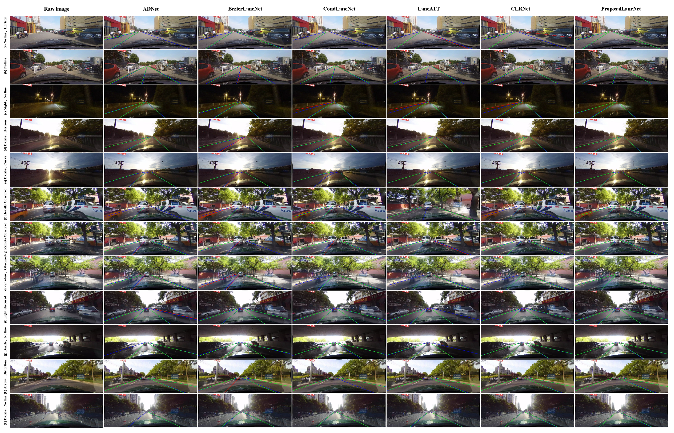
To more intuitively demonstrate the experimental effectiveness of the proposed method, this section conducts a comparative visual analysis with five classical methods, namely ADNet, BezierLaneNet, CondLaneNet, LaneATT, and CLRNet—across different scenarios, as shown in Figure 8.
First, ADNet and CondLaneNet exhibit varying degrees of detection errors, missed detections, or false detections when confronting challenging scenarios with different levels of occlusion (e.g., scenarios f, g, h, i, and j) where lane visual information is absent. This occurs because both methods rely on heat maps to detect lane starting points. However, they differ in their approaches: ADNet sets line anchors and samples features based on the detected starting point and overall lane angle, causing significant deviations when either the starting point or the angle is poorly estimated (e.g., in strong lighting conditions or curved scenarios such as e). In contrast, CondLaneNet mitigates sampling errors by incorporating conditional convolution for row classification, which is followed by predicting offsets relative to feature grid positions using the sampled features. Next, the BezierLaneNet method, when dealing with scenarios involving dashed lines (b), strong light (d), or varying levels of occlusion (f, g, h), shows minor positional deviations due to its reliance on single-scale features for detection, which lacks synergy between global and local information. For scenarios with nearly horizontal lanes (d) or curves (e), the method relies solely on the receptive field for detection, resulting in each feature grid containing minimal lane features due to its column-wise pooling for feature fusion. Additionally, when confronted with distorted central regions in monocular images or arrow markings (scenario k), BezierLaneNet’s flip fusion module constrained by its strong symmetry prior leads to false detections. LaneATT addresses these issues by using numerous line anchors for feature sampling and enabling an information interaction both within and between sampled features. However, its limitation lies in the strong prior of line anchors; when lane shapes or distributions deviate significantly from this prior (e.g., complex curves), severe positional misalignment occurs, leading to missed detections or minor positional errors. CLRNet combines the advantages of both ADNet and LaneATT, employing cross-attention for feature compensation. Although it adopts the concept of learnable anchors, they are only used for the starting point of the line anchor. Consequently, the linearity prior remains strong, causing inaccuracies when predicting curved lanes (e.g., scenario e). The ProposalLaneNet method proposed in this section utilizes high-quality lane priors as regression references and performs a comprehensive feature interaction between lane features and inter-lane features. This approach enables robust lane detection across all of the aforementioned complex scenarios.

5.2. Performance Comparison with Classical Methods

CULane: Table 1 shows the performance of algorithms on CULane in recent years. The algorithm proposed in this section not only achieves state-of-the-art (SOTA) levels among proposal-based methods but also remains the SOTA among all methods on this dataset. Specifically, the model using DLA-34 as the backbone outperforms the previous SOTA algorithm CLRNet by nearly 1 percentage point. Furthermore, all other models using different backbones also exceed the accuracy of CLRNet on the CULane dataset. Compared to the latest dense feature sparsification-based method ADNet (which is also a two-stage lane detection method), the model with ResNet18 as the backbone improves the F1-score from 77.56% to 80.09%, while the model with ResNet34 as the backbone improves accuracy from 78.94% to 80.52%. It is worth noting that the ProposalLaneNet results with the EMA (Exponential Moving Average) training strategy indicate that models trained without an EMA strategy can achieve better performance through parameter adjustment. The models proposed in this section use fewer parameters and have lower model complexity, even approaching minimalist models like BezierLaneNet. The ProposalLaneNet model based on ResNet-18 has only 9.88 GFLOPs and 13.14 million parameters. The ProposalLaneNet model based on DLA-34 also has only 16.27 GFLOPs and 17.20 million parameters, achieving the research goal of using fewer parameters to attain high accuracy.
TuSimple: Table 2 presents the test results of ProposalLaneNet and previous SOTA algorithms on the TuSimple test set. This dataset uses distance-based evaluation metrics, including F1-score, accuracy (Acc), false positives (FPs), and false negatives (FNs). The backbone network used is also noted. Through this table, it can be observed that the performance differences between various methods on this dataset are minimal. This is because the scenes in the dataset primarily consist of highway environments, which are relatively simple and homogeneous, and they are also commonly used as auxiliary test data to assess model robustness. The method proposed in this section achieves excellent results in the F1-score and false negative (FN) metrics, establishing a new SOTA with advantages of 0.50 and 0.56 percentage points, respectively. This breakthrough improvement demonstrates the effectiveness of the method proposed in this paper.

5.3. Ablation Study

5.3.1. Ablation Study of Core Modules

To validate the effectiveness of the method proposed in this section, this section features ablation experiments using DLA-34 as the primary backbone network, progressively adding components such as LPsM, MsPF, and AWFM. The baseline model for this paper is obtained by removing the components under verification. In the baseline model, the LPsM lacks the stem structure for information aggregation and any information enhancement mechanism; the prediction of the number of lane lines is directly obtained by filtering feature units through a convolutional layer. The reference model does not rely on image features but uses default reference lines from CLRNet. To more accurately validate the method’s effectiveness, 256 channels are used in the lane reference generation stage, consistent with the final model, outputting 64 lane lines. The experimental results of this section, as shown in Table 3, demonstrate that the proposed LPsM significantly improves model accuracy through feature aggregation. The F1-score increases from 74.70% to 78.92%, representing a substantial improvement. Subsequently, the MsPF is added. Note that the MsPF used here is a preliminary version. Since AWFM is part of MsPF, this experiment isolates it individually in this analysis to confirm the effectiveness of the progressive reference mechanism, which elevates the model’s F1-score to 80.23%. Finally, the AWFM module is added. This module considers the linear structure, interacts with information from points on the line, and achieves feature enhancement through inter-line information interaction. This approach ultimately improves the model’s accuracy to 81.02%, achieving state-of-the-art performance.

5.3.2. Ablation Study of the High-Quality Proposal Generation Head On

To generate sparse, high-quality proposals, ablation experiments based on core components reveal that the Lane Pre-selection Mechanism (LPsM) improves the F1-score from 74.70% to 78.92% compared to the baseline, demonstrating its effectiveness. Beyond the Lane Pre-selection Mechanism, the sparse high-quality proposal generation module includes a lane reference task head. As shown in Table 4, ablation experiments (a1–a8) were similarly conducted on this task head, where the feed-forward network uses fully connected features. The experiments investigate (1) whether classification and regression heads share fully connected features, (2) whether the task head uses a 1 × 1 convolutional layer or linear layer, and (3) the impact of including an auxiliary segmentation head. Experimental results indicate that the highest F1-scores consistently occur when using 1 × 1 convolutional layers. Without the auxiliary segmentation head, using decoupled features yields a higher F1-score, whereas with the auxiliary segmentation head, using shared features achieves a higher F1-score.

5.3.3. Ablation Study on the Efficacy of Multi-Scale Proposal Fusion

Similar to how generic semantic segmentation models cannot be directly and effectively transferred to lane detection tasks, existing methods use pyramid networks to provide the multi-scale information required for lane lines. While this module delivers high accuracy for lane detection, its whole image, pixel-level computations do not align with the sparse distribution characteristic of lane lines, introducing significant computational redundancy. The hierarchical features in Figure 1 originate directly from the hierarchical backbone network. The MsPF in this section adapts the concept of multi-scale fusion and applies it to the multi-scale proposal features derived from high-quality references, eliminating the need to compute all features. Specifically, the high-quality proposal features used in this section have dimensions 64 × 36 × C, whereas the features processed in the pyramid network are (20 × 50 + 40 × 100) × C, which is substantially larger. A comprehensive comparison between MsPF and FPN is provided in Table 5. In Table 5, the ADDF method replaces the Adaptive Weighted Fusion Module (AWMF) in MsPF with element-wise addition. The FPNX method introduces local and global information interaction into FPN. The MsPFX method first adjusts the FPN channel dimensions and then compares the results with ProposalLaneNet to ensure channel consistency.

5.3.4. Ablation Study on the Robustness of the Multi-Scale Proposal Fusion Method

To verify the role of multi-scale information provided by multi-scale proposals for the model, ablation experiments were conducted on another component designed to incorporate multi-scale information: the auxiliary segmentation head. As shown in Table 6, without MsPF, removing the auxiliary segmentation head causes the model’s F1-score to drop from 78.92% to 76.82%. This demonstrates that the auxiliary segmentation head plays a critical role in supplementing the model with multi-scale information. However, with the presence of multi-scale proposal features, removing the auxiliary segmentation head results in only a slight decrease of 0.18 percentage points in the F1-score. This sufficiently indicates that the multi-scale proposal fusion method offers greater robustness.

6. Conclusions

This paper fully incorporates the characteristics of lane lines—sparse distribution, elongated structure, and shape diversity—to propose ProposalLaneNet, which is a lane detection method featuring adaptive explicit references and sampling features. It primarily consists of the following aspects. (1) The Quality-Oriented Lane Reference (QOLR) generation strategy and the Multi-scale Proposal Feature fusion module (MsPF) address the poor adaptability of explicit references to complex shapes and the computational redundancy in feature processing, respectively. (2) The success of the MsPF is contingent on acquiring sparse, high-quality multi-scale proposal features. To achieve this, the Lane Pre-screening Mechanism (LPsM) was designed, preliminarily realizing the acquisition of such sparse, high-quality multi-scale proposal features. (3) The Lane Feature Attention Mechanism (LFAM) and the Adaptive Weighted Fusion Module (AWFM) are employed to achieve global–local information interaction at the lane level and adaptive multi-scale feature fusion, respectively, yielding robust lane detection results.
Ultimately, ProposalLaneNet achieves state-of-the-art (SOTA) performance on both the CULane and TuSimple datasets. Visualization analysis confirms that this method successfully mitigates issues prevalent in methods relying on explicit references and dense feature sparsification for detection.

Author Contributions

Conceptualization, W.Z. and B.C.; methodology, B.C.; software, L.T.; validation, L.T., D.L. and B.C.; formal analysis, L.T.; resources, D.L.; writing—original draft preparation, B.C.; writing—review and editing, W.Z. and L.T.; visualization, D.L.; funding acquisition, L.T. All authors have read and agreed to the published version of the manuscript.

Funding

Funding: The Project Supported by the Open Fund of Key Laboratory of Urban Land Resources Monitoring and Simulation, Ministry of Natural Resources (No. KF-2023-08-18).

Conflicts of Interest

The authors declare no conflicts of interest.

References

  1. Qin, Z.; Wang, H.; Li, X. Ultra Fast Structure-Aware Deep Lane Detection. In Proceedings of the European Conference on Computer Vision, Glasgow, UK, 23–28 August 2020; Vedaldi, A., Bischof, H., Brox, T., Frahm, J.M., Eds.; Springer: Berlin/Heidelberg, Germany, 2020; pp. 276–291. [Google Scholar] [CrossRef]
  2. Feng, Z.; Guo, S.; Tan, X.; Xu, K.; Wang, M.; Ma, L. Rethinking Efficient Lane Detection via Curve Modeling. In Proceedings of the 2022 IEEE/CVF Conference on Computer Vision and Pattern Recognition, New Orleans, LA, USA, 22–24 June 2022; pp. 17041–17049. [Google Scholar] [CrossRef]
  3. Liu, L.; Chen, X.; Zhu, S.; Tan, P. CondLaneNet: A Top-to-down Lane Detection Framework Based on Conditional Convolution. In Proceedings of the 2021 IEEE/CVF International Conference on Computer Vision, Montreal, QC, Canada, 11–17 October 2021; pp. 3753–3762. [Google Scholar] [CrossRef]
  4. Zheng, T.; Huang, Y.; Liu, Y.; Tang, W.; Yang, Z.; Cai, D.; He, X. CLRNet: Cross Layer Refinement Network for Lane Detection. In Proceedings of the 2022 IEEE/CVF Conference on Computer Vision and Pattern Recognition, New Orleans, LA, USA, 19–23 June 2022; pp. 888–897. [Google Scholar] [CrossRef]
  5. Qin, Z.; Zhang, P.; Li, X. Ultra Fast Deep Lane Detection With Hybrid Anchor Driven Ordinal Classification. IEEE Trans. Pattern Anal. Mach. Intell. 2024, 46, 2555–2568. [Google Scholar] [CrossRef] [PubMed]
  6. Su, J.; Chen, C.; Zhang, K.; Luo, J.; Wei, X.; Wei, X. Structure Guided Lane Detection. arXiv 2021, arXiv:2105.05403. [Google Scholar] [CrossRef]
  7. Tabelini, L.; Berriel, R.; Paixão, T.M.; Badue, C.; De Souza, A.F.; Oliveira-Santos, T. Keep your Eyes on the Lane: Real-time Attention-guided Lane Detection. In Proceedings of the IEEE/CVF Conference on Computer Vision and Pattern Recognition (CVPR), Virtual, 19–25 June 2021; pp. 294–302. [Google Scholar] [CrossRef]
  8. Tabelini, L.; Berriel, R.; Paixão, T.M.; Badue, C.; De Souza, A.F.; Oliveira-Santos, T. PolyLaneNet: Lane Estimation via Deep Polynomial Regression. In Proceedings of the 25th International Conference on Pattern Recognition (ICPR), Virtual, 10–15 January 2021; pp. 6150–6156. [Google Scholar] [CrossRef]
  9. Wang, J.; Ma, Y.; Huang, S.; Hui, T.; Wang, F.; Qian, C.; Zhang, T. A Keypoint-based Global Association Network for Lane Detection. In Proceedings of the 2022 IEEE/CVF Conference on Computer Vision and Pattern Recognition (CVPR), New Orleans, LA, USA, 21–24 June 2022; pp. 1382–1391. [Google Scholar] [CrossRef]
  10. Chen, H.; Wang, M.; Liu, Y. BSNet: Lane Detection via Draw B-spline Curves Nearby. arXiv 2023, arXiv:2301.06910. [Google Scholar] [CrossRef]
  11. Lin, T.Y.; Dollár, P.; Girshick, R.; He, K.; Hariharan, B.; Belongie, S. Feature Pyramid Networks for Object Detection. In Proceedings of the 2017 IEEE Conference on Computer Vision and Pattern Recognition, Honolulu, HI, USA, 21–26 July 2017; pp. 936–944. [Google Scholar] [CrossRef]
  12. Li, W.; Zhao, D.; Yuan, B.; Gao, Y.; Shi, Z. PETDet: Proposal Enhancement for Two-Stage Fine-Grained Object Detection. IEEE Trans. Geosci. Remote Sens. 2024, 62, 5602214. [Google Scholar] [CrossRef]
  13. Sun, P.; Zhang, R.; Jiang, Y.; Kong, T.; Xu, C.; Zhan, W.; Tomizuka, M.; Li, L.; Yuan, Z.; Wang, C.; et al. Sparse R-CNN: End-to-End Object Detection with Learnable Proposals. In Proceedings of the 2021 IEEE/CVF Conference on Computer Vision and Pattern Recognition, Virtual, 19–25 June 2021; pp. 14449–14458. [Google Scholar] [CrossRef]
  14. Cai, Z.; Vasconcelos, N. Cascade R-CNN: Delving Into High Quality Object Detection. In Proceedings of the 2018 IEEE/CVF Conference on Computer Vision and Pattern Recognition, Salt Lake City, UT, USA, 18–23 June 2018; pp. 6154–6162. [Google Scholar] [CrossRef]
  15. Meng, D.; Chen, X.; Fan, Z.; Zeng, G.; Li, H.; Yuan, Y.; Sun, L.; Wang, J. Conditional DETR for Fast Training Convergence. In Proceedings of the 2021 IEEE/CVF International Conference on Computer Vision, Montreal, BC, Canada, 11–17 October 2021; pp. 3631–3640. [Google Scholar] [CrossRef]
  16. Pan, X.; Shi, J.; Luo, P.; Wang, X.; Tang, X. Spatial as Deep: Spatial CNN for Traffic Scene Understanding. In Proceedings of the AAAI Conference on Artificial Intelligence, New Orleans, LA, USA, 2–7 February 2018. [Google Scholar] [CrossRef]
  17. Zheng, T.; Fang, H.; Zhang, Y.; Tang, W.; Yang, Z.; Liu, H.; Cai, D. RESA: Recurrent Feature-Shift Aggregator for Lane Detection. In Proceedings of the AAAI Conference on Artificial Intelligence, Virtual, 2–9 February 2021; Volume 35, pp. 3547–3554. [Google Scholar] [CrossRef]
  18. Wang, Z.; Ren, W.; Qiu, Q. LaneNet: Real-Time Lane Detection Networks for Autonomous Driving. arXiv 2018, arXiv:1807.01726. [Google Scholar]
  19. Abualsaud, H.; Liu, S.; Lu, D.B.; Situ, K.; Rangesh, A.; Trivedi, M.M. LaneAF: Robust Multi-Lane Detection with Affinity Fields. IEEE Robot. Autom. Lett. 2021, 6, 7477–7484. [Google Scholar] [CrossRef]
  20. Ko, Y.; Lee, Y.; Azam, S.; Munir, F.; Jeon, M.; Pedrycz, W. Key Points Estimation and Point Instance Segmentation Approach for Lane Detection. IEEE Trans. Intell. Transp. Syst. 2022, 23, 8949–8958. [Google Scholar] [CrossRef]
  21. Qu, Z.; Jin, H.; Zhou, Y.; Yang, Z.; Zhang, W. Focus on Local: Detecting Lane Marker from Bottom Up via Key Point. In Proceedings of the 2021 IEEE/CVF Conference on Computer Vision and Pattern Recognition, Virtual, 19–25 June 2021; pp. 14117–14125. [Google Scholar] [CrossRef]
  22. Liu, R.; Yuan, Z.; Liu, T.; Xiong, Z. End-to-end Lane Shape Prediction with Transformers. In Proceedings of the 2021 IEEE Winter Conference on Applications of Computer Vision, Virtual, 5–9 January 2021; pp. 3693–3701. [Google Scholar] [CrossRef]
  23. Li, X.; Li, J.; Hu, X.; Yang, J. Line-CNN: End-to-End Traffic Line Detection With Line Proposal Unit. IEEE Trans. Intell. Transp. Syst. 2020, 21, 248–258. [Google Scholar] [CrossRef]
  24. Xiao, L.; Li, X.; Yang, S.; Yang, W. ADNet: Lane Shape Prediction via Anchor Decomposition. In Proceedings of the 2023 IEEE/CVF International Conference on Computer Vision, Paris, France, 2–6 October 2023; pp. 6381–6390. [Google Scholar] [CrossRef]
  25. Jin, H.; Liao, S.; Shao, L. Pixel-in-Pixel Net: Towards Efficient Facial Landmark Detection in the Wild. Int. J. Comput. Vis. 2021, 129, 3174–3194. [Google Scholar] [CrossRef]
  26. Zhang, Y.; Zhu, L.; Feng, W.; Fu, H.; Wang, M.; Li, Q.; Li, C.; Wang, S. VIL-100: A New Dataset and A Baseline Model for Video Instance Lane Detection. In Proceedings of the 2021 IEEE/CVF International Conference on Computer Vision, Montreal, QC, Canada, 11–18 October 2021; pp. 15661–15670. [Google Scholar] [CrossRef]
  27. Liu, S.; Li, F.; Zhang, H.; Yang, X.; Qi, X.; Su, H.; Zhu, J.; Zhang, L. DAB-DETR: Dynamic Anchor Boxes are Better Queries for DETR. arXiv 2022, arXiv:2201.12329. [Google Scholar] [CrossRef]
  28. Dai, Y.; Gieseke, F.; Oehmcke, S.; Wu, Y.; Barnard, K. Attentional Feature Fusion. In Proceedings of the 2021 IEEE Winter Conference on Applications of Computer Vision, Virtual, 5–9 January 2021; pp. 3559–3568. [Google Scholar] [CrossRef]
  29. Han, D.; Pan, X.; Han, Y.; Song, S.; Huang, G. FLatten Transformer: Vision Transformer using Focused Linear Attention. In Proceedings of the 2023 IEEE/CVF International Conference on Computer Vision, Paris, France, 2–6 October 2023; pp. 5938–5948. [Google Scholar] [CrossRef]
  30. TuSimple TuSimple/Tusimple-Benchmark: TuSimple Competitions for CVPR2017. 2017. Available online: https://github.com/TuSimple/tusimple-benchmark (accessed on 24 September 2025).
  31. He, K.; Zhang, X.; Ren, S.; Sun, J. Deep Residual Learning for Image Recognition. In Proceedings of the 2016 IEEE Conference on Computer Vision and Pattern Recognition, Las Vegas, NV, USA, 27–30 June 2016; pp. 770–778. [Google Scholar] [CrossRef]
  32. Yu, F.; Wang, D.; Shelhamer, E.; Darrell, T. Deep Layer Aggregation. In Proceedings of the 2018 IEEE/CVF Conference on Computer Vision and Pattern Recognition, Salt Lake City, UT, USA, 18–23 June 2018; pp. 2403–2412. [Google Scholar] [CrossRef]
  33. Deng, J.; Dong, W.; Socher, R.; Li, L.J.; Li, K.; Fei-Fei, L. ImageNet: A large-scale hierarchical image database. In Proceedings of the 2009 IEEE Conference on Computer Vision and Pattern Recognition, Miami, FL, USA, 20–25 June 2009; pp. 248–255. [Google Scholar] [CrossRef]
  34. Chen, K.; Wang, J.; Pang, J.; Cao, Y.; Xiong, Y.; Li, X.; Sun, S.; Feng, W.; Liu, Z.; Xu, J.; et al. MMDetection: Open MMLab Detection Toolbox and Benchmark. arXiv 2019, arXiv:1906.07155. [Google Scholar] [CrossRef]
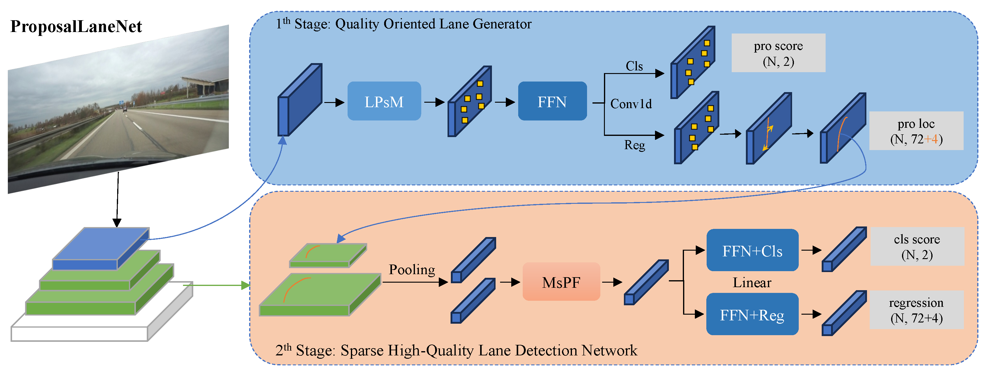
Figure 1. Overview of ProposalLaneNet. The network is divided into two stages: (1) generating sparse lane references via feature aggregation and pre-screening, and (2) performing multi-scale proposal feature fusion for efficient lane detection.
Applsci 15 10803 g001
Figure 2. Positional errors exist between traditional references and GT. Green serves as the basis for feature sampling, relying on the sampled features to predict offset quantities.
Applsci 15 10803 g002
Figure 3. Structure of the Lane Pre-selection Mechanism (LPsM). It compresses and refines backbone features through channel aggregation and attention; then, it selects sparse high-quality lane references.
Applsci 15 10803 g003
Figure 4. Structure of the 2D Lane Feature Attention Module (LFAM2d). The module performs feature enhancement and sparsification through three key components: global feature aggregation (using GAP and PRP units), Gaussian competition mechanism, and residual connections.
Applsci 15 10803 g004
Figure 5. Structure of the MsPF module, consisting of two core components: feature enhancement and adaptive weighted fusion, enabling multidimensional feature fusion.
Applsci 15 10803 g005
Figure 6. Structure of the AWMF module, demonstrating the adaptive weight fusion mechanism for multi-scale features.
Applsci 15 10803 g006
Figure 7. This is a schematic diagram defining lane distances. The diagram consists of two subfigures: (a) the L1 distance of lane lines; (b) the Jaccard distance of lane lines. The figure illustrates sampling points of lane lines at different heights and their corresponding distance calculation methods.
Applsci 15 10803 g007
Figure 8. Visual comparison of different lane detection methods under various challenging scenarios.
Applsci 15 10803 g008
Table 1. Results on the test set of CULane.
Method BackboneGFLOPs ↓FPS ↑GPU (TFLOPS)Eff.Total (%) ↑Normal (%) ↑Crowd (%)↑Dazzle (%) ↑Shadow (%) ↑No Line (%) ↑Arrow (%) ↑Curve (%)↑Cross (%) ↓Night (%) ↑
Traditional Lane Segmentation
SCNN [16](Ref. AAAI2018)VGG16328.47.55.11.4771.6090.6069.7058.5066.9043.4084.1064.40199066.10
RESA [17](Ref. AAAI2021)ResNet-3441.045.513.453.3974.5091.9072.4066.5072.0046.3088.1068.60189669.80
RESA [17](Ref. AAAI2021)ResNet-5043.035.713.452.6575.3092.1073.1069.2072.8047.7088.3070.30150369.90
Instance & Grid Lane Segmentation
UFLD [1](Ref. ECCV2020)ResNet-188.432310.630.4768.4087.7066.0058.4062.8040.2081.0057.90174362.10
UFLD [1](Ref. ECCV2020)ResNet-3416.917510.616.5172.3090.7070.2059.5069.3044.4085.7069.50203766.70
LaneAF [19](Ref. LRA2021)ERFNet22.22410.62.2675.6391.1073.3269.7175.8150.6286.8665.02184470.90
LaneAF [19](Ref. LRA2021)DLA-3423.62010.61.8977.4191.8075.6171.7879.1251.3886.8872.70136073.03
CondLaneNet [3](Ref. ICCV2021)ResNet-1810.222010.121.7878.1492.8775.7970.7280.0152.3989.3772.40136473.23
CondLaneNet [3](Ref. ICCV2021)ResNet-3419.615210.115.0578.7493.3877.1471.1779.9351.8589.8973.88138773.92
CondLaneNet [3](Ref. ICCV2021)ResNet-10144.85810.15.7479.4893.4777.4470.9380.9154.1390.1675.21120174.80
UFLDv2 [5](Ref. TPAMI2022)ResNet-18-33035.69.2774.791.773.064.674.747.287.668.7199870.2
UFLDv2 [5](Ref. TPAMI2022)ResNet-34-16535.64.6375.992.574.965.775.349.088.570.2186470.6
Keypoint-Based Lane Detection
FOLOLane [21](Ref. CVPR2021)ERFNet-4014.02.8678.8092.7077.8075.2079.3052.1089.0069.40156974.50
GANet-S [9](Ref. CVPR2022)ResNet-1821.27 *15314.010.9378.7993.2477.1671.2477.8853.5989.6275.92124072.75
GANet-M [9](Ref. CVPR2022)ResNet-3430.72 *12714.09.0779.3993.7377.9271.6479.4952.6390.3776.32136873.67
GANet-L [9](Ref. CVPR2022)ResNet-10189.45 *6314.04.5079.6393.6778.6671.8278.3253.3889.8677.37135273.85
Curve-Based Lane Detection
BézierLaneNet [2](Ref. CVPR2022)ResNet-187.5 *21313.415.9073.6790.2271.5562.4970.9145.3084.0958.9899668.70
BézierLaneNet [2](Ref. CVPR2022)ResNet-3415.82 *15013.411.1975.5791.5973.2069.2076.7448.0587.1662.4588869.90
BSNet [10](Ref. ARXIV2023)ResNet-18-19710.618.5879.6493.4677.9374.2581.9554.2490.0573.62140075.11
BSNet [10](Ref. ARXIV2023)ResNet-34-13310.612.5579.8993.7578.0176.6579.5554.6990.7273.99144575.28
BSNet [10](Ref. ARXIV2023)ResNet-101-4810.64.5380.0093.7578.4474.0781.5154.8390.4874.01125575.12
BSNet [10](Ref. ARXIV2023)DLA-34-11910.611.2380.2893.8778.9275.0282.5254.8490.7374.71148575.59
Proposal-Based Lane Detection
LaneATT [7](Ref. CVPR2021)ResNet-189.325013.418.6675.1391.1772.7165.8268.0349.1387.8263.75102068.58
LaneATT [7](Ref. CVPR2021)ResNet-3418.017113.412.7676.6892.1475.0366.4778.1549.3988.3867.72133070.72
LaneATT [7](Ref. CVPR2021)ResNet-12270.52613.41.9477.0291.7476.1669.4776.3150.4686.2964.05126470.81
CLRNet [4](Ref. CVPR2022)ResNet-1811.9102 *7.7613.1479.5893.3078.3373.7179.6653.1490.2571.56132175.11
CLRNet [4](Ref. CVPR2022)ResNet-3421.568 *7.768.7679.7393.4978.0674.5779.9254.0190.5972.77121675.02
CLRNet [4](Ref. CVPR2022)ResNet-10142.94610.64.3480.1393.8578.7872.4982.3354.5089.7975.57126275.51
CLRNet [4](Ref. CVPR2022)DLA-3418.566 *7.768.5180.4793.7379.5975.3082.5154.5890.6274.13115575.37
ADNet [24](Ref. ICCV2023)ResNet-18-8735.62.4477.5691.9275.8169.3976.2151.7587.7168.84113372.33
ADNet [24](Ref. ICCV2023)ResNet-34-7735.62.1678.9492.9077.4571.7179.1152.8989.9070.64149974.78
ProposalLaneNet ResNet-189.88 *135 *7.7617.4080.0993.5078.6672.7679.7653.0190.4071.7781875.49
ProposalLaneNet ResNet-3419.33 *93 *7.7611.9880.5293.7778.8473.5384.1254.1990.7972.71105475.83
ProposalLaneNet DLA-3416.27 *83 *7.7610.7081.0293.9079.9275.3283.8555.4790.2474.2796476.24
ProposalLaneNet DLA-34 ( e m a ) 16.27 *83 *7.7610.7081.3594.1480.4876.7584.4657.5190.7076.15133576.69
denotes the test results of this study, while all other results were sourced from the respective papers. ↑ indicates higher is better, ↓ indicates lower is better. GPU abbreviations: Titan Black (5.1 TFLOPS), 2080Ti (13.45 TFLOPS), 1080Ti (10.6 TFLOPS), 3090 (35.58 TFLOPS), T4 (7.76 TFLOPS), V100 (14.03 TFLOPS). Eff. represents the ratio of FPS to the theoretical FP32 performance (TFLOPS) of the GPU with higher values indicating greater efficiency.
Table 2. Results on the test set of TuSimple.
MethodBackboneF1-Measure ↑Accuracy ↑False Positives ↓False Negatives ↓
RESAResNet3496.9396.823.632.48
PolyLaneNetEfficientNetB090.6293.369.429.33
E2EERFNet96.2596.023.214.28
UFLDResNet3488.0295.8618.913.75
UFLDv2ResNet3496.2295.563.184.37
SGNetResNet34-95.87--
LaneATTResNet3496.7795.633.532.92
CondLaneNetResNet10197.2496.542.013.50
FOLOLaneERFNet96.5996.924.472.28
ADNetResNet1896.9096.232.913.29
ProposalLaneNetResNet1897.7496.342.821.72
Table 3. Overall ablation study of ProposalLaneNet-DLA34 on CULane.
BaselineLPsMMsPFAWFMF1-Measure (%)
74.70
78.92
80.23
81.02
Table 4. Ablation study of the high-quality proposal generation head on CULane.
StudyShared FeaturesDecoupled Features 1 × 1 Conv StacksLinear LayersAuxiliary SegmentationF1-Measure
a 1 76.15
a 2 76.78
a 3 77.73
a 4 77.19
a 5 78.92
a 6 78.27
a 7 77.82
a 8 78.52
Table 5. Comparison of MsPF and FPN.
MethodF1@50 (%)Flops (GFLOPs)Params (M)Input-Size
ADDF79.4815.8615.72(320, 800)
FPNX79.5917.818.22(320, 800)
MsPFX80.7515.8615.74(320, 800)
Table 6. Ablation of auxiliary segmentation.
Baseline + LsPMw.o.segF1 (%)
78.92
76.82
ProposalLaneNetw.o.segF1 (%)
81.02
80.98
Disclaimer/Publisher’s Note: The statements, opinions and data contained in all publications are solely those of the individual author(s) and contributor(s) and not of MDPI and/or the editor(s). MDPI and/or the editor(s) disclaim responsibility for any injury to people or property resulting from any ideas, methods, instructions or products referred to in the content.