Multi-Fidelity Neural Network-Aided Multi-Objective Optimization Framework for Shell Structure Dynamic Analysis

Featured Application

The results show that reliable surrogate quality is the key driver of optimization success. Multi-fidelity learning combined with curriculum strategies lowers simulation costs while directly improving Pareto-front solutions. This makes the approach attractive for industrial design tasks—such as civil engineering, aerospace, automotive, or energy components—where faster iterations and reduced computational budgets are essential, without sacrificing engineering reliability.

Abstract

We address surrogate-assisted multi-objective optimization for computationally expensive structural designs. The testbed is an axisymmetric laminated composite shell whose geometry, ply angles, and plywise materials are optimized to simultaneously (i) maximize separation of selected natural frequencies from a known excitation and (ii) minimize material cost. To reduce high-fidelity (HF) finite element evaluations, we develop a deep neural network surrogate framework with three variants: an HF-only baseline; a multi-fidelity (MF) pipeline using an auxiliary refinement network to convert abundant low-fidelity (LF) data into pseudo-HF labels for a single-fidelity evaluator; and a cascaded ensemble that emulates HF responses and then maps them to pseudo-experimental targets. During optimization, only surrogates are queried—no FEM calls—while final designs are verified by FEM. Pareto-front quality is quantified primarily by a normalized relative hypervolume indicator computed against an envelope approximation of the True Pareto Front, complemented where appropriate by standard indicators. A controlled training protocol and common validation regime isolate the effect of fidelity strategy from architectural choices. Results show that MF variants markedly reduce HF data requirements and improve Pareto-front quality over the HF-only baseline, offering a practical route to scalable, accurate design under strict computational budgets.

1. Introduction

Surrogate models are employed to reduce the number of high-fidelity evaluations by providing fast, learnable approximations of objectives and constraints—an especially valuable property in multi-objective evolutionary settings where populations of candidate designs must be evaluated in each generation. Consequently, the effectiveness of multi-objective optimization for engineering problems with computationally expensive objective function evaluations (e.g., finite element analyses) depends critically on the quality of the surrogate coupled with the optimization method (here: genetic algorithms) [1,2,3,4]. Within surrogate-assisted evolutionary computation, classical metamodeling frameworks (Kriging/co-Kriging, radial basis functions, polynomial response surfaces) and modern deep neural networks are used to approximate expensive simulators, balance bias–variance, and expose uncertainty information that can guide exploration [5,6,7,8]. In structural applications [9], such surrogates have supported composite-structure design, stacking-sequence optimization, and reliability-driven assessments under stringent computational budgets [10,11,12].

Deep neural networks have emerged as a versatile class of surrogate models, capable of representing highly nonlinear mappings between mixed discrete–continuous design variables and structural responses. Unlike classical metamodels, deep networks can scale to high-dimensional inputs, naturally incorporate categorical encodings, and learn hierarchical features that capture interactions among ply orientations, material choices, and geometric descriptors. Their flexibility has been demonstrated across a wide range of engineering applications, from structural dynamics to aerodynamic design, where they often outperform simpler regressors once sufficient training data become available [10,13,14].

In the context of multi-fidelity workflows, neural surrogates provide additional advantages. Architectures such as transfer-learning stacks, linear–nonlinear decompositions, or hybrid ensembles can exploit correlations between low- and high-fidelity models while remaining computationally efficient at inference [15,16,17,18,19]. Moreover, robust loss functions (e.g., MAE, arcsinh) and regularization techniques (dropout, batch normalization) help stabilize training with noisy or limited HF data improving generalization near the Pareto front where accuracy is most critical. These properties make deep networks a natural backbone for the present study, complementing classical surrogates such as Kriging/co-Kriging [4,20].

Recent advances have shown the importance of multi-fidelity strategies, where the fusion of low-fidelity (LF) and high-fidelity (HF) models can significantly reduce computational costs without compromising accuracy [15,16,21,22,23]. MF approaches leverage the strengths of both low-fidelity models, which are computationally inexpensive but less accurate, and high-fidelity models, which provide more precise results but require significantly more computational resources. These hybrid approaches have been successfully applied in various fields, from aerodynamic shape optimization [15,16,24] to fatigue analysis of welded joints [21], as well as in the optimization of laminated composite structures [22,23].

Beyond single-fidelity modeling, multi-fidelity strategies fuse inexpensive low-fidelity (LF) information with limited high-fidelity (HF) data to improve predictive accuracy at reduced cost. Established MF constructions include autoregressive/co-Kriging corrections, hierarchical regressors, and physics-aware mappings; analyses clarify when each is advantageous with respect to discrepancy structure, noise, and sample allocation [20,25]. In the deep-learning regime, MF surrogates leverage cross-fidelity correlations via stacked or transfer-learning architectures and discrepancy learning: demonstrations span aerodynamic shape optimization with MF deep neural networks, MF convolutional surrogates adapted by transfer learning, composite neural networks with online adaptive bases, and MF regression for parameter-dependent outputs; related MF stacks have also been validated in high-frequency antenna modeling [15,16,17,18,19]. For structural and fatigue analysis, MF surrogate-assisted workflows have been shown to accelerate welded-joint life assessments while preserving prediction quality [21].

Multi-fidelity strategies have also been used successfully in the optimization of dynamic properties of laminated composite structures. For instance, studies on composite shell structures have demonstrated the use of MF surrogate models to improve natural frequency prediction, vibration analysis, and buckling resistance, all while minimizing computational time [23,26]. This makes MF methods a strong candidate for optimizing laminated composites, which are widely used in aerospace and automotive industries due to their excellent strength-to-weight ratios and tailorability.

From a workflow perspective, we view surrogate construction as an iterative, data-centric loop. Initial designs are used to train a baseline surrogate; accuracy is then improved by targeted enrichment in regions with high contribution to the Pareto set or large posterior uncertainty. Curriculum learning (CL) offers a practical scheduling principle: training progresses from easier, coarse-resolution tasks to harder, high-accuracy ones, which stabilizes optimization-relevant generalization and reduces the budget of HF queries [27]. In practice, CL organizes training as a sequence that begins with simpler, lower-resolution problems and gradually advances to more complex, higher-resolution tasks. This method helps stabilize the generalization of optimization models and reduces the number of high-fidelity evaluations required during the optimization process. By focusing first on low-fidelity data, CL accelerates the surrogate model’s development and optimizes computational costs [28,29]. Empirical evidence from process systems shows that progressive/curriculum schemes can increase surrogate accuracy and training efficiency, a behavior we exploit by interleaving LF-dominated stages with HF-focused refinements [30]. In parallel, uncertainty-aware selection—available in both Kriging-type and neural network-based surrogates—prioritizes acquisitions that either reduce model uncertainty near the incumbent Pareto front or correct systematic discrepancies highlighted by MF mappings [4].

In applications where high-fidelity data are scarce or expensive, curriculum learning and multi-fidelity approaches can be combined to optimize the use of both types of data. In the design of laminated composite shells, for example, curriculum learning has been shown to improve surrogate model performance by first focusing on lower-fidelity data and then progressively incorporating higher-fidelity samples as the optimization progresses [28,31]. This approach significantly reduces the computational cost while ensuring that the surrogate model can effectively capture the complex relationships within the design space.

We select laminated composite structures as the running application because they combine exceptionally high stiffness-to-weight ratios and strength with fine-grained tailorability through stacking sequence and fiber orientation; at the same time, their dynamic behavior (e.g., natural frequencies, mode shapes, damping) is highly sensitive to layup decisions, boundary conditions, and manufacturing tolerances, which necessitates continual characterization and re-analysis across the design space [32,33]. The presence of discrete and continuous design variables (ply angles, counts, thicknesses), tight performance margins, and competing objectives (mass, stiffness, buckling resistance, dynamic response, cost) further amplifies the need for sample-efficient optimization. Variable-stiffness laminates expand this landscape and enable performance gains but introduce additional nonconvexity and modeling burden—making the case for surrogate and multi-fidelity modeling particularly strong [34]. Empirically, the literature documents a steady stream of dynamics-focused optimization studies (e.g., maximizing fundamental frequency or controlling vibrational response) that require repeated, costly analyses—precisely the regime where surrogate-assisted, multi-fidelity evolutionary search can deliver large savings without sacrificing accuracy [22,23,26].

Our study therefore examines surrogate definitions spanning single- and multi-fidelity neural networks, and analyzes how their predictive quality translates to optimization quality when coupled with the Non-dominated Sorting Genetic Algorithm II (NSGA-II) [3]. Optimization accuracy is quantified using Pareto-front quality indicators with respect to the true objectives, primarily hypervolume and relative hypervolume loss [35,36]. Beyond final-front metrics, we also consider computational efficiency (costly-evaluation savings), robustness across random seeds, and ablation studies that isolate the impact of MF fusion, CL scheduling, and uncertainty-aware enrichment. Together, these elements yield a principled, scalable recipe for surrogate-assisted multi-objective genetic optimization in high-fidelity engineering design.

2. Materials and Methods

2.1. The Structure

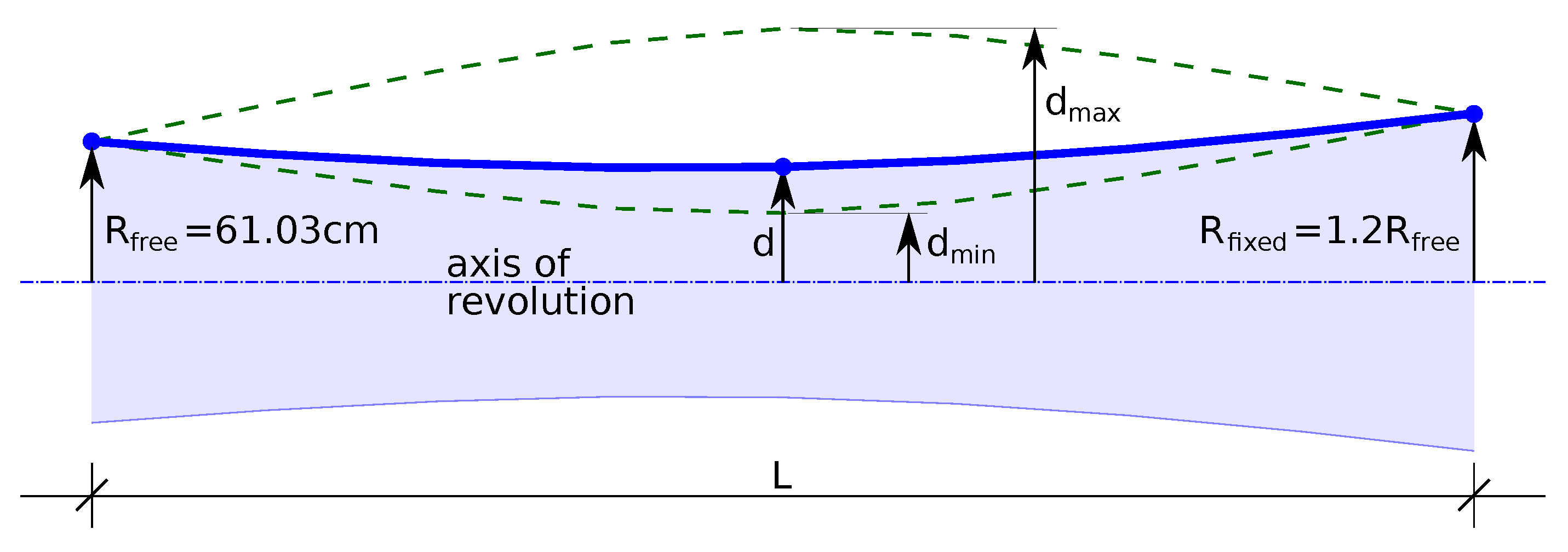
The finite element model adopts an axisymmetric layered-shell formulation: a two-dimensional meridional profile (Figure 1) is revolved to form a shell of revolution, and the laminate response is computed using classical lamination theory [32]. The reference geometry is a hyperboloid of revolution whose mid-surface is controlled by a single scalar “depth’’ parameter d, $30\mathrm{cm}\le d\le 110\mathrm{cm}$, that modulates the curvature reversal at the waist, permitting both convex and concave variants within one family (Figure 2); d is treated as a continuous design variable during optimization. The constant geometric parameters are fixed as $L=6$ m, $R_{\mathrm{free}}=61.03$ cm, and $R_{\mathrm{fixed}}=1.2R_{\mathrm{free}}$. The boundary conditions are the edge at $R_{\mathrm{fixed}}$ is fully clamped (all displacements constrained), while the opposite edge at $R_{\mathrm{free}}$ is free.

Competing cylindrical (Figure 2c) and conical baselines were examined at an earlier stage; here, we focus on the hyperboloidal profile due to its richer curvature control and the resulting flexibility in shaping global and local stiffness.

The shell has constant total thickness $t=1.6$ cm with a fixed eight-ply layup, with each ply of thickness $t/8$. The stacking sequence is denoted as $[{\lambda }_1/{\lambda }_2/\cdots /{\lambda }_8]$, where each ply angle ${\lambda }_i$ is discretized in $5^{\circ }$ steps over $[-{90}^{\circ },{90}^{\circ }]$ and treated as a decision variable. Material assignment is optimized at the ply level: for each lamina i, a categorical variable ${\mu }_i\in \{\mathrm{CFRP},\mathrm{GFRP},\mathrm{tFRP}\}$ selects either one of two fiber-reinforced composites (CFRP, GFRP) or a theoretical tFRP defined by property values averaged from CFRP and GFRP. A summary of the adopted properties is given in

Table 1. Properties of the three fiber-reinforced composites: CFRP, GFRP, and tFRP (cf. [37]).

Material	$\mathit{\mu }$	${\mathit{E}}_{\mathit{a}}$	${\mathit{E}}_{\mathit{b}}$	${\mathit{E}}_{\mathit{c}}$	${\mathit{\nu }}_{\mathit{ab}}$	${\mathit{\nu }}_{\mathit{ac}}$	${\mathit{\nu }}_{\mathit{bc}}$	${\mathit{G}}_{\mathit{ab}}$	${\mathit{G}}_{\mathit{ac}}$	${\mathit{G}}_{\mathit{bc}}$	Density $\mathit{\rho }$	Cost ${\mathit{c}}_{\mathit{\mu }}$
Label	[-]	[GPa]	[GPa]	[GPa]	[-]	[-]	[-]	[GPa]	[GPa]	[GPa]	[$\mathrm{kg}/{\mathrm{m}}^{\mathbf{3}}$]	[-]
CFRP	1	120	8	8	0.014	0.028	0.028	5	5	3	1536	10.20
tFRP	2	80	6	6	0.020	0.036	0.036	4	4	3	1428	5.78
GFRP	3	40	4	4	0.026	0.044	0.028	3	3	3	1320	1.36

(cf. [37]).

The resulting 17-component design vector

$$\mathbf{p}=\{{\lambda }_1,\dots ,{\lambda }_8,{\mu }_1,\dots ,{\mu }_8,d\}$$

(1)

combines one geometric parameter with eight angle variables and eight material choices. In the analysis, each lamina inherits orthotropic properties according to ${\mu }_i$, and the model captures the stiffness trade-offs among mass, strength, and cost while remaining compact enough for surrogate-assisted multi-objective optimization.

The selection of design variables and simulation models applied in this study follows from our earlier systematic analyses. In particular, lamination angles were adopted as primary variables since they have the strongest impact on stiffness and dynamic properties; in earlier works, they were treated as continuous variables, but it was shown that discretizations finer than $5^{\circ }$ increase computational complexity without providing noticeable improvements [38]. Similarly, different numbers of layers were examined (from 4 to 32), and it was demonstrated that increasing the number beyond 8–16 does not improve the optimized objective functions, while it substantially enlarges the design space [38]. Therefore, in the present work, eight layers and a $5^{\circ }$ step were chosen as rational compromises between accuracy and efficiency. The introduction of the geometric parameter d and material selection (CFRP, GFRP, tFRP) in [31] was an intentional step to test the proposed procedure in more complex optimization tasks, including geometry and cost optimization, and to study their influence on objectives such as frequency band width and material cost.

2.2. Finite Element Model

Two finite element discretizations are employed that differ solely in target mesh density. In both cases, the structure is modeled with four-node MITC4 multilayer shell elements consistent with first-order shear-deformation kinematics [39]. The nominal finite-element size (maximum edge length of an approximately square element) is denoted by h. For the reference, high-fidelity model $\mathcal{M}1$ we take $h\approx 1.25$ cm, acknowledging small spatial variations along the circumferential and meridional directions. A coarser companion model, $\mathcal{M}$5, is built with $h=5$ cm.

The finite element simulations were performed using the commercial software ADINA 9.8 [39]. All analyses were carried out in the implicit eigenvalue setting (modal analysis). The high-fidelity model $\mathcal{M}1$ employed a $600\times 400$ mesh, resulting in approximately 1,202,000 degrees of freedom, and required on average 888.36 s of CPU time per run. The $\mathcal{M}5$ model used a $120\times 80$ mesh with 48,400 degrees of freedom and an average CPU time of 59.02 s. Wall-clock times were not reported because they were not representative under varying thread availability and system load conditions. All computations were executed on a workstation equipped with an AMD EPYC^TM 7443P processor (24 CPU cores, base clock 2.85 GHz, maximum boost clock 4.0 GHz) and 256 GB of RAM.

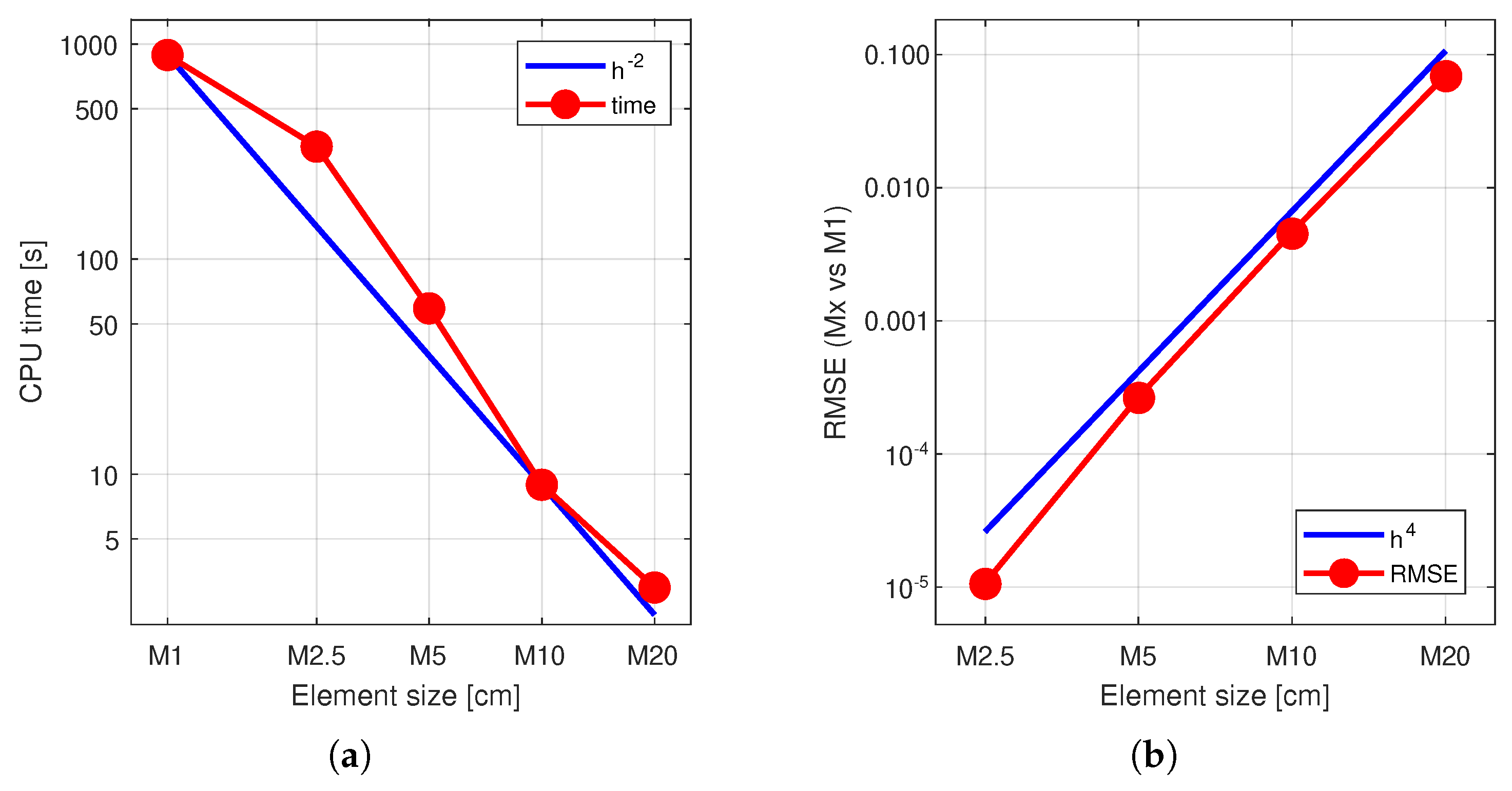
The two levels serve distinct purposes. $\mathcal{M}1$ provides the high-fidelity baseline used both for validation and for generating a pseudo-experimental target, whereas $\mathcal{M}$5 supplies inexpensive additional samples to enlarge the training corpus of the surrogate. Because $\mathcal{M}$5 elements are four times larger, the 2D mesh cardinality drops approximately by a factor of $4^2$, yielding a commensurate reduction in solution time (see Figure 3a). This comes at the cost of accuracy: in our setting, eigenfrequency errors grow on the order of $4^4$ when moving from $\mathcal{M}1$ to $\mathcal{M}$5 (see Figure 3b), a degradation explicitly handled by the downstream learning and optimization steps [28].

To emulate laboratory measurements and modeling discrepancies, we transform the vector of natural frequencies computed with $\mathcal{M}1$, ${\mathbf{f}}^{\mathcal{M}1}$, through a smooth nonlinear mapping,

$${\mathbf{f}}^{\mathcal{M}e}={\mathbf{f}}^{\mathcal{M}1}+20·sin\left(\frac{1}{60}{\mathbf{f}}^{\mathcal{M}1}-5\right)=\mathcal{M}e\left({\mathbf{f}}^{\mathcal{M}1}\right),$$

(2)

and use ${\mathbf{f}}^{\mathcal{M}e}$ as the pseudo-experimental target.

Unlike the common practice of stacking the lowest modes in ascending order, the frequency vector here is composed only of entries associated with preselected mode shapes. Following mode-shape identification, we retain the eleven most diagnostically relevant patterns and assemble ${\mathbf{f}}^{\mathcal{M}1}$ accordingly [38]. In the identification procedure, each computed mode shape was examined and classified into one of several groups (circumferential, bending, torsional, or axial), each characterized by specific circumferential and axial modal indices. The frequency vector was then constructed exclusively from the eleven modes selected as representative. This targeted selection improves surrogate learnability and, in turn, the convergence behavior of the optimization [38]. A key advantage of this approach is that it preserves full continuity of the network outputs, since each entry corresponds to a fixed vibration mode rather than to an arbitrarily ordered frequency. The resulting increase in approximation accuracy stems from avoiding mode-shape crossing: a phenomenon in which, within a frequency-ordered list, eigenfrequencies associated with different physical modes exchange positions (for example, a bending-mode frequency may overtake a circumferential-mode frequency). By eliminating this ambiguity, the surrogate network can learn stable input–output relationships across the design space. The neural approximation of the pseudo-experimental mapping is denoted ${\widehat{\mathbf{f}}}^{\mathcal{M}e}$.

Finally, we stress that $\mathcal{M}e(·)$ is not derived from physical testing; it is a controlled device to inject plausible model–test discrepancies into a fully numerical workflow. This enables sensitivity to measurement-like distortions while respecting the practical limits on feasible experimental campaigns.

The rationale behind the selection of the fidelity levels is as follows. The high-fidelity model $\mathcal{M}1$ was first established through a standard finite element mesh-convergence study, which confirmed that its discretization accuracy provides a reliable reference for modal frequencies. With respect to computational scaling, increasing the element size by a factor of k reduces the total number of elements approximately by $k^2$, leading to a quadratic decrease in CPU time. Conversely, the discretization error in the natural frequencies grows approximately with $k^4$, as reflected by the root mean square error (RMSE) relative to $\mathcal{M}1$.

The choice of $\mathcal{M}5$ as the low-fidelity model was therefore a deliberate compromise: it provides a substantial reduction in computational time (roughly one-sixteenth of the $\mathcal{M}1$ cost) while maintaining an error level that remains acceptable for use in multi-fidelity learning. For still coarser meshes (e.g., $\mathcal{M}10$), the additional time savings would no longer compensate for the rapid growth in modal frequency errors. In fact, under such coarse discretization, the analytic mode-shape identification method employed in this study could not be applied consistently, since the mode shapes become too distorted to classify reliably.

In summary, $\mathcal{M}1$ was chosen as the high-fidelity reference following standard mesh-convergence procedures, while $\mathcal{M}5$ represents a balanced compromise between efficiency and accuracy. This design ensures that the auxiliary network in Variant 1 is trained on low-fidelity data that are both computationally inexpensive and sufficiently correlated with the reference solution, enabling effective multi-fidelity refinement.

2.3. Optimization Problem

The design task targets resonance avoidance and affordability in a single, coherent framework. Structural resonance arises when an external excitation aligns with one of the system’s natural frequencies, amplifying response and potentially precipitating damage. When the dominant excitation is known a priori, the spectrum can be shaped to create a guard band around that frequency by displacing all relevant eigenfrequencies away from it during design. In our setting, the nominal excitation is fixed at $f_{\mathrm{exc}}=80\mathrm{Hz}$ (other values are possible and have been used in prior studies) (see [28,31,38,40]).

Let $\mathbf{p}$ denote the 17-parameter design vector introduced earlier (see Equation (1)), and let $\mathcal{S}$ be the curated index set of eleven mode shapes used throughout the study. Denote by $\mathbf{f}\left(\mathbf{p}\right)={\left\{f_k\left(\mathbf{p}\right)\right\}}_{k\in \mathcal{S}}$ the corresponding collection of natural frequencies predicted by the analysis chain (i.e., the FE model and, where applicable, the pseudo-experimental mapping and/or surrogate). The first objective enforces a gap around the excitation frequency by maximizing the absolute distance from $f_{\mathrm{exc}}$ to the nearest natural frequency, either lower or higher, that appears among the selected modes. In minimization form:

$$g_f\left(\mathbf{p}\right)=-\underset{k\in \mathcal{S}}{min}|f_k\left(\mathbf{p}\right)-f_{\mathrm{exc}}|.$$

(3)

The second objective captures material expenditure. With constant total thickness and equal ply thicknesses, each lamina occupies approximately the same volume $V_i\left(\mathbf{p}\right)=\frac{t}{8}A\left(d\right)$, where $A\left(d\right)$ is the volume of the whole structure induced by the geometry parameter d. Let $c_{{\mu }_i}$ be the unit cost (per volume) of the material assigned to ply i (from Table 1). The cost objective is then

$$g_c\left(\mathbf{p}\right)=\sum _{i=1}^8{V}_i\left(\mathbf{p}\right)·c_{{\mu }_i}={\displaystyle \frac{t·A\left(d\right)}{8}}\sum _{i=1}^8{c}_{{\mu }_i}.$$

(4)

The multi-objective problem refers to identifying designs that simultaneously minimize both objectives,

$${\mathbf{p}}^{★}=arg\underset{\mathbf{p}\in \mathbb{P}}{min}\left\{g_f\left(\mathbf{p}\right),g_c\left(\mathbf{p}\right)\right\},$$

(5)

subject to the variable domains specified earlier for geometry, ply orientations, and plywise material choices. The solution set is a Pareto front of non-dominated trade-offs. To explore this front, we employ NSGA-II [3], which is well suited to mixed discrete–continuous design spaces and rugged, multi-modal response landscapes.

2.4. Pareto-Front Evaluation and Quality Indicators

Visual inspection of Pareto fronts is informative when the sets differ markedly in shape or extent; however, when discrepancies are subtle, plotting alone can be inconclusive. In such cases, quantitative indicators are necessary to compare convergence to the true front and the distribution of solutions along it. Numerous indicators exist, emphasizing different aspects of quality—cardinality, convergence, spread, or combined effects. See overviews and taxonomies in [41,42]. In line with prior evidence on their utility and interpretability, we adopt hypervolume-based assessment and introduce a normalized variant called the relative hypervolume indicator.

For a minimization problem with objective vector $\mathbf{g}=(g_1,g_2)$ and a finite approximation A of a Pareto set, the (Lebesgue) hypervolume indicator $I_H(A;\mathbf{r})$ measures the area dominated by A with respect to a reference point $\mathbf{r}$ that is (componentwise) worse than all points under consideration [35]. Formally,

$$I_H(A;\mathbf{r})={\lambda }_2\left(\bigcup _{\mathbf{a}\in A}[a_1,r_1]\times [a_2,r_2]\right),$$

(6)

where ${\lambda }_2(·)$ denotes planar Lebesgue measure and $[a_j,r_j]$ intervals are oriented so that $r_j\ge a_j$. Larger values indicate better coverage (i.e., closer and more extensive approximation of the Pareto front) [43].

Building on Equation (6), we evaluate each approximate front A against a common reference that approximates the (unknown) True Pareto Front (TPF). Since a closed-form TPF is unavailable in this problem class, we construct a high-quality proxy by taking the nondominated envelope of allfronts obtained across methods and repeated runs, and use it as TPF for scoring. We then define the relative hypervolume indicator as

$$I_H^{\mathrm{rel}}(A;\mathbf{r})={\displaystyle \frac{I_H(TPF;\mathbf{r})-I_H(A;\mathbf{r})}{I_H(TPF;\mathbf{r})}},$$

(7)

which satisfies $I_H^{\mathrm{rel}}\in [0,1]$ provided that A is dominated by (or equal to) TPF with respect to the same $\mathbf{r}$. To mitigate scale effects, objectives are consistently normalized before hypervolume computation, and a single reference point $\mathbf{r}$, worse than all normalized envelope points, is used for all comparisons.

For completeness, we note that a wide range of Pareto-front indicators has been proposed, emphasizing different aspects of convergence and diversity [41,42]. In the present study, however, we restrict attention to hypervolume and its relative form as these measures proved sufficient to capture the quality differences relevant to the optimization problems considered.

2.5. Surrogate Models and Optimization Workflow

The central idea behind surrogate models (SM) is to curb the computational burden of optimization by replacing expensive high-fidelity evaluations (e.g., the Finite Element Method, FEM) with a fast learned approximator trained on a limited dataset [2,4,6]. In this study, we consider the canonical pipeline in which a deep neural network surrogate is trained on FEM-generated samples, subsequently queried by a genetic algorithm during the search over design variables, and finally validated against FEM for the candidate solutions, see Figure 4.

While this approach substantially accelerates the optimization phase, it does not eliminate computational costs; instead, the load shifts to preparing training data and fitting the SM. Our goal is to develop a framework that also reduces the effort at this stage. Moreover, the same workflow can be adopted when experimental measurements are available for structures of the same class as those optimized here. In both scenarios, the number of expensive observations (laboratory tests or high-fidelity FEM simulations) must be minimized while retaining sufficient fidelity for decision-making. The stages that dominate the computational load—dataset preparation and SM training—are highlighted in green in Figure 4. In this article, we focus specifically on this pre-optimization segment; approaches to lowering the computational burden of the post-optimization FEM-based verification have been presented in the authors’ earlier work [28].

To that end, we construct the SM with two information sources of different fidelity (a multi-fidelity design).In its simplest form, these are (i) a small set of high-fidelity (HF) data produced by a detailed FEM or by laboratory experiments (when available) and (ii) a large set of low-fidelity (LF) data from a simplified, fast FEM. In this work, we use the two FEM models introduced earlier: $\mathcal{M}1$ (HF) and $\mathcal{M}$5 (LF). Appropriately corrected and aligned LF information supports broad exploration of the design space, whereas judiciously chosen HF samples correct systematic discrepancies and calibrate uncertainty [20,25]. Within deep learning, we exploit cross-fidelity correlations—e.g., staged training, and stacked models—as demonstrated in aerodynamic and electromagnetic applications [15,16,17,18,19]. Additionally, $\mathcal{M}1$ is used to generate pseudo-experimental targets via the nonlinear mapping of natural frequencies defined by Equation (2), enabling realistic model–test discrepancies to be emulated in a fully numerical workflow.

2.5.1. Variant 0—HF-Only, Single-Fidelity Baseline

A single deep neural network surrogate is trained exclusively on high-fidelity ($\mathcal{M}1$) data: each training pair consists of the design vector and its pseudo-experimental response obtained by applying the mapping in Equation (2) to the $\mathcal{M}1$ frequencies. No low-fidelity ($\mathcal{M}$5) data are used. During optimization, the genetic algorithm queries only this surrogate to evaluate the frequency objective (no FEM calls), while the cost objective is computed analytically. This is a classical reference approach (see Figure 5).

The primary (and, in Variant 0, the only) network $S_{\theta }$ maps the design vector to the eleven pseudo-experimental target frequencies,

$${\widehat{\mathbf{f}}}^{\mathcal{M}e}\left(\mathbf{p}\right)=S_{\theta }\left(\mathbf{p}\right)\approx {\mathbf{f}}^{\mathcal{M}e}\left(\mathbf{p}\right),$$

(8)

where ${\mathbf{f}}^{\mathcal{M}e}\left(\mathbf{p}\right)$ denotes the transformed $\mathcal{M}1$ frequencies defined by Equation (2). The training set thus comprises pairs $\left(\mathbf{p};{\mathbf{f}}^{\mathcal{M}e}\left(\mathbf{p}\right)\right)$, and the surrogate’s outputs are used directly to evaluate $g_f(·)$ during GA search.

2.5.2. Variant 1—MF-Trained, Auxiliary Refinement + SF Primary Evaluator

Learning data are drawn from both fidelities: a limited HF set ($\mathcal{M}1$, pseudo-experimental targets available via Equation (2)) and a large LF set ($\mathcal{M}$5). Two surrogates play different roles:

Auxiliary network $R_{\eta }$ (see Figure 6) is trained before optimization to refine LF outputs toward HF quality. It ingests (during training) a triplet consisting of the design vector and paired simulator responses,

$$\left(\mathbf{p},{\mathbf{f}}^{\mathcal{M}5}\left(\mathbf{p}\right);{\mathbf{f}}^{\mathcal{M}e}\left(\mathbf{p}\right)\right)\mapsto {\tilde{\mathbf{f}}}^{\mathcal{M}e}\left(\mathbf{p}\right)=R_{\eta }\left(\mathbf{p},{\mathbf{f}}^{\mathcal{M}5}\left(\mathbf{p}\right);{\mathbf{f}}^{\mathcal{M}e}\left(\mathbf{p}\right)\right),$$

(9)

where the third argument (pseudo-experimental response, ${\mathbf{f}}^{\mathcal{M}e}\left(\mathbf{p}\right)$) acts as a teacher signal used only during training to stabilize the LF$\to$HF correction. At inference time, the teacher branch is dropped, and $R_{\eta }$ uses only $(\mathbf{p},{\mathbf{f}}^{\mathcal{M}5}\left(\mathbf{p}\right))$ to synthesize HF-like predictions ${\tilde{\mathbf{f}}}^{\mathcal{M}e}\left(\mathbf{p}\right)$. Applying $R_{\eta }$ to a large LF-only corpus yields a dense set of refined pseudo-experimental labels, thereby assembling a large training set without repeated HF simulations.

Primary network $S_{\theta }$ (used during optimization;the same as in Variant 0) (see Figure 5) is then trained offline on the union of scarce true HF/pseudo-experimental pairs and abundant refined pseudo-experimental pairs $\left(\mathbf{p};{\tilde{\mathbf{f}}}^{\mathcal{M}e}\left(\mathbf{p}\right)+{\mathbf{f}}^{\mathcal{M}e}\left(\mathbf{p}\right)\right)$. In the application phase, the GA queries only $S_{\theta }$ to evaluate the frequency objective (no FEM calls are made), exactly as in Variant 0, but with a model trained on a MF-enhanced dataset—delivering substantial computational savings while retaining HF-level fidelity where it matters.

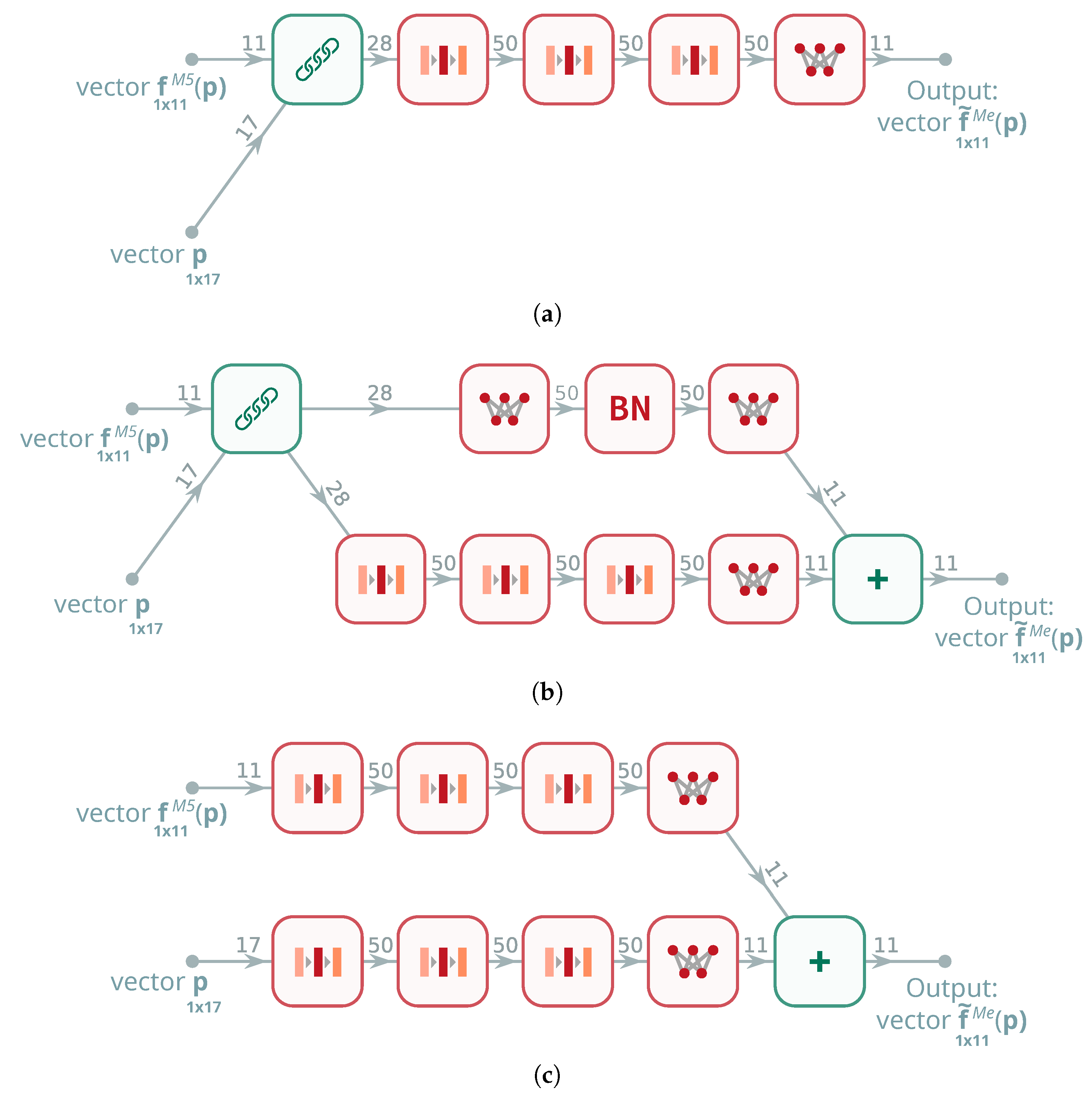
Two architectural realizations of the primary network were examined (Figure 6a,b). The first (Figure 6a, hereafter DNN) is a conventional fully connected multilayer deep neural network, and this baseline leverages depth to capture cross-feature interactions while remaining simple and robust.

The second design (Figure 6b, hereafter LNL) explicitly separates linear and nonlinear processing within each block to better model mappings that decompose into an additive linear trend plus a nonlinear residual. This decomposition strengthens the network’s ability to represent responses that are well approximated by a linear component modulated by a structured nonlinear correction (e.g., stiffness-weighted trends with geometry- and angle-dependent residuals).

For completeness, a third variant was considered in which the $\mathbf{p}$ and $f^{\mathcal{M}5}$ transformations are realized by two separate subnetworks $N_{\mathbf{p}}$ and $N_{f^{\mathcal{M}5}}$ operating in parallel on different inputs (Figure 6c, hereafter 2NETS), with predictions combined additively only at the output:

$${\widehat{\mathbf{f}}}^{\mathcal{M}e}=N_{f^{\mathcal{M}5}}\left(f^{\mathcal{M}5}\right)+N_{\mathbf{p}}\left(\mathbf{p}\right).$$

Although conceptually appealing, this configuration did not yield consistent advantages under the fixed training budget and is therefore reported only for completeness.

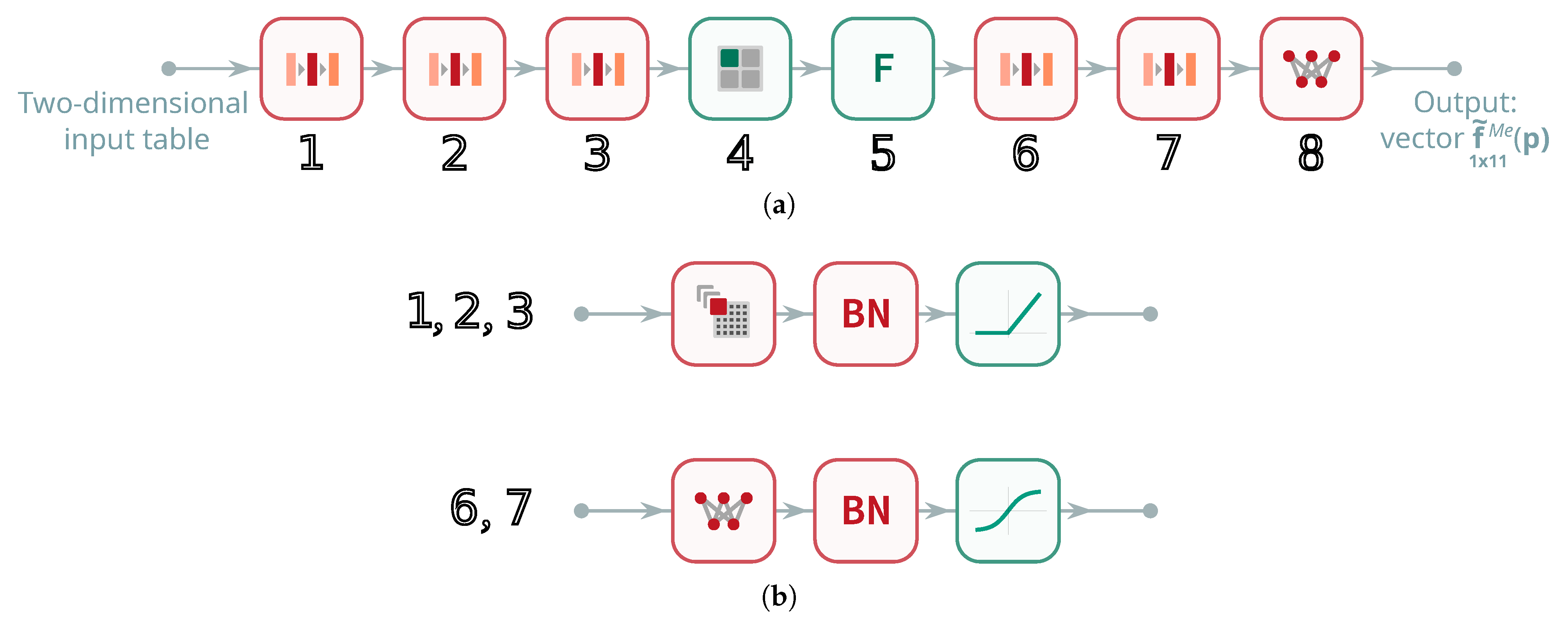
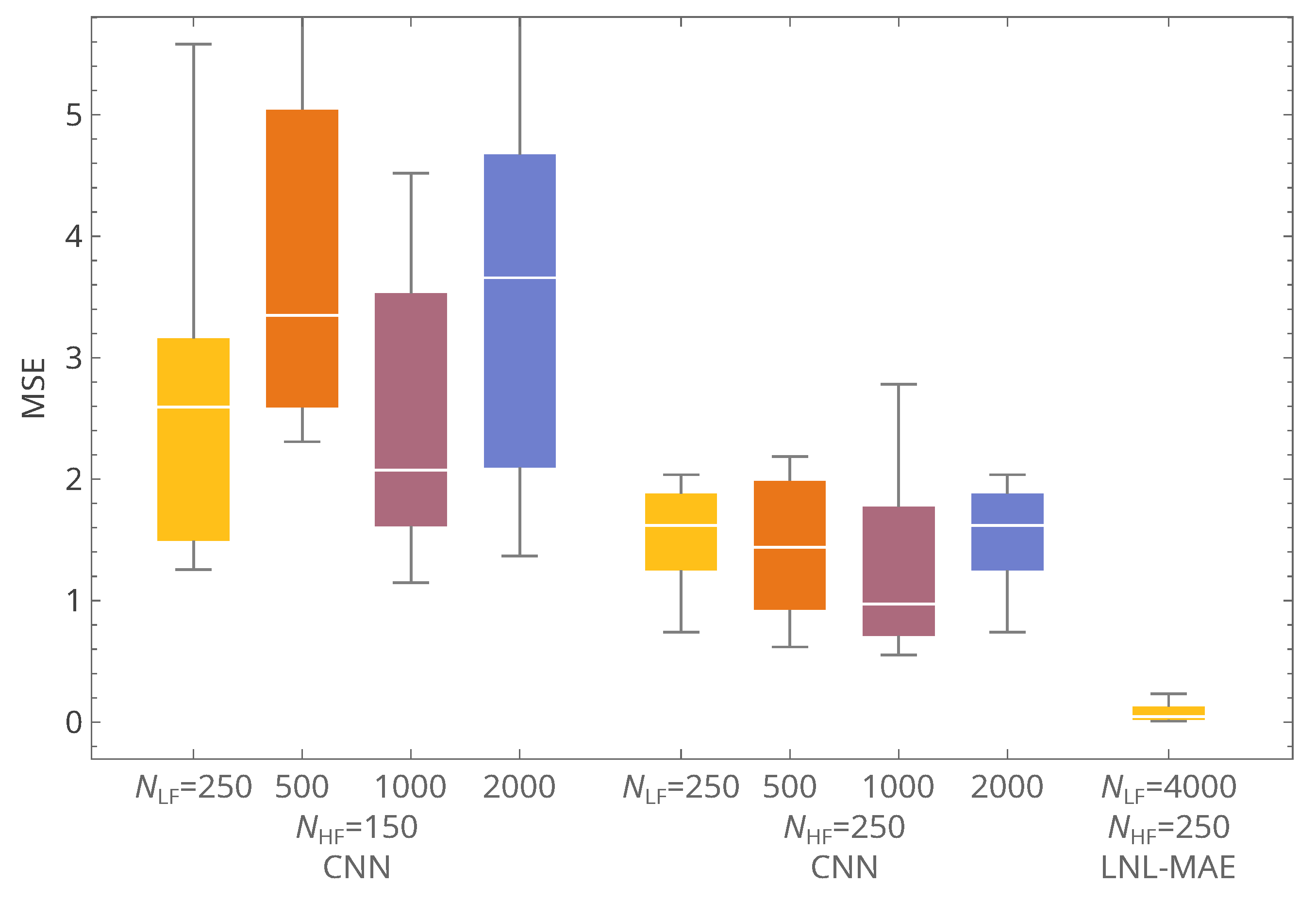
In addition to the DNN, LNL, and 2NETS configurations, a convolutional neural network (CNN) was also tested (Figure 7). The CNN replaces the fully connected layers with convolutional blocks designed to capture local correlations between input features. While such architectures are highly effective in image processing tasks, their advantage is less pronounced for tabular, mixed-type input vectors such as those considered here. In practice, the CNN exhibited consistently weaker accuracy than both the DNN and LNL architectures and was therefore not pursued further in the optimization studies.

The input data to the CNN are organized as two-dimensional tables. In each i-th input table, where $i=1,\dots ,N_{\mathrm{HF}}$, there are four meta-columns: ${\mathbf{p}}_{\mathrm{LF}}$, ${\mathbf{f}}^{M5}\left({\mathbf{p}}_{\mathrm{LF}}\right)$, ${\mathbf{p}}_{\mathrm{HF},i}$, and ${\mathbf{f}}^{Me}\left({\mathbf{p}}_{\mathrm{HF},i}\right)$, with a total number of $N_{\mathrm{LF}}$ rows. For the first two columns, ${\mathbf{p}}_{\mathrm{LF}}$ and ${\mathbf{f}}^{M5}\left({\mathbf{p}}_{\mathrm{LF}}\right)$, the tabular values in the j-th row are ${\mathbf{p}}_{\mathrm{LF},j}$ and ${\mathbf{f}}^{M5}\left({\mathbf{p}}_{\mathrm{LF},j}\right)$, respectively, where $j=1,\dots ,N_{\mathrm{LF}}$. With regard to the last two columns, the values ${\mathbf{p}}_{\mathrm{HF},i}$ and ${\mathbf{f}}^{Me}\left({\mathbf{p}}_{\mathrm{HF},i}\right)$ remain constant across all rows in the i-th table.

2.5.3. Variant 2—Cascaded HF Emulator + Pseudo-Experimental Mapper (Two-Network Ensemble)

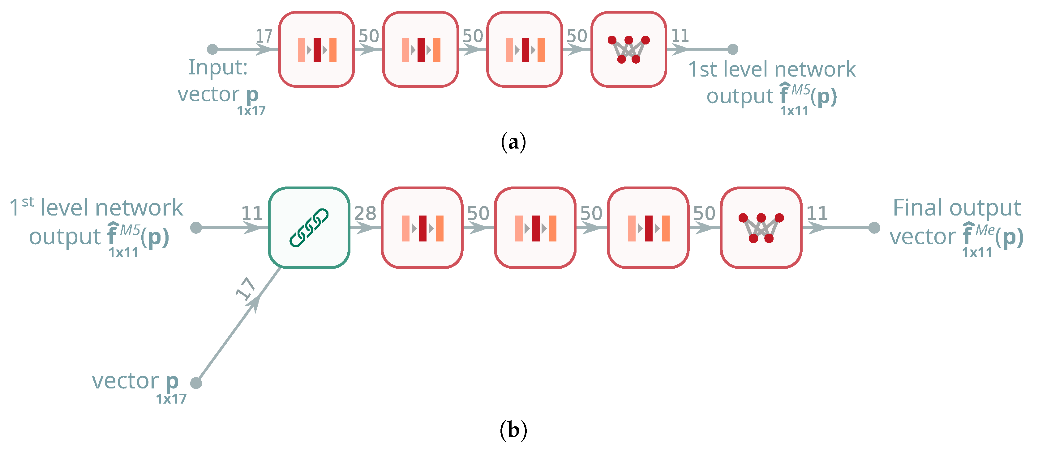
During optimization, the evaluator is a pair of neural networks queried in sequence, with no FEM calls in the loop (Figure 8). The first network $R_{\eta }$ takes the design vector $\mathbf{p}$ and returns a vector of eleven pseudo-$\mathcal{M}$5 frequencies,

$${\widehat{\mathbf{f}}}^{\mathcal{M}5}\left(\mathbf{p}\right)=R_{\eta }\left(\mathbf{p}\right)\approx {\mathbf{f}}^{\mathcal{M}5}\left(\mathbf{p}\right),$$

(10)

i.e., it emulates the low-fidelity model $\mathcal{M}$5. The second network $S_{\theta }$ receives both the design vector and the output of $R_{\eta }$ and predicts the pseudo-experimental targets,

$${\widehat{\mathbf{f}}}^{\mathcal{M}e}\left(\mathbf{p}\right)=S_{\theta }\left(\mathbf{p},{\widehat{\mathbf{f}}}^{\mathcal{M}5}\left(\mathbf{p}\right)\right)\approx {\mathbf{f}}^{\mathcal{M}e}\left(\mathbf{p}\right),$$

(11)

where ${\mathbf{f}}^{\mathcal{M}e}$ is defined by the mapping in Equation (2). Training proceeds in two steps with teacher forcing: (i) fit $R_{\eta }$ on LF data to approximate ${\mathbf{f}}^{\mathcal{M}5}\left(\mathbf{p}\right)$; and (ii) fit $S_{\theta }$ on pairs $\left(\mathbf{p},{\mathbf{f}}^{\mathcal{M}5}\left(\mathbf{p}\right)\right)$ to approximate ${\mathbf{f}}^{\mathcal{M}e}\left(\mathbf{p}\right)$.

At application time, the GA uses only the neural ensemble $(R_{\eta },S_{\theta })$ to evaluate $g_f(·)$; the cost $g_c(·)$ remains analytic. This cascade preserves the structure “LF → pseudo-experiment,” improves data efficiency, and cleanly separates modeling roles, while acknowledging and controlling potential error propagation from the first to the second stage.

2.6. Rationale and Computational Footprint

The three variants are designed to disentangle accuracy–cost trade-offs under strict limits on high-fidelity (HF) evaluations. Let $N_{\mathrm{HF}}$ and $N_{\mathrm{LF}}$ denote the numbers of HF ($\mathcal{M}1$ and in consequence $\mathcal{M}$e($\mathcal{M}1$)) and low-fidelity (LF, $\mathcal{M}$5) simulations used to train the surrogate(s). With the $\mathcal{M}$5 element size four times larger than $\mathcal{M}1$, one LF run costs approximately $1/4^2$ of an HF run, while its discretization error grows on the order of $4^4$ [28]. We therefore report an HF-equivalent training cost:

$${\mathcal{C}}_{\mathrm{eq}}=N_{\mathrm{HF}}+{\displaystyle \frac{N_{\mathrm{LF}}}{16}}.$$

(12)

The adopted dataset sizes and fidelity ratios were also justified in prior research. A heuristic rule was proposed, namely, that the number of training patterns (in thousands) should be approximately one-fourth to one-fifth of the number of design variables [38], which, for the current 17 variables, corresponds to about 4000 low-fidelity samples. In later works, we demonstrated that supplementing these with about 250 high-fidelity samples ensures a good balance between accuracy and cost [28,29]. The choice of the high-fidelity finite element mesh was validated by convergence analyses [38], while the low-fidelity mesh was selected based on the error–time trade-off.

Variant 0 (HF-only) requires a dense HF dataset to generalize over the 17-dimensional design space. In line with prior experience, several thousand samples are needed; to fix ideas, set $N_{\mathrm{HF}}=4000$, which gives ${\mathcal{C}}_{\mathrm{eq}}=4000$. Using the per-run CPU time of the HF model reported in Section 2.2, one HF-equivalent unit corresponds to $888.36$ s of CPU time. Thus, a budget of ${\mathcal{C}}_{\mathrm{eq}}=4000$ amounts to $4000\times 888.36\mathrm{s}\approx 41.13$ days of CPU time.

Variant 1 (MF-trained, auxiliary refinement) replaces most HF labels with refined LF labels produced by the auxiliary network. Using, for illustration, $N_{\mathrm{HF}}=250$ paired with $N_{\mathrm{LF}}=4000$ (with 250 LF samples co-located with the HF designs) yields

$${\mathcal{C}}_{\mathrm{eq}}\approx 250+{\displaystyle \frac{4000}{16}}=500,$$

(13)

i.e., an order-of-magnitude reduction in HF-equivalent cost. Although raw LF errors scale unfavorably with mesh coarsening, the refinement learned by the auxiliary network suppresses this bias before training the primary evaluator. On the same CPU-time scale, ${\mathcal{C}}_{\mathrm{eq}}=500$ entails $\approx 5.14$ days of HF-equivalent simulation time for pattern generation.

Variant 2 (cascaded emulator + mapper) distributes learning across two networks: an LF-trained emulator and an HF-trained mapper to pseudo-experimental targets. Its HF-equivalent cost follows Equation (12) with the budgets assigned to the two stages. Matching the illustrative budgets of Variant 1 leads to a comparable ${\mathcal{C}}_{\mathrm{eq}}\approx 500$, while allowing even larger $N_{\mathrm{LF}}$ at negligible HF-equivalent overhead to reduce variance. The cascade preserves the LF$\to$ $\mathcal{M}e$ structure at inference, offering a complementary accuracy–cost trade-off relative to the offline-refinement route. Accordingly, with ${\mathcal{C}}_{\mathrm{eq}}\approx 500$, the HF-equivalent simulation time for dataset generation is again $\approx 5.14$ days.

In addition to simulation time, one must account for network training and testing. With three NVIDIA A30 GPUs acceleration (each NVIDIA A30 with one GA100 graphics processor unit, 24 GB memory, 1440 MHz, 3584 shading and 224 tensor cores) (NVIDIA, Santa Clara, CA, USA), the times per run were as follows: Variant 0—a single network trained in ≈5 min; repeated 30 times, this totals $\approx 2.5$ h. Variant 1—two networks, auxiliary $\approx 1.5$ min and primary $\approx 5$ min per repeat; for 30 repeats, ≈3.25 h. Variant 2—identical training profile to Variant 1, i.e., ≈3.25 h for 30 repeats. The sole exception concerns models trained with an arcsinh-based loss, for which convergence was several times slower than with MSE/MAE under the same stopping criteria. After adopting surrogates, the GA optimization time became negligible relative to FEM simulation time. A final FEM-based verification of the returned designs added a comparable overhead across all settings; the verification stage required $\approx 31$ h.

Because the FEM simulations were executed exclusively on CPUs, whereas the neural-network training/testing was executed exclusively on a GPU, adding “CPU time” and “GPU time” into a single total is neither justified nor meaningful. We therefore report them separately (HF-equivalent CPU time for dataset generation and GPU wall time for network training). If, despite this caveat, one wished to approximate a single aggregate, the CPU time should first be normalized by the number of concurrently used threads (≈20 in our runs) to obtain a comparable per-device wall time; however, such an aggregate would still have limited interpretability.

In summary, the variants benchmark (i) a classical HF-only baseline,(ii) an MF pipeline that converts abundant LF into pseudo-HF labels for a single evaluator, and (iii) an MF cascade that factors the mapping and can exploit vast LF corpora—each eliminating FEM calls during optimization but differing in where computational effort is spent and how LF information is leveraged.

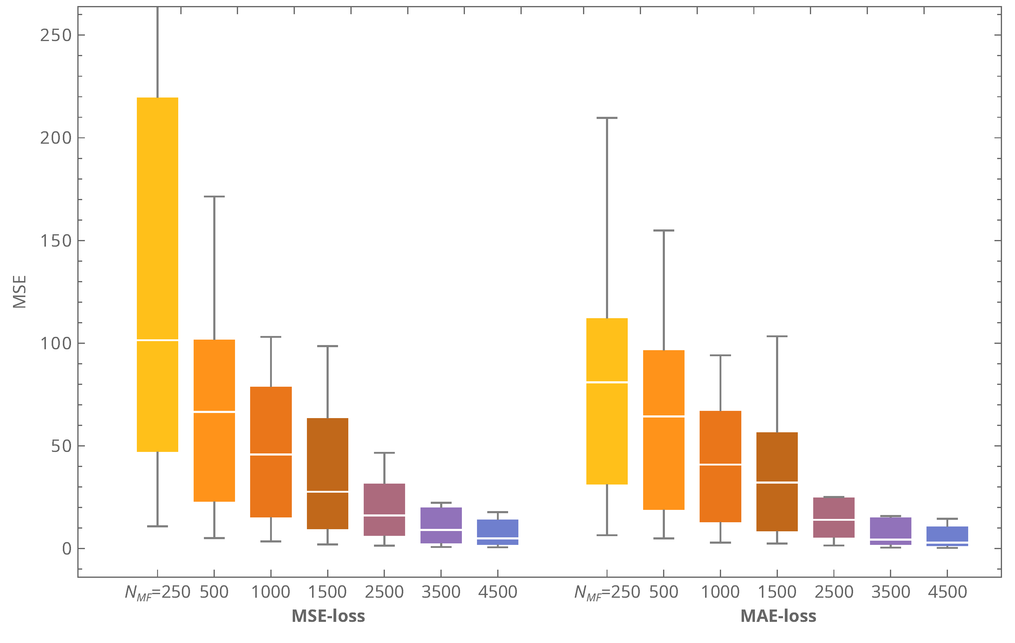
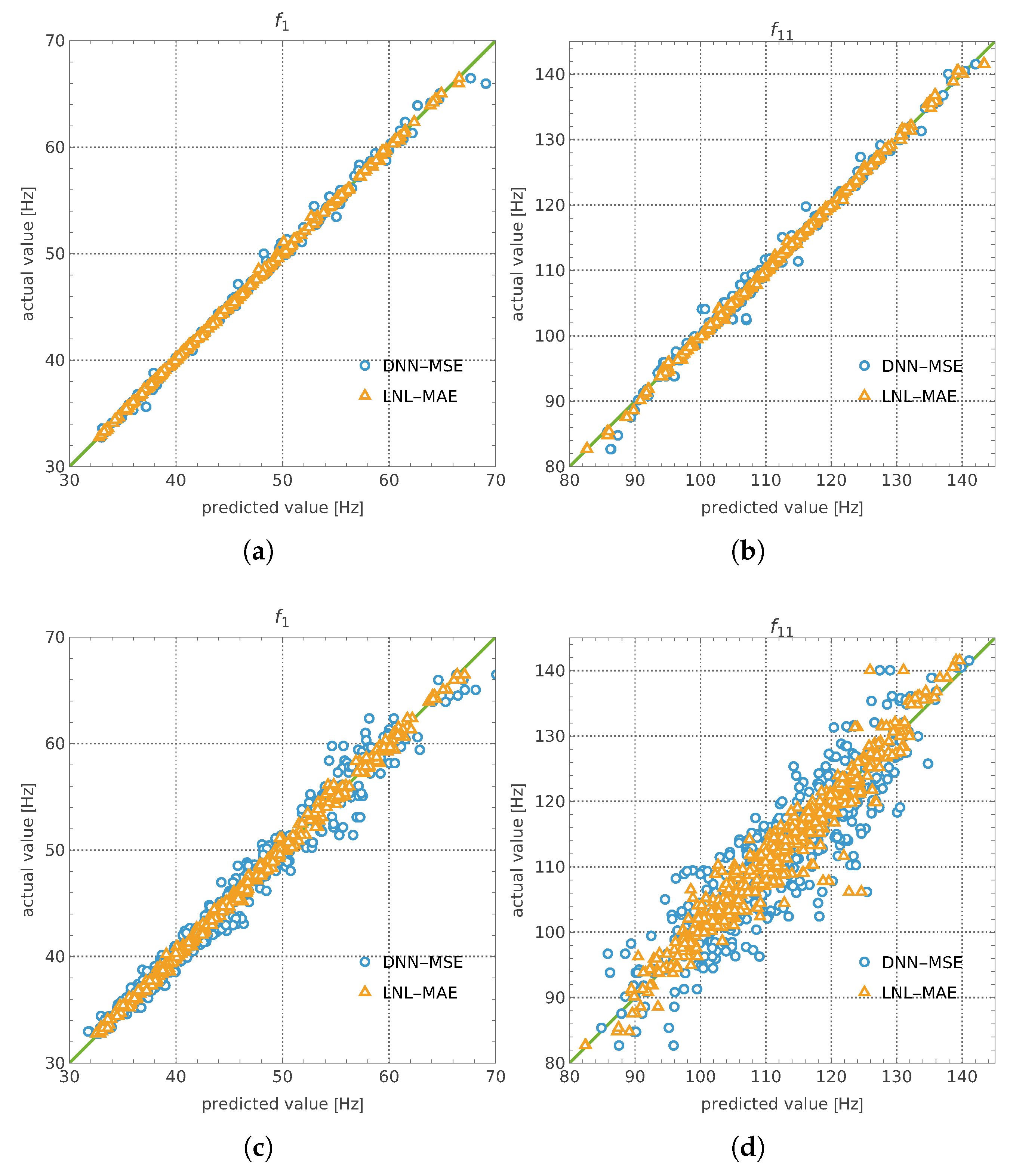
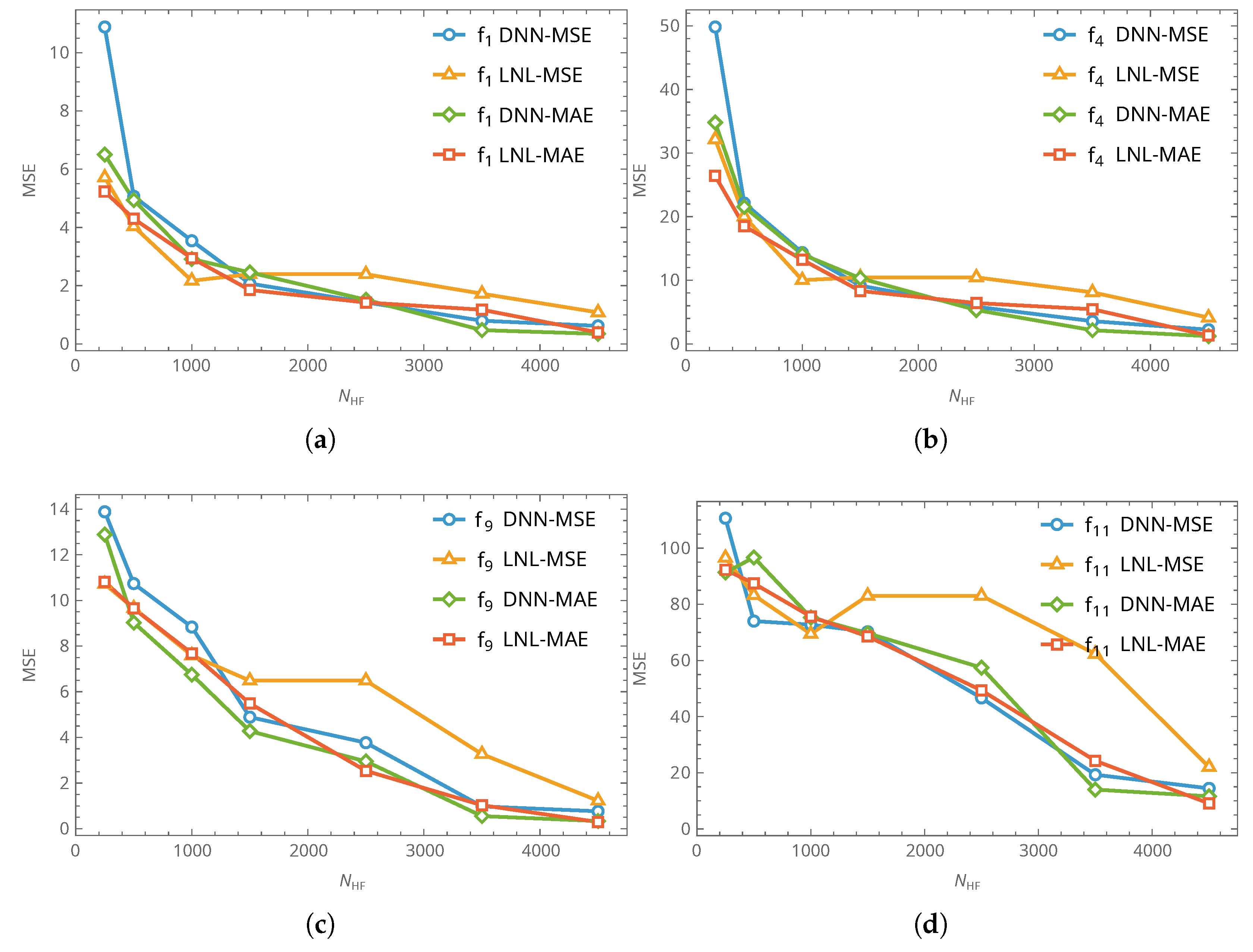
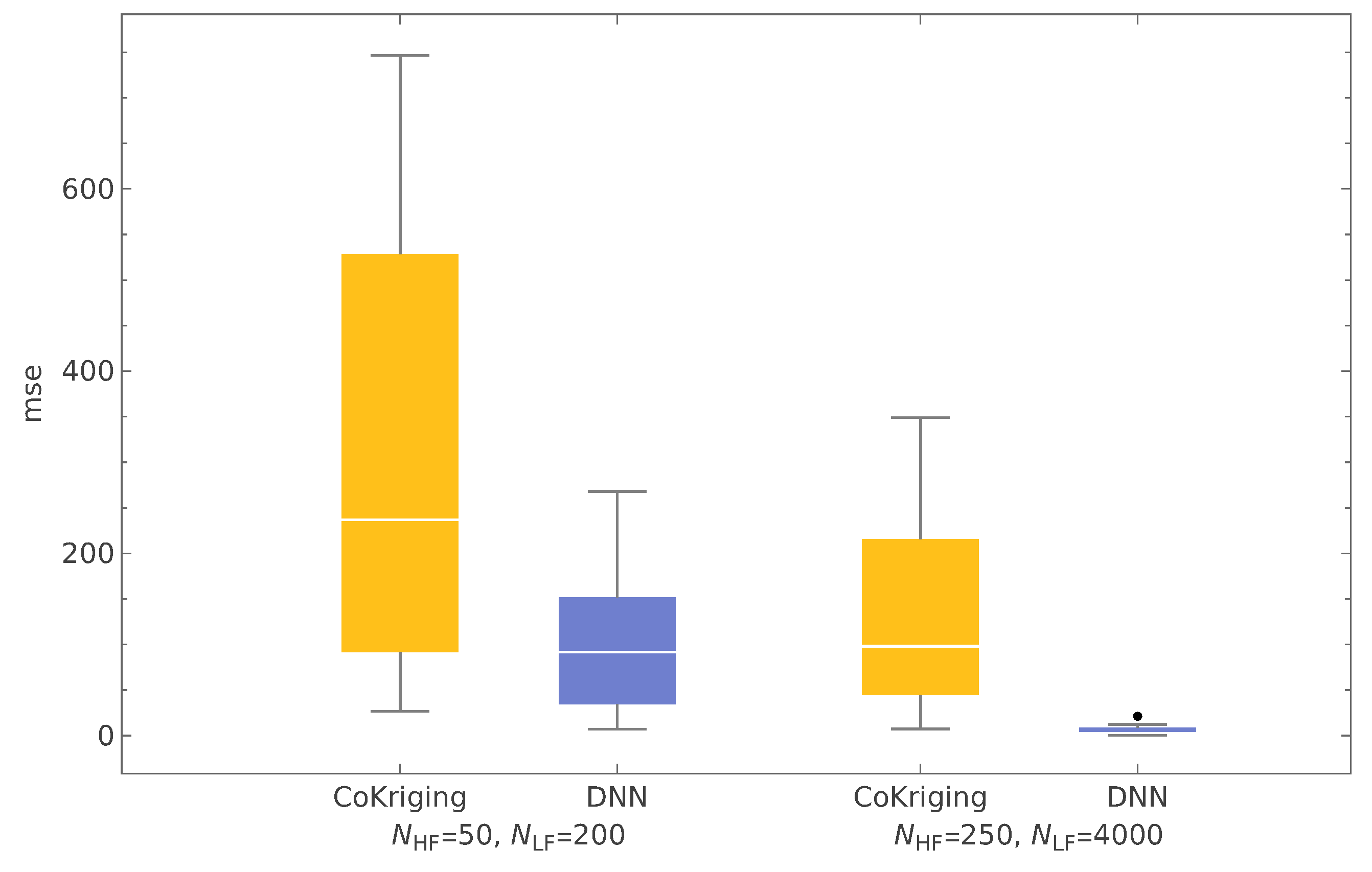
In the present hyperboloidal shell setting (see Figure 2a–c), relying solely on Variant 0 is not only computationally onerous but also degrades surrogate accuracy: the SM validation error (MSE) is two orders of magnitude larger than for an otherwise comparable cylindrical case (see Figure 2d). Two factors are dominant. First, the design space is higher-dimensional (17 versus 16 variables), which raises sample complexity and demands substantially more HF labels to achieve the same generalization level; the additional variable is a geometric descriptor—the hyperboloid depth parameter d—absent in the cylindrical baseline. Second, accurate identification and tracking of the target mode shapes across designs is markedly harder for the hyperboloid: curvature reversal and stronger meridional coupling induce modal veering and near-degeneracies, making the mapping from FE eigenpairs to the fixed set of eleven target modes more error-prone. Even rare misassignments (label noise) propagate into the surrogate’s loss, inflate MSE, and reduce fidelity near the resonance-avoidance band.

Recognizing these limitations, we treat the hyperboloidal case as a deliberately stringent benchmark and leverage the MF strategies (Variants 1–2) to counteract both issues: they reduce the HF labeling burden while using LF-informed refinement/cascades to stabilize learning under label noise and heightened nonlinearity. This choice tests whether multi-fidelity design—not mere model capacity—can restore predictive accuracy and, in turn, improve Pareto-front quality at a fraction of the HF-equivalent cost.

We analyzed three surrogate configurations, summarized in

Table 2. Variants of surrogate models; network symbols are illustrated in Figure 6 and Figure 7.

	Data for Auxiliary SM	Neural Networks	Data for Primary SM	Neural Networks
Variant 0	—	—	Single Fidelity	DNN
Variant I	Multi Fidelity	DNN	Single Fidelity	DNN
		LNL		LNL
		2NETS
		CNN
Variant II	Multi Fidelity	DNN	Multi Fidelity	DNN
		LNL		LNL
		2NETS

. All variants predict the vector of selected natural frequencies used in $g_f(·)$; the cost $g_c(·)$ is evaluated analytically from material choices and geometry; hence, it is not surrogated. The backbone family, optimizer, and training budget are kept identical across variants; only the data sources and training protocols differ.

2.7. Neural Networks Applied

Deep neural networks are used as the surrogate backbone because they efficiently approximate highly nonlinear mappings from the mixed discrete–continuous design vector to the eleven target frequencies while remaining inexpensive at query time [13,14]. Inputs comprise standardized continuous features (geometry and ply angles) and one-hot encodings for plywise material choices; depending on the variant, auxiliary signals are concatenated, so the effective input dimensionality is either 17 (design only), 28 (design+${\mathbf{f}}^{\mathcal{M}5}$). Hidden layers employ nonlinear activations, and the output head is linear to predict all eleven frequencies jointly, allowing the model to exploit cross-output correlations. Regularization includes weight decay, dropout, and batch normalization; optimization uses mini-batches with gradient clipping and an early-stopping criterion on a held-out validation split.

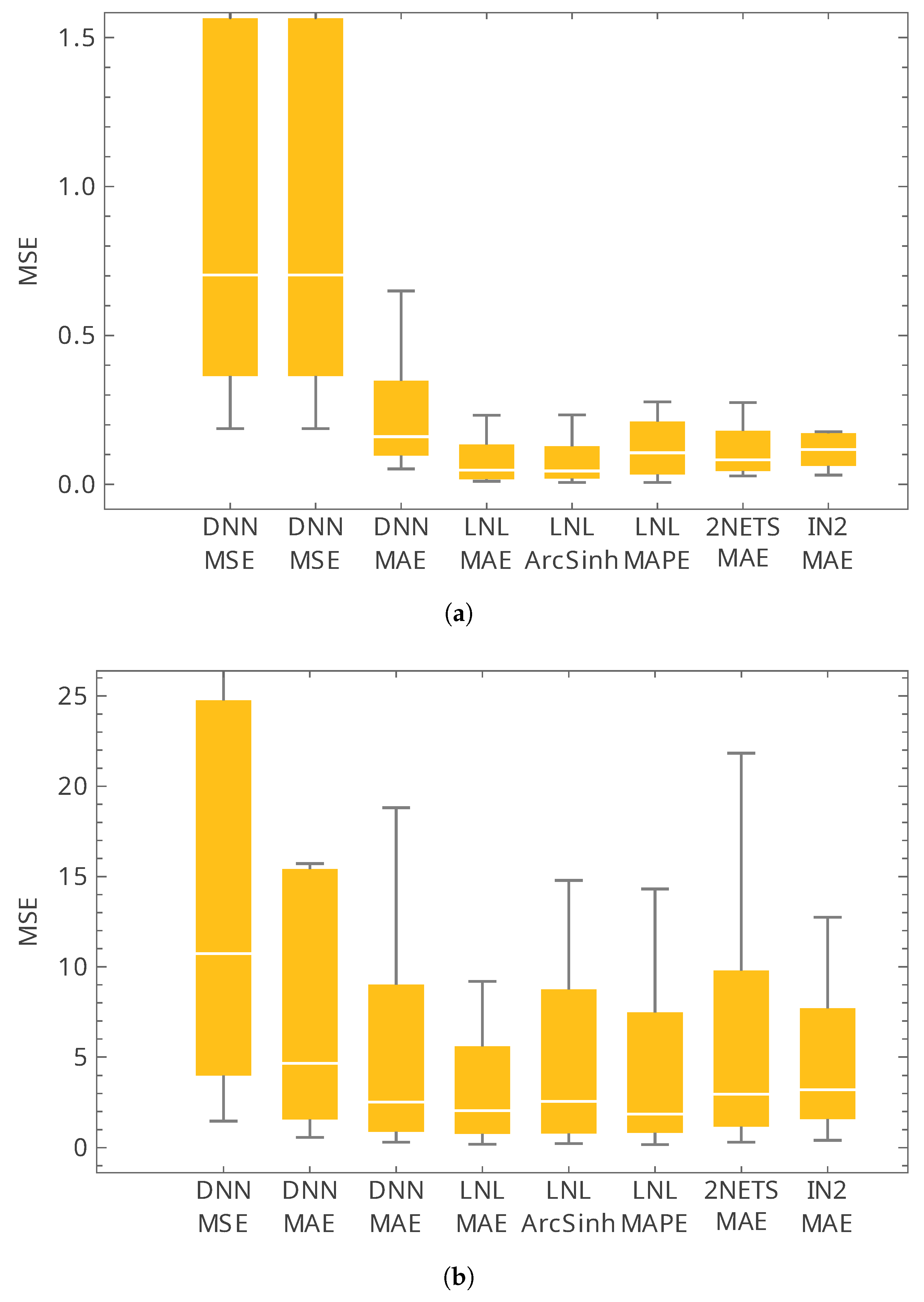
To avoid biasing results toward a specific architecture or optimizer, we performed a controlled hyperparameter sweep covering network depth (4–8 layers), width (20–100 units per layer), and three optimizers (ADAM, RMSProp, and SGD), together with several activation functions (ReLU, tanh, and sigmoid; softmax was considered only in auxiliary classification branches when applicable). For the loss, we compared MSE and MAE with more robust alternatives, namely the mean absolute percentage error (MAPE) and an error metric based on the inverse hyperbolic sine transformation (ArcSinh-based error), in order to accommodate scale differences across modes. Overall, performance differences were found to depend primarily on the fidelity strategy (single- vs. multi-fidelity data usage and network coupling) rather than on incidental architectural or optimizer choices.

The details of the examined approaches are summarized in

Table 3. Architectures, algorithms, activation functions, and methods.

Component	Settings / Values
Network architecture	$I=\{17,28,39\}$
$I-H^{(·)}-O$	$N_L=\{4,5,6,7,8\}$
	$H^{(·)}=\{20,30,40,50,75,100\}$
	$O=11$
Learning algorithms	ADAM
	RMSProp
	SGD
Regularization methods	Early stopping
	$L_2$ Regularization
	Dropout
	Batch normalization
Activation functions	softmax
	tanh
	ReLU
	sigmoid
Loss functions	MSE
	MAE
	arcsinh
	MAPE

.

2.8. Non-Dominated Sorting Genetic Algorithm II in Brief

The Non-Dominated Sorting Genetic Algorithm II is a population-based, elitist evolutionary method widely used for multi-objective optimization [3]. It maintains a set of candidate solutions and iteratively improves both convergence to, and coverage of, the Pareto front by combining fast non-dominated sorting with a crowding-distance diversity measure.

The algorithm begins by sampling an initial population $P_0$ of size N from the decision space $\mathbb{P}$ and evaluating the corresponding objective vectors $\mathbf{g}\left(\mathbf{p}\right)$. At each generation t, an offspring set $Q_t$ of size N is created using tournament selection guided by Pareto rank and crowding distance, followed by simulated binary crossover and polynomial mutation or related operators [44]. The objective values of $Q_t$ are then evaluated and combined with the parent population to form $R_t=P_t\cup Q_t$. Fast non-dominated sorting is applied to $R_t$ to identify fronts $F_1,F_2,\dots$, and crowding distance is used within each front to estimate local solution density [3]. The next population $P_{t+1}$ is filled with entire fronts in order of rank until the size limit is reached; if the last front does not fit, the most widely spaced solutions are selected based on crowding distance.

This process repeats until the generation budget or another stopping criterion is met, and the first front $F_1$ of the final population is returned as an approximation of the Pareto-optimal set [45]. By jointly addressing convergence (toward Pareto optimality) and diversity (distribution along the front), with an overall sorting complexity of $\mathcal{O}\left(M{N}^2\right)$ for M objectives [3], NSGA-II provides a robust default for mixed discrete–continuous design spaces and rugged, multi-modal response landscapes.

3. Results

3.1. Accuracy of Surrogate Models: Variant 0 (HF-Only Surrogates)

Variant 0 evaluates a single SM (with a DNN backbone) trained exclusively on high-fidelity (HF) data pairs $(\mathbf{p};{\mathbf{f}}^{\mathcal{M}e}\left(\mathbf{p}\right))$, where ${\mathbf{f}}^{\mathcal{M}e}$ denotes the pseudo-experimental frequency vector obtained from $\mathcal{M}1$ through the nonlinear mapping $\mathcal{M}e(·)$ (see Equation (2)). Model quality is assessed against the pseudo-experimental responses computed directly from $\mathcal{M}1$, which represent the FEM “ground truth” for this baseline.

The accuracy of the SM is quantified by the mean squared error (MSE) between predictions and $\mathcal{M}e(·)$ references on the held-out test set. For a single design vector $\mathbf{p}$,

$$\mathrm{MSE}\left(\mathbf{p}\right)={\displaystyle \frac{1}{11}}\sum _{k\in \mathcal{S}}{\left({\widehat{f}}_k^{\mathcal{M}e}\left(\mathbf{p}\right)-f_k^{\mathcal{M}e}\left(\mathbf{p}\right)\right)}^2,$$

(14)

and the reported score corresponds to the average (with dispersion measures) over all test samples. As in the training stage, natural frequencies are consistently standardized prior to error computation.

The SM was trained on HF-only datasets of increasing size:

$$N_{\mathrm{HF}}\in \{250,500,1000,1500,2500,3500,4500\}.$$

For each training size, two surrogates were constructed differing only in the loss function used during training:

• MSE loss (mean squared error);
• MAE loss (mean absolute error).

Regardless of the loss function, performance was always evaluated in terms of test-set MSE with respect to the pseudo-experimental FEM responses.

The results are summarized in Figure 9, which presents the outcomes in the form of box-and-whisker plots. For each training size and loss function, the central mark indicates the median value, the box edges represent the interquartile range (25th to 75th percentile), and the whiskers extend to the minimum and maximum observed values across repeated runs. This visualization highlights not only the central tendency of prediction errors but also their variability, providing a concise statistical summary of the surrogate accuracy under different training regimes.

3.1.1. Scaling with HF Training SIZE

Test-set MSE decreases monotonically with increasing $N_{\mathrm{HF}}$, confirming that additional HF samples improve surrogate generalization. The largest reductions in error occur when moving from very small budgets (250–500 samples) to medium-size datasets (1000–1500 samples). Beyond this range, further enlarging the training set yields only incremental improvements, with markedly reduced error reduction per additional HF sample. This regime of diminishing returns is typical in high-dimensional supervised learning: once the dominant nonlinear trends are captured, remaining discrepancies are due to finer-scale variations, occasional mode-tracking errors, or architectural limits, all of which require disproportionately larger data to correct. Consequently, purely HF-based surrogates become cost-inefficient at large $N_{\mathrm{HF}}$, motivating the use of multi-fidelity strategies to achieve comparable accuracy at reduced expense.

3.1.2. Effect of Loss Function

For smaller budgets ($N_{\mathrm{HF}}\le 1000$), surrogates trained with MAE loss consistently achieve lower test-set MSE than those trained with MSE loss. This reflects the greater robustness of MAE to outliers: by penalizing deviations linearly rather than quadratically, it prevents rare but large errors from dominating the training signal, a property especially valuable when only a handful of HF samples is available. As the dataset grows ($N_{\mathrm{HF}}\ge 2500$), the influence of outliers diminishes and the residuals become more Gaussian-like. Overall, however, the performance gap between the two losses becomes negligible at high budgets, indicating that data abundance reduces the importance of the chosen training objective.

3.1.3. Stability Across Seeds

The dispersion of test errors across repeated runs is substantial at low training budgets, where random initialization and small-sample effects strongly influence convergence. Different seeds may lead to noticeably different local minima, resulting in wide spreads of MSE values. As $N_{\mathrm{HF}}$ increases, this sensitivity diminishes: richer datasets provide broader coverage of the design space and reduce the impact of mislabeled or atypical samples, so most runs converge to similar-quality solutions. An additional observation is that MAE-trained models tend to show narrower error distributions at low budgets, again highlighting their robustness to outliers and random fluctuations. This stabilizing effect becomes less pronounced at larger $N_{\mathrm{HF}}$, where both losses yield comparably stable results.

3.1.4. Cost–Quality Trade-Off

While accuracy improves with increasing $N_{\mathrm{HF}}$, the computational expense grows linearly with the number of HF simulations. The steepest accuracy gains are realized early, but past approximately $N_{\mathrm{HF}}=1500$ the improvement per unit of HF cost is minimal. This imbalance highlights the inefficiency of relying solely on large HF datasets: the marginal benefit does not justify the additional FEM computations. Instead, moderate HF budgets should be combined with abundant LF data to maximize accuracy per unit cost. Variants 1 and 2, introduced in the following sections, implement this multi-fidelity strategy and are expected to deliver HF-level predictive performance at only a fraction of the HF-equivalent training cost.

3.2. Accuracy of Surrogate Models: Variant 1 (MF-Trained with Auxiliary Refinement)

In Variant 1, the auxiliary network consistently achieves very high accuracy due to its enriched input representation including all 11 frequencies. By contrast, the primary network is less accurate, which is why the following analysis focuses primarily on its results. As an illustration, Figure 10 compares predictions from both networks for a representative case. The plots adopt a standard format widely used in neural network evaluation: the horizontal axis shows the predicted values, while the vertical axis shows the corresponding actual (reference) values, and each sample is represented by one point. Points closer to the diagonal line $x=y$ indicate higher accuracy. The figure clearly demonstrates the superior performance of the auxiliary network, with the errors of the primary network being approximately fifteen times larger. The comparison is presented for frequency $f_1$ (the easiest to approximate) and frequency $f_{11}$ (the most challenging).

Having illustrated the relative accuracy of the auxiliary and primary networks in Figure 10, we now turn to a broader comparison of architectural choices. Variant 1 employs both HF and LF data, with the auxiliary network $R_{\eta }$ generating refined pseudo-experimental labels that enlarge the effective training corpus. We compare two realizations of the auxiliary network: (i) DNN, a conventional fully connected network (Figure 6a), and (ii) LNL, a block-wise design that explicitly separates linear and nonlinear processing paths (Figure 6b). To improve clarity, the comparison is reported for a subset of selected natural frequencies (e.g., $f_1$, $f_4$, $f_9$, and $f_{11}$), representative of both the more stable and the more challenging modes within the set $\mathcal{S}$.

The same HF budgets as in Variant 0 are examined,

$$N_{\mathrm{HF}}\in \{250,500,1000,1500,2500,3500,4500\}.$$

In each case, two representative configurations are tested during training: a conventional DNN trained with MSE loss and an LNL architecture trained with MAE loss. Predictive accuracy is consistently evaluated in terms of test-set MSE against the FEM-based pseudo-experimental reference. The corresponding results are summarized in Figure 11.

3.2.1. Effect of Architectural Choice

At small HF budgets, which are the most critical for the present study, the linear–nonlinear (LNL) decomposition markedly outperforms the conventional fully connected architecture. The benefit is especially visible for modes $f_9$ and $f_{11}$, where isolating a dominant linear trend from a nonlinear residual stabilizes the mapping and reduces errors. For the simpler modes $f_1$ and $f_4$, whose FEM responses exhibit less variability, the difference between architectures narrows, and once $N_{\mathrm{HF}}$ exceeds about 1000, both achieve comparable accuracy.

3.2.2. Effect of Loss Function

For the smallest training budgets ($N_{\mathrm{HF}}=250$ and 500), models trained with MAE loss consistently yield lower test-set MSE than those trained with MSE loss. This echoes the robustness to outliers already observed in Variant 0 and indicates that the stabilizing influence of MAE is particularly valuable when only a limited number of HF samples are available. As $N_{\mathrm{HF}}$ increases, however, the discrepancy between the two loss functions diminishes. By $N_{\mathrm{HF}}\ge 1500$, both losses deliver similar performance, suggesting that data sufficiency reduces the impact of the loss choice.

3.2.3. Mode-Dependent Improvements

Accuracy improvements are strongly mode-dependent. For stable modes such as $f_1$ and $f_4$, the test errors change only marginally with growing $N_{\mathrm{HF}}$, and the role of multi-fidelity training is limited. In contrast, for more challenging modes such as $f_9$ and $f_{11}$, the LF-informed refinement continues to provide clear benefits even at larger HF budgets. These cases demonstrate that Variant 1 not only reduces HF requirements but also enhances robustness in regions of the spectrum that are intrinsically difficult to approximate.

The results show that Variant 1 successfully reduces the dependency on large HF datasets. At the low HF budgets most relevant in practice, combining LF refinement with LNL architectures and MAE-loss training yields the best overall accuracy. This confirms the benefit of explicitly modeling additive linear and nonlinear components and demonstrates that multi-fidelity pipelines can stabilize learning for difficult modes while preserving efficiency for simpler ones.

Having analyzed Figure 11, we now turn to a broader comparison that considers several specific loss–architecture pairs under fixed HF/LF budgets. Within Variant 1 (MF-trained with auxiliary refinement), we examined these combinations while keeping the HF/LF corpus sizes fixed to the adopted budgets ($N_{HF}=250$, augmented with a large LF pool, $N_{LF}=4000$, refined by $R_{\eta }$). As in the previous sections, accuracy is reported as the test-set MSE with respect to the pseudo-experimental FEM reference.

We considered the following configurations of Variant 1 (notation consistent with Figure 6):

• DNN — Trained with either MSE loss or MAE loss.
• LNL — Trained with MAE loss, with arcsinh-based error (LNL–ArcSinh), or with mean absolute percentage error (LNL–MAPE).
• 2NETS — Trained with MAE loss.
• IN2 — A DNN architecture with extended inputs: In addition to the design vector $\mathbf{p}$ and the LF response vector ${\mathbf{f}}^{\mathcal{M}5}$, it also receives the response vector ${\mathbf{f}}^{\mathcal{M}10}$. The latter corresponds to an auxiliary, coarser low-fidelity model with element size $h=10$ cm, considered only in this configuration and not used elsewhere in the study.

The weakest accuracy (see Figure 12a) is obtained by DNN–MSE; DNN–MAE performs better but still falls short compared to the other options. The best results are delivered by LNL–MAE and LNL–ArcSinh. Although both achieve comparable test-set accuracy, the arcsinh-based loss requires substantially longer training to converge. Given this added computational cost and the only marginal improvement it provides, the balance tips in favor of LNL–MAE as the more practical and cost-effective choice. The 2NETS and IN2 configurations perform consistently at an intermediate level: occasionally competitive on specific modes but not dominant on average. Similarly, the use of the MAPE loss function does not yield meaningful improvements.

Panel (b) of Figure 12 presents the results obtained with the primary network across the same set of loss–architecture combinations as in panel (a). Each bar in (b) corresponds to the final outcome of an auxiliary–primary pair, where the auxiliary performance is shown in panel (a) and the primary performance in panel (b). The comparison clearly indicates that the most accurate results are achieved when both networks in the pair (auxiliary and primary) adopt the LNL architecture trained with MAE loss. This combination consistently outperforms all others, confirming that the explicitly modeled linear and nonlinear components in both networks provide the most effective refinement of low-fidelity data and the most reliable surrogate predictions. The numerical values corresponding to the graphical results in panel (b) are summarized in

Table 4. Test-set MSE values for the primary network across different loss–architecture configurations in Variant 1. The results correspond to the graphical comparison shown in Figure 12b.

${\displaystyle \frac{\mathbf{Auxiliary}}{\mathbf{Primary}}}$	Min	25%	Median	75%	Max
${\displaystyle \frac{\mathrm{DNN}–\mathrm{MSE}}{\mathrm{DNN}–\mathrm{MSE}}}$	1.46	4.00	10.69	24.80	35.40
${\displaystyle \frac{\mathrm{DNN}–\mathrm{MSE}}{\mathrm{DNN}–\mathrm{MAE}}}$	0.56	1.56	4.62	15.37	15.68
${\displaystyle \frac{\mathrm{DNN}–\mathrm{MAE}}{\mathrm{DNN}–\mathrm{MAE}}}$	0.30	0.88	2.50	9.00	18.84
${\displaystyle \frac{\mathrm{LNL}–\mathrm{MAE}}{\mathrm{LNL}–\mathrm{MAE}}}$	0.19	0.76	2.04	5.57	15.37
${\displaystyle \frac{\mathrm{LNL}–\mathrm{ArcSinh}}{\mathrm{LNL}–\mathrm{ArcSinh}}}$	0.23	0.79	2.53	8.76	14.75
${\displaystyle \frac{\mathrm{LNL}–\mathrm{MAPE}}{\mathrm{LNL}–\mathrm{MAPE}}}$	0.16	0.83	1.85	7.45	14.29
${\displaystyle \frac{2\mathrm{NETS}–\mathrm{MAE}}{2\mathrm{NETS}–\mathrm{MAE}}}$	0.30	1.17	2.92	9.80	21.81
${\displaystyle \frac{\mathrm{IN}2–\mathrm{MAE}}{\mathrm{IN}2–\mathrm{MAE}}}$	0.41	1.59	3.20	7.67	12.74

.

For completeness, we also examined CNNs [46] as an alternative backbone for the surrogate in Variant 1 (applied to the auxiliary network) (see Figure 13; compare with the results in Figure 12a). This additional test confirmed that CNN-based surrogates deliver consistently lower accuracy than the fully connected or LNL designs. Given their weaker performance in the present setting, CNNs were not considered further in the study.

In addition, we verified a well-known surrogate modeling technique, namely, co-Kriging [6,20,25], again applied as a substitute for the auxiliary DNN in Variant 1. The corresponding results (see Figure 14) were clearly inferior to those obtained with neural-network-based surrogates, further confirming that deep architectures are the more suitable choice for the present problem class.

4. Final Optimization Results: Pareto Fronts and Indicators

Curriculum learning was applied to improve both surrogate accuracy and optimization outcomes. Figure 15 presents Pareto fronts obtained directly from the optimization runs for three settings: (a) Variant 1 with a DNN surrogate; (b) Variant 1 with an LNL surrogate; and (c) Variant 2. Each subfigure shows a series of Pareto fronts corresponding to successive CL loops. Although the fronts illustrate the progressive optimization process, the quality differences between successive stages of CL are subtle and, in many cases, extremely difficult—if not impossible—to distinguish visually.

For this reason, the same results are presented in an alternative form in Figure 16. Subfigure (a) reports the accuracy of the surrogate models (Variant 1 DNN, Variant 1 LNL, and Variant 2) across CL loops, while subfigure (b) shows the quality of the resulting Pareto fronts as measured by the relative hypervolume indicator $I_H^r$. This representation provides a more quantitative view of the optimization process and highlights differences that are not apparent from visual inspection of the fronts alone.

Figure 16 highlights a clear link between surrogate accuracy and optimization performance under CL. Panel (a) shows that all variants improve progressively with each CL loop, but the magnitude of improvement differs. Variant 1 with the LNL surrogate achieves the lowest test-set MSE across all stages. Variant 2 performs better than the DNN-based Variant 1 in the absence of CL, but as CL proceeds, the DNN variant catches up and eventually surpasses Variant 2. This indicates that Variant 2 is advantageous without CL, whereas CL strongly promotes the performance of Variant 1 with the DNN surrogate.

Panel (b) demonstrates that these differences in surrogate accuracy directly translate into optimization quality as measured by the relative hypervolume indicator $I_H^r$. Lower MSE values correspond to lower $I_H^r$, indicating better Pareto-front approximations. The LNL variant again delivers the most favorable outcomes; Variant 2 holds an advantage at the early CL stages, while the DNN variant improves steadily and overtakes Variant 2 once CL iterations accumulate. These trends confirm that gains in surrogate fidelity are mirrored by tangible improvements in multi-objective optimization performance.

In summary, curriculum learning is effective not only for stabilizing surrogate training but also for enhancing optimization results. The consistent correlation between decreasing test-set MSE and improvements in $I_H^r$ underscores the central role of high-quality surrogates in delivering reliable and efficient optimization outcomes.

5. Final Remarks

This work investigated surrogate-assisted, multi-objective optimization of an axisymmetric laminated composite shell under strict limits on high-fidelity evaluations. We compared three fidelity strategies—an HF-only baseline (Variant 0), a multi-fidelity pipeline with offline LF$\to$HF refinement (Variant 1), and a cascaded LF emulator plus pseudo-experimental mapper (Variant 2)—while holding training budgets and validation protocols as comparable as possible. The emphasis was on reducing the numerical burden without sacrificing optimization accuracy, especially in the hyperboloidal setting where modal identification is more challenging and sample complexity is higher than in simpler geometries.

Multi-fidelity: The simulations consistently confirm the benefits of multi-fidelity learning: the pseudo-experimental response can be recovered with high accuracy while relying predominantly on inexpensive LF information so that no FEM calls are required during the optimization phase. Relative to the HF-only baseline, MF pipelines reduce the HF-equivalent training cost by roughly an order of magnitude while improving the median Pareto-front quality (as judged by the relative hypervolume indicator). Offline LF$\to$HF refinement (Variant 1) and the cascaded LF → pseudo-experiment ensemble (Variant 2) both prove effective; however, increasing the LF corpus beyond a few thousand samples yielded no clear additional benefit, whereas carefully pairing a small HF subset with LF data remained crucial. In the hyperboloidal case—where mode identification is harder and label noise is more likely—MF strategies also help stabilize learning and mitigate error propagation into the objectives.

Neural surrogates: Among the tested architectures and losses, the linear–nonlinear (LNL) design coupled with MAE or an arcsinh-based error delivered the most reliable accuracy–robustness trade-off across repeats. Convolutional networks were not competitive for this vector-valued, tabular input. Curriculum-style iterations (progressively enriching the training set) improved downstream optimization, with later stages outperforming direct one-shot training; conversely, simply adding HF samples beyond a modest budget sometimes degraded results, underscoring the importance of balanced sample allocation and variance control. For auxiliary modeling, non-DNN alternatives (e.g., gradient-boosted trees or Kriging) can be viable and merit consideration when LF–HF discrepancies are smooth and low-dimensional.

Optimization: Throughout, NSGA-II evaluated objectives using surrogates only, eliminating FEM calls during search and yielding substantial wall-clock savings. Across seeds, the LNL variant of Variant 1 consistently achieved the strongest Pareto sets. At the early CL stages, the cascaded Variant 2 occupied the second position, but with further CL iterations the DNN-based Variant 1 improved steadily and eventually surpassed Variant 2. The HF-only Variant 0 lagged throughout—particularly for the hyperboloid, whose added design dimension and modal complexity raise sample complexity. These results indicate that how fidelity is exploited (offline refinement vs. online cascade) matters at least as much as network capacity, and that principled MF fusion is a practical route to attaining accurate, scalable multi-objective design. Overall, this study demonstrates that carefully engineered multi-fidelity surrogates can deliver high-quality Pareto fronts at a fraction of the HF-equivalent cost, without invoking FEM during the optimization phase.