Abstract
Emotion recognition using electroencephalogram (EEG) signals has gained significant attention due to its potential applications in human–computer interaction (HCI), brain computer interfaces (BCIs), mental health monitoring, etc. Although deep learning (DL) techniques have shown impressive performance in this domain, they often require large datasets and high computational resources and offer limited interpretability, limiting their practical deployment. To address these issues, this paper presents a novel frequency-driven ensemble framework for electroencephalogram-based emotion recognition (FREQ-EER), an ensemble of lightweight machine learning (ML) classifiers with a frequency-based data augmentation strategy tailored for effective emotion recognition in low-data EEG scenarios. Our work focuses on the targeted analysis of specific EEG frequency bands and brain regions, enabling a deeper understanding of how distinct neural components contribute to the emotional states. To validate the robustness of the proposed FREQ-EER, the widely recognized DEAP (database for emotion analysis using physiological signals) dataset, SEED (SJTU emotion EEG dataset), and GAMEEMO (database for an emotion recognition system based on EEG signals and various computer games) were considered for the experiment. On the DEAP dataset, classification accuracies of up to 96% for specific emotion classes were achieved, while on the SEED and GAMEEMO, it maintained 97.04% and 98.6% overall accuracies, respectively, with nearly perfect AUC values confirming the frameworks efficiency, interpretability, and generalizability.
1. Introduction
Emotion plays a vital role in human life and their experiences, directly influencing how individuals perceive and interrelate with the world around them. Though it is considered to be one of the complicated processes, its evolving nature enables it to comprehend both psychological and physiological reactions to various experiences [1]. Psychologically, emotions are classified through subjective feelings such as happiness, sadness, anger, or fear, which occur as a result of one’s mental valuation of a given situation. Emotions further affect thinking, decisions, and behaviors and tend to induce actions in correspondence with the emotional state. Behaviorally, emotions are articulated through facial appearance, posture, and even behavior, which gives important cues during social interaction. Physiologically, emotions produce non-psychological reactions like changes in heart rate, blood pressure, skin conductance, and brain activity. These body reactions help prepare us to respond to emotions, for example: preparing to fight or run away when we feel fear or stress. Emotion recognition [2], an emotional state identification process, is crucial for enhancing HCI, mental health treatment, and user experience. Emotions, the very essence of human cognition, can be identified through non-physiological signals, such as facial expressions and speech, and electrocardiography (ECG). Out of the many options, EEG signals [3] are the most popular choice for emotion recognition because they are fast, non-invasive, and inexpensive. EEG, with good temporal resolution, records neural activity directly, which is real-time, objective, and difficult to fake. These signals, which are produced in the process of experiencing emotions, provide useful information about brain activity and cognitive state and are, therefore, excellent for emotion recognition. Over the last decade, emotion recognition employing EEG signals has emerged as a key area of research, making effective use of machine learning (ML) and deep learning (DL). Though a significant amount of work has been carried out in this regard, building ML [4] or DL models [5,6] for EEG-based emotion recognition is challenging due to limited and imbalanced datasets, high inter-subject variability, and the high-dimensional nature of EEG signals. Deep learning models, though quite powerful, often need considerable computational resources and suffer from a lack of interpretability, making them less suitable for real-time or sensitive applications. Additionally, the dependence on multiple EEG channels adds complexity to the input data, posing a unique challenge for emotion recognition. Recent years have witnessed the emergence of numerous DL models; one such model is the generative adversarial network (GAN) [7,8], which intends to enhance datasets artificially for EEG classification tasks. Though these approaches are influential, they may not be quite suitable for all EEG-based applications due to the requirement of substantial computational resources. Furthermore, the complex architecture of GANs and other DL models raises concerns about interpretability, as they function as “black boxes,” making it quite challenging to understand as well as interpret how specific features contribute to emotion recognition. To address these challenges, we introduce FREQ-EER: a novel frequency-driven ensemble framework for emotion recognition and classification of EEG signals. The major contribution of the paper is as follows:
- The proposed approach integrates a frequency manipulation-based data augmentation strategy with an ensemble of lightweight machine learning classifiers to improve performance, predominantly on small or imbalanced datasets.
- In the initial phase of the framework, five distinct augmentation techniques designed to synthetically expand the training data and improve classification accuracy without relying on computationally expensive deep learning architectures are explored.
- To further improve model efficiency and reduce dependence on numerous EEG channels, a systematic analysis of specific EEG frequency bands (such as alpha, beta, theta, etc.) was performed across diverse brain regions. This analysis enabled detachment of the most informative features pertinent to emotional states.
- An ensemble of traditional yet competent machine learning algorithms, namely random forest (RF) [9], CatBoost (CB) [10], and k-nearest neighbors (KNNs) [9,11,12], are employed for the purpose of classification. This employed ensemble approach not only accomplished state-of-the-art accuracy but also confirmed interpretability and low computational complexity, making it a suitable alternative to deep learning models.
- One of the important contributions of this paper is the region- and band-specific study that provides deeper insights into the neural basis of emotions and determines how different brain regions and EEG frequency bands are related to different emotional states.
The remaining sections of the paper are organized to address five important pillars and are structured as follows: Some of the representative articles are highlighted as the literature review in Section 2. The materials and methods including the dataset description, various augmentation techniques, and classifiers used are described in Section 3. The results of the proposed framework are presented and discussed in Section 4. Section 5 and Section 6 represent the model evaluation on the SEED and GAMEEMO dataset. Section 7 presents comparisons with existing work, and Section 8 concludes the findings, discusses the limitations of the proposed method, and highlights several potential future directions.
2. Literature Review
This section of the paper highlights and discusses a few of the significant and latest research articles published in the years 2023, 2024, and 2025, related to emotion recognition and classification on EEG signals. Further, the results of those existing works are compared with the proposed work in the later section of the paper. Alidoost Y & Asl B. M. [13], in their study, proposed the use of multiscale fluctuation-based dispersion entropy (MFDE) and refined composite MFDE (RCMFDE) for EEG-based emotion recognition. Binary classification accuracies of 93.51% (High Arousal/Low Arousal) and 92.21% (High Valence/Low Valence) and a multi-class accuracy of an average of 96.67% was achieved across the four classes, High Arousal High Valence, Low Arousal Low Valence, High Arousal Low Valence, and Low Arousal High Valence. For data augmentation, they used the synthetic minority over-sampling technique (SMOTE) technique on the DEAP dataset. The researchers found that the gamma rhythm was highly correlated with emotion, and the prefrontal, frontal, and temporal regions were more active than other brain lobes during various emotional states. Cruz-Vazquez et al. [14] proposed a model that used deep learning techniques and data transformation techniques such as Fourier neural networks and quantum rotations to classify emotions based on EEG signals. The model was tested on a self-generated dataset using a convolutional neural network (CNN) model, achieving an accuracy of 91% for happy, 99% for sad, and 97% for neutral emotional states. In another work by Qiao W et al. [15], a method for emotion recognition using EEG signals was proposed, which involved two key components: an attention mechanism and a GAN. The attention mechanism is used to enhance the robustness of the EEG data by focusing on the most relevant features, while the GAN is employed to generate additional synthetic EEG data to address the problem of limited training data. The proposed approach constructs a cognitive map of the brain during emotional states by extracting features from the EEG signals and then uses the GAN to augment the dataset by generating similar synthetic data. This helps to improve the accuracy and robustness of the emotion recognition model. The authors compare the performance of their approach with other DL models and demonstrate that it achieves a detection accuracy of 94.87% on the SEED. Zhang Z et al. [16] proposed a novel data augmentation framework called the emotional subspace constrained generative adversarial network (ESC-GAN) for EEG-based emotion recognition. The key ideas are (1) using reference EEG signals from well-represented emotions as starting points to generate new data for under-represented emotions and (2) introducing diversity-aware and boundary-aware losses to encourage a diverse emotional subspace and constrain the augmented subspace near the decision boundary, respectively. Experiments show that ESC-GAN boosts emotion recognition performance on benchmark datasets while also defending against potential adversarial attacks. Du X et al. [17] present an improved GAN model, called L-C-WGAN-GP, to generate artificial EEG signal data. The model uses a long short-term memory (LSTM) network as the generator and a convolutional neural network (CNN) as the discriminator, combining the advantages of DL to learn the statistical features of EEG signals and generate synthetic EEG signal data close to real samples. The proposed approach can be used to enhance existing training sets by generating EEG data, extending the scale and diversity of the training data. The gradient penalty-based Wasserstein distance is used as the loss function in model training to improve the performance and robustness of deep learning models. The generated EEG data is also used to train a compressed perceptual reconstruction model of EEG signals, significantly improving the accuracy of compressed perceptual reconstruction and the reconstruction quality of EEG signal data. Liao, C et al. [18], in their paper, introduced a novel data augmentation method based on Gaussian mixture models (GMMs), which addresses the issues of traditional augmentation techniques such as distorted data or large datasets requirements while preserving the spatiotemporal dynamics of the signals. It involves the clustering of EEG samples, analyzing their microstate features and the generation of new data by swapping similar features. A classification accuracy of 82.73% was achieved with their method while utilizing the BCI Competition IV Dataset 2a. Szczakowska, P et al. [19] address the problem of limited data using augmentation techniques such as sliding windows, overlapping windows, and Gaussian noise. The dataset used to enhance emotion prediction accuracy was the MANHOB dataset. Emotions were evaluated on two labels, Valence and Arousal, and improvements of up to 30% were achieved using the addition of Gaussian noise, highlighting the potential of the data augmentation method as a valuable approach to enhancing emotion classification in EEG-based applications.
3. Materials and Methods
This section offers an overall description of the proposed framework, FREQ-EER. It explains the underlying methodology, such as the incorporation of frequency-based data augmentation and ensemble learning techniques. In addition, it presents three datasets namely the DEAP, SEED, and GAMEEMO dataset, some commonly used benchmarks in emotion studies, which were used for training and testing the models. The section further details the different augmentation techniques used to augment the dataset for enriching the features and the classification performances, as well as the ensemble of light machine learning classifiers chosen for their efficiency, accuracy, and interpretability.
3.1. Proposed Framework
The suggested framework, FREQ-EER (frequency-driven ensemble approach for EEG-based emotion recognition), presented in Figure 1, comprises a clearly defined sequence of steps aimed at improving the quality of data, raising the accuracy of classification, and preserving computational efficiency. The process begins by loading the preprocessed DEAP dataset https://www.eecs.qmul.ac.uk/mmv/datasets/deap/ (accessed on 23 February 2022) a popular benchmarking dataset in affective computing studies that contains EEG records acquired under different emotional stimuli.
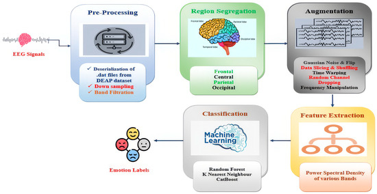
Figure 1.
The proposed FREQ-EER framework for emotion recognition and classification.
During the first step, that is, the preprocessing step, bandpass filtering is employed to separate critical EEG frequency bands like delta, theta, alpha, beta, and gamma, which are typically identified for conveying significant emotional information. Secondly, the EEG channels are then systematically divided into brain areas, such as the frontal, central, parietal, and occipital lobes. This brain-region-specific grouping allows the model to capture localized neural activity patterns that are closely associated with emotional processing. Next, to address the challenge of limited data and improve model generalization, we apply a set of frequency-based data augmentation techniques (as described in Section 3.5). These techniques bring realistic variations to the EEG signals without compromising their physiological correctness and thereby increase the size of the training set and decrease overfitting. Following augmentation, the DEAP dataset’s continuous emotional labels are binarized through median-based thresholding and separated into discrete emotional states like high or low arousal and valence according to the experimental conditions. During the feature extraction step, we use Welch’s power spectral density estimation to calculate band power features from each EEG signal. These features are able to sum up the frequency-domain properties of brain activity and are highly diagnostic of emotional states. For the final classification stage, an ensemble learning strategy with soft voting, aggregating the strengths of three lightweight yet efficient machine learning models: random forest (RF), CatBoost (CB), and K-Nearest Neighbors (KNN), are employed. This ensemble method enhances accuracy and stability while providing model interpretability and lower computational complexity. To make sure the framework is reliable and applicable to other scenarios, we verify it through a 10-fold cross-validation approach that measures how the model works over various divisions of data. To evaluate the emotional states of various participants, researchers normally bank on well-established psychological models that provide structured frameworks for interpreting affective responses. One such widely adopted model is Russell’s circumplex model of affect (1983) [20], which has also been employed in this study. As illustrated in Figure 2, this model represents emotions in a two-dimensional space.
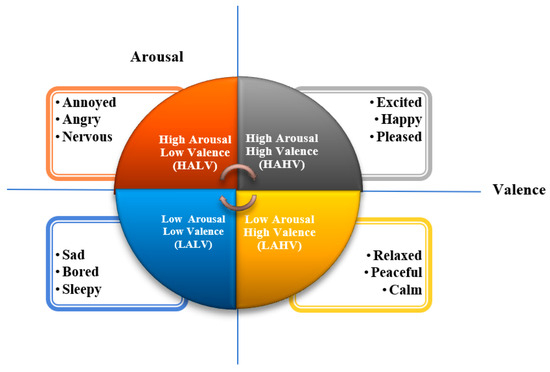
Figure 2.
Russell’s 2D Valence–Arousal emotion model.
The horizontal axis shows Valence, which describes how unpleasant or pleasant an emotion feels. The vertical axis shows Arousal, which describes how calm or excited a person feels, ranging from low energy (like being relaxed) to high energy (like being excited or nervous). This two-dimensional Russell’s model facilitates a finer classification of emotions; for instance, happiness is defined by High Arousal and High Valence, while sadness maps to Low Arousal and Low Valence. The simplicity and interpretability of the model make it especially well-adapted for EEG-based emotion recognition research, where intricate physiological signals need to be translated into understandable emotional states.
3.2. Dataset Description
A number of benchmark datasets such as the DEAP [21], MEG-based multimodal database for decoding affective physiological responses (DECAF-MEG) [22], database for emotional analysis in music and electroencephalogram recordings (DREAMER) [23], SJTU emotion EEG dataset (SEED) [24], and database for an emotion recognition system based on EEG signals and various computer games (GAMEEMO) [25], have been proposed by researchers. Among them, the DEAP dataset, one of the most popularly used datasets for emotion recognition based on EEG signals, has been used to evaluate our model. This dataset consists of EEG signals collected from 32 participants, as each watched one-minute-long excerpts of music videos. The participants rated each video on a scale of 1–9 in terms of four labels, viz. Arousal, Valence, Dominance, and Liking, among which Valence (defines the positive or negative nature of the emotion) and Arousal (defines the level of intensity of the emotion) were chosen for our study. Further, the median values of the two labels were calculated, such that values above 5 were considered high while below 5 were placed into low categories. These categories were then combined to form the four quadrants of the Russell’s emotion wheel, presented in Figure 2, High Arousal High Valence (HAHV), High Arousal Low Valence (HALV), Low Arousal Low Valence (LALV), and Low Arousal High Valence (LAHV). The labeling into the four quadrants was performed to map a larger set of emotions. Table 1 provides a more detailed description of the DEAP dataset.

Table 1.
Description of the DEAP dataset [21].
3.3. Band Filtration
As we are well aware, the human brain generates electrical signals that can be easily measured with the help of EEG (electroencephalography). These signals characteristically fall within a frequency range of 0 to more than 100 Hz, with amplitudes lying between 20 and 100 microvolts (µV). Therefore, based on their frequency, EEG signals are typically classified into numerous bands, namely, Delta (0.1–4 Hz), Theta (4–8 Hz), Alpha (8–13 Hz), Beta (13–30 Hz), and Gamma (30–100 Hz). Each of these bands is further associated with definite mental as well as emotional states. For instance, alpha waves are associated with calmness and relaxation, beta waves to alertness and concentration, theta waves to deep relaxation or meditation, and gamma waves to advanced thinking and memory processing. Therefore, to better understand the relationship that exists amongst the brain activity and emotional states, the DEAP dataset is employed, which comprise EEG recordings of individuals as they experience different emotions. In this paper, for experimental purposes, the EEG signals are separated into four key frequency bands: theta, alpha, beta, and gamma. This aids us to investigate and further understand how each type of brainwave participates and contributes to various emotional and cognitive responses. Such an approach not only helps in the investigation of human emotions but also in understanding brain functions and detecting neurological disorders.
3.4. Brain Region Segregation and Selection
EEG signals are obtained by the placement of electrodes on human scalp, capturing the brain’s electrical activity. The accuracy and reliability of the emotion classification system is largely dependent upon the placement of electrodes and the signal capture hardware utilized. A number of different methods have been developed for electrode placement towards signal acquisition; among them the International 10–20 system is the most widely used and accepted framework for clinical purpose and research work. The system, represented in Figure 3a, sets out specific electrode placements in the scalp ensuring consistent interelectrode spacing and labeling based on scalp positions. The different labels established are frontal (F), central (C), parietal (P), occipital (O), and temporal (T), with intermediate positions (e.g., FC (Frontal Central), CP (Central Parietal), PO (Parietal Occipital)) and midline points (e.g., Fz, Cz, Pz). Left-side electrodes have odd numbers, while right-side electrodes have even numbers. The second visual reference, Figure 3b, illustrates the segregation of the human brain based on various lobes, with each lobe corresponding to specific cognitive and emotional functions. This mapping from the electrode placement to brain lobe helps researchers form a strategic selection of electrodes based on the emotional relevance of brain regions, which in turn helps reduce the number of electrodes. This knowledge helped us select specific electrodes such as the frontal lobe for emotional regulation (F3, F4, F7, F8), the temporal lobe for emotional memory (T3, T4, T5, T6), and the occipital lobe for visual emotion processing (O1, O2), instead of using all 32 channels of the DEAP dataset. Furthermore, a detailed analysis of brain–band emotion relationships was carried out where different frequency bands correlated with specific brain lobes or specific sets of emotions were investigated.
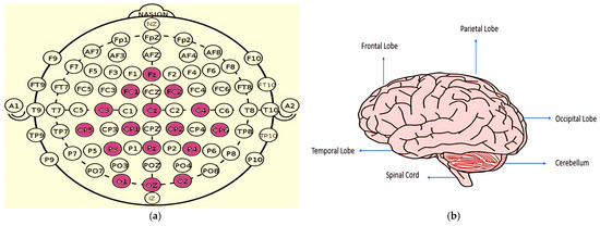
Figure 3.
(a) 10–20 Electrode Placement System (b) Different regions of Human Brain.
3.5. Data Augmentation Techniques Used and Their Mathematical Formulations
A major issue in EEG emotion identification is the requirement of a large dataset for efficient model training. In studies in medical research, where most data variables are sensitive information, collecting enough training data for model performance improvement is more challenging [26]. Therefore, creating synthetic data is a viable way to increase sample size, in turn enhancing data generalization, reducing the risk of overfitting and thereby ensuring better recognition of underlying patterns. The generation of new samples from existing ones through various kinds of transformations in order to increase accuracy measures of the classifier is known as data augmentation. Exposing the classifier to more variable representations of its training samples makes the model more invariant and robust to transformations of the type that it is likely to encounter when attempting to generalize unseen samples [27]. Although data augmentation is a well-established method in computer vision and despite a number of recent studies, data augmentation is still under explored for EEG data. Hence, we experimented with five different types of augmentation techniques, namely Gaussian noise addition and flip, data slicing and shuffling, time warping, random channel dropping, and frequency manipulation, to find the most effective one for EEG-based studies. The different augmentation techniques considered are discussed as being under the following:
Gaussian Noise Addition and Flip: The inability to remove the noise inherently present in brain signals motivates the introduction of the Gaussian noise augmentation, which mimics this feature and promotes robustness to EEG acquisition noise [6]. Gaussian noise addition introduces slight random perturbations to the signal, helping the model generalize to unseen data. This is mathematically expressed as
where is the original signal; is the added Gaussian noise, having a zero mean and a variance of .
Flipping, in the context of EEG signal augmentation, refers to reversing the time axis of the signal. Considering that the orientation of the time axis has no effect on the signal’s power spectral density (PSD), it can be hypothesized that flipping the time axis preserves most of the information while generating a new input. It can be expressed as
where is the time index of the signal, is the flipped signal at index , is the length of the signal, and represents the original signal at index .
Data Slicing and Shuffling: This technique involves slicing the EEG signal into smaller time windows and shuffling the data to prevent overfitting. Slicing is the time series data augmentation equivalent to cropping for image data augmentation. The general concept behind slicing is that the data is augmented by slicing time steps off the ends of the pattern [28]. It can be expressed as
where is the number of segments and is a function that randomly permutes these segments.
Time Warping: Time warping is the act of perturbing a pattern in the temporal dimension. This can be performed using a smooth warping path [29] or through a randomly located fixed window [30]. This method randomly stretches and compresses sub-segments to form the augmented samples. It randomly selects sub-segments to stretch and compress, with the recombination method to reassemble all the sub-segments and construct the warping-augmented signal with the same dimension as the origin EEG signal. Given an original signal the warped signal is defined as
where is a scaling factor ( > 1 compresses the signal, < 1 stretches it).
Random Channel Dropping: This technique of data augmentation simulates signal loss. If X is a multichannel signal with C channels, dropping can be represented as
where ∈ ℝ2 is a binary mask vector (zeros for dropped channels and ones for active channels).
Frequency Manipulation: For many EEG classification tasks, it is believed a substantial part of the information lies in the frequency domain of the recording [31,32]. This technique alters specific frequency components of the signal. For a given band power feature at frequency f, the manipulated power is defined as
where is a scaling factor ( > 1 amplifies the power, < 1 attenuates it).
3.6. Feature Extraction-Band Power Estimation Using Welch Method
Band power is an important feature, used in a number of the literature work for EEG signal analysis. It represents the amount of energy within each frequency range that is closely associated with different cognitive and emotional states. In our study, band power was extracted from the theta (4–8 Hz), alpha (8–13 Hz), beta (13–30 Hz), and gamma (30–45 Hz) bands utilizing Welch’s method of power spectral density (PSD) estimation. The Welch method is a crucial method in signal processing; power spectrum estimation (PSE) shows how an energy of signal is distributed among its many frequency components. By using a smoothing function to lessen unpredictability, the Welch method, an enhanced version of the traditional periodogram, improves the estimation of power spectral density [33]. The Welch method offers significant advantages over other power spectral density (PSD) estimation methods, particularly in terms of noise reduction, improved frequency resolution, and robustness to noise [34].
In this method, the EEG signal is initially divided into multiple overlapping segments. Each of these segments is windowed using the Hann function. Following the usage of the function, fast Fourier transform (FFT) is computed to estimate the power spectrum of each segment. These individual values are then averaged to obtain the final PSD estimate [33]. This averaging helps in significantly reducing the variance of the spectral estimate while preserving the frequency resolution. The mathematical representation of the PSD, denoted by , is
where denotes the k-the segment of the signal, is the window function applied to each segment, and denotes the total number of segments.
Further, in our study, the band power features within each frequency band (alpha, beta, theta, and gamma) [35] using the above equation. This is achieved by selecting all frequency bins such that each [] where and define the lower and upper limits of each individual band. The band power is then obtained by integrating the PSD over the given frequency range. In order to achieve a higher accuracy in numerical integration, Simpson’s rule is employed.
The value represented by Equation (8) represents the absolute band power present in each of the specified frequency band where denotes the average power density estimate of the signal.
3.7. Classification Using the Ensemble Model
The ensemble classification method plays a crucial role in enhancing the robustness, generalization, and interpretability of the model in our study. An ensemble model works by combining the predictive capability of multiple individual classifiers and mitigates the weaknesses of each. To build our ensemble model we experimented with a wide range of traditional classifiers including support vector machine (SVM), decision tree (DT), naïve Bayes (NB), multi-layer perceptron (MLP), AdaBoost (AB), XGBoost (XG), LightGBM (LGBM), Gaussian process classifier (GPC), and perceptron (PER), in addition to KNN, random forest (RF), and CatBoost (CB). At this stage of the study, no augmentation technique was used. The individual classifiers performance’s were evaluated across all four emotional labels (HAHV, HALV, LALV, and LAHV) and the highest accuracy achieved using specific band–region combinations was recorded as shown in Table 2. Results achieved showed that KNN, RF, and CB were among the top performing classifiers across various band–region combinations. For instance, KNN achieved 88.60%, RF up to 87.62%, and CB up to 88.60% accuracy in the LAHV band, outperforming the others. Similar patterns were observed in the other labels making these three suitable candidates for our base learners. Furthermore, when combined using a soft voting scheme, their ensemble performance (Table 2) further improved over the individual classifiers, motivating the use of the ensemble for further analysis. Importantly, while RF took 187.33 s, CB 269.82 s, and KNN 171.28 s to run individually, the ensemble required only 290.34 s. Similarly, the memory and CPU usage for RF was 6574.02 MB and 2.20%, respectively, 6498.39 MB and 7.30% for CB, and 6471.07 MB and 2.50% for KNN, while the ensemble needed only 6595.67 MB and 2.50%, demonstrating that the integrated model remained lightweight while improving overall performance.
Table 2.
Accuracy measures using various classifiers and the ensemble of top three classifiers.
The main feature of FREQ-EER that distinguishes it from the prior studies is the following:
- The comprehensive band–region-specific analysis. While most of the exiting works have considered all of the EEG channels uniformly or have not performed an explicit analysis of the influence of EEG frequency bands across brain regions, our model introduces the breakdown of EEG signals into four different frequency bands—theta, beta, alpha, and gamma and four brain regions—frontal, central, parietal, and occipital.
- To build a generalized model, a range of augmentation techniques, namely Gaussian noise addition, time flipping, time warping, data slicing and shuffling, random channel dropping, and frequency manipulation, were used. These techniques assisted in increasing the variability of the dataset while preserving the characteristics of the signal. Band power features [36,37] were extracted using Welch’s method [33,34], which is a spectral estimation technique that computes the power spectral density [35] of EEG signals.
- Feature extraction was performed from each of the distinguished frequency bands, which was followed by a detailed investigation into how specific oscillatory activity in specific brain regions correlated with distinct emotional states. For instance, analysis revealed that gamma activity strongly correlated with High Arousal positive emotions This band–region combination classification performance was evaluated across the four emotional classes: HAHV, HALV, LAL, and LAHV.
- The three classifiers—RF, CB, and KNN—were trained independently on the same set of features and emotion labels. Table 3 highlights the different parameters considered in our work for various classifiers employed in the ensemble model.
Table 3. Descriptions of the different parameters for various classifiers.
Further, each classifier generates probabilistic predictions against all four emotion classes, HAHV, HALV, LALV, and LAHV, and the final prediction is derived through soft voting, where the average of the predicted class probabilities is computed. Standard evaluation metrics such as accuracy and ROC AUC were used to compare the performance of individual models versus the ensemble, while demonstrating the superiority of each approach. The algorithm for the proposed FREQ-EER ensemble emotion classification is illustrated as Algorithm 1.
| Algorithm 1: FREQ-EER Ensemble Emotion Classification | |
| Input: | Raw EEG Data (DEAP dataset), Original Emotion Labels (Valence, Arousal) |
| Output: | Predicted Emotion Classes (HAHV, HALV, LAHV, LALV) |
| Step 1: | Begin |
| Step 2: | Load EEG data and emotion labels |
| EEG_data ← load_DEAP_dataset () | |
| Labels ← extract_valence_arousal_labels () | |
| Step 3: | Preprocess EEG data |
| Apply bandpass filtering (alpha, beta, theta, gamma) | |
| Down sample EEG_data to reduce complexity | |
| Step 4: | Apply data augmentation |
| For each signal in EEG_data: | |
| Augment with Gaussian noise using Equation (1) | |
| Perform time flipping using Equation (2) | |
| Perform data slicing and shuffling using Equation (3) | |
| Apply time warping using Equation (4) | |
| Perform channel dropping using Equation (5) | |
| Conduct frequency manipulation using Equation (6) | |
| Step 5: | Segment EEG channels by brain regions: |
| Frontal, central, parietal, occipital | |
| Step 6: | Extract Band Power Features |
| For each frequency band (theta, alpha, beta, gamma): | |
| Compute power using Welch’s Method using Equations (7) and (8) | |
| Step 7: | Relabel emotion labels |
| For each sample in Labels: | |
| If Valence ≥ 5 and Arousal ≥ 5 → HAHV | |
| If Valence < 5 and Arousal ≥ 5 → HALV | |
| If Valence ≥ 5 and Arousal < 5 → LAHV | |
| If Valence < 5 and Arousal < 5 → LALV | |
| Step 8: | Normalize features |
| features ← normalize(features) | |
| Step 9: | Split data (subject-independent) |
| (X_train, y_train), (X_test, y_test) ← train_test_split (features, rela beled_labels) | |
| Step 10: | Train base classifiers |
| model_RF ← train random forest on (X_train, y_train) | |
| model_CB ← train CatBoost on (X_train, y_train) | |
| model_KNN ← train KNN on (X_train, y_train) | |
| Step 11: | Perform predictions |
| probs_RF ← model_RF. predict_proba(X_test) | |
| probs_CB ← model_CB. predict_proba(X_test) | |
| probs_KNN ← model_KNN.predict_proba(X_test) | |
| Step 12: | Soft voting ensemble |
| avg_probs ← (probs_RF + probs_CB + probs_KNN)/3 | |
| y_pred ← argmax(avg_probs) | |
| Step 13: | Evaluate model |
| Calculate accuracy, ROC AUC | |
| Step 14: | End |
4. Results and Discussion
This section highlights the results obtained using the proposed FREQ-EER framework using the methodologies and datasets outlined in Section 3. To evaluate the performance of the different models under study, we focus on these two metrics first: accuracy as well as the receiver operating characteristic (ROC) curve. Accuracy is calculated as the number of correctly predicted instances divided by the total number of predictions made by the model. Although it measures model performance with a single metric, in the case of class imbalance, it does not provide insight regarding the effectiveness of the model. In addition, we consider using the ROC curve, which provides a summary measure of performance across all possible classification thresholds. The ROC curve captures the tradeoff between sensitivity and specificity defined by plotting the true positive rate (Sensitivity) and the false positive rate (1—Specificity). A key descriptive measure calculated from the ROC curve is the area under the curve (AUC). A model’s ability to differentiate instances from different classes is indicated by the AUC value, where higher values support a stronger discriminatory ability. Thus, a model approaching AUC 1.0 is regarded as effective, whereas 0.5 indicates no better than random performance.
4.1. Gaussian Noise Addition and Flip
HAHV and HALV Class: The HAHV class achieves its highest accuracy in the beta band (occipital region, 88.60%) (Table 4) with an ROC of 0.82 (Figure 4a) supporting the role of the beta band in visual processing and increased cognitive engagement during positive High Arousal states. On the other hand, HALV performs best in the alpha band (parietal region, 87.30%) (Table 4), suggesting the crucial role of alpha bands in the parietal region during High Arousal negative emotions such as anger and frustration. The HALV class displays a lower ROC AUC of 0.73% (Figure 4b).
Table 4.
Accuracy of HAHV and HALV classifications across various brain regions using different EEG bands and the Gaussian noise addition and flip method.
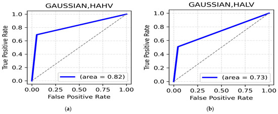
Figure 4.
(a). ROC curve for HAHV; (b). ROC Curve for HALV.
LALV and LAHV Class: The highest accuracy for the LALV class is observed in the theta band (central region, 85.67%) (Table 5) with an ROC of 0.7 (Figure 5a), indicating Low Arousal negative emotions are represented in theta activity. Theta (occipital, 84.04%) (Table 3) and alpha, parietal regions, also show strong performances, supporting the role of slower rhythms in negative emotion processing. For the LAHV class, the highest accuracy is observed in theta bands (occipital, 89.90%) (Table 5) with an ROC of 0.82 (Figure 5b). Similarly central and occipital alpha, 88.60% and 88.27%, support the association between alpha activity and relaxed wakeful states.
Table 5.
Accuracy of LALV and LAHV classification across various brain regions using different EEG bands and the Gaussian noise addition and flip method.
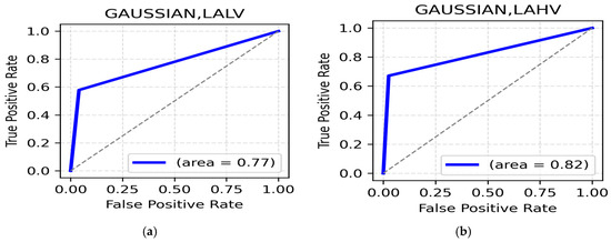
Figure 5.
(a). ROC curve for LALV; (b). ROC curve for LAHV.
4.2. Data Slicing and Shuffling
HAHV and HALV class: Classification results for the HAHV class using data slicing and shuffling as an augmentation technique reinforce the role of alpha activity in cognitive processing and emotion regulation, since the highest accuracy is shown in the alpha band (parietal region, 85.78%) (Table 6) with a ROC AUC of 0.78 (Figure 6a). Meanwhile, the highest accuracy in the HALV class is in the alpha band (central, 86.27%) (Table 6), ROC AUC of 0.72 (Figure 6b).
Table 6.
Accuracy of HAHV and HALV classification across various brain regions using different EEG bands and the data slicing and shuffling method.
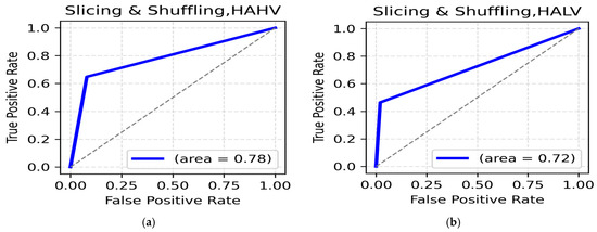
Figure 6.
(a). ROC curve for HAHV; (b). ROC curve for HALV.
LALV AND LAHV Class: While using the data slicing and shuffling method, the highest accuracy for the LALV class was seen in the alpha band (central, 88.73%) (Table 7). The ROC AUC was reported to be 0.84 (Figure 7a). The highest accuracy for LAHV, was again seen in the alpha band (central, 90.20%) with a ROC AUC value of 0.81 (Figure 7b), suggesting the dominance of the alpha band in distinguishing Low Arousal positive emotions.
Table 7.
Accuracy of LALV and LAHV classification across various brain regions using different EEG bands and the data slicing and shuffling method.
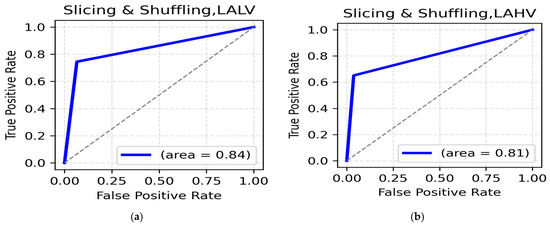
Figure 7.
(a). ROC curve for LALV; (b). ROC curve for LAHV.
4.3. Time Warping
HAHV and HALV Class: The highest accuracy for HAHV is in the gamma band (frontal, 76.96%) (Table 8), while central region in theta (76.47%) (Table 8) also shows strong performance. The ROC AUC was reported to be 0.62 (Figure 8a). For the HALV class, the theta band (occipital, 76.96%) (Table 8) and alpha band (frontal and central, 76.47%) (Table 7) gave superior performances. The ROC AUC value for the HALV class was recorded at 0.64 (Figure 8b).
Table 8.
Accuracy of HAHV and HALV classification across various brain regions using different EEG bands and the time warping method.
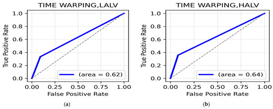
Figure 8.
(a). ROC curve for HAHV; (b). ROC curve for HALV.
LALV and LAHV Class: The highest accuracy for the LALV class is in the theta band (frontal, 77.45%) (Table 9). Next to theta, alpha (parietal, 76.47%) (Table 9) proved to be quite efficient in distinguishing Low Arousal negative emotions. As displayed in Figure 9a, the ROC AUC value for this class was 0.62. For the LAHV class, the highest accuracy is observed in the theta (frontal, central, parietal, 81.37%) (Table 9) and alpha band (central, 81.37%) (Table 9). The ROC AUC value is 0.67 (Figure 9b).
Table 9.
Accuracy of LALV and LAHV classification across various brain regions using different EEG bands and the time warping method.
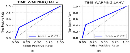
Figure 9.
(a). ROC curve for LALV; (b). ROC curve for LAHV.
4.4. Random Channel Dropping
HAHV and HALV Class: Random channel dropping performs relatively better for both the HAHV and HALV classes. The highest accuracy in the HAHV class is reported by the gamma band (occipital, 84.31%) (Table 10), while the frontal regions also show strong classification performance with accuracies of ~83%. The highest accuracy is in beta (parietal, 85.78%) (Table 10) for the HALV class, indicating that beta rhythms in the parietal region contribute to distinguishing High Arousal negative emotions. The ROC AUC values for HAHV and HALV are 0.74 and 0.69, respectively (Figure 10a,b).
Table 10.
Accuracy of HAHV and HALV classification across various brain regions using different EEG bands and random channel dropping.
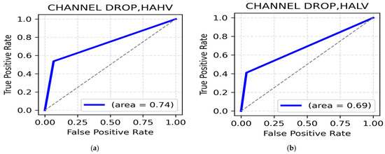
Figure 10.
(a). ROC curve for HAHV; (b). ROC curve for HALV.
LALV and LAHV class: The highest classification accuracy for the LALV class, using random channel dropping as the augmentation technique was recorded at 86.27% in the beta band, frontal region (Table 11) with a ROC AUC value of 0.73 (Figure 11a). On the other hand, the theta band in the central region reported the highest accuracy of 87.75 (Table 11), thereby supporting the importance of theta rhythms in distinguishing Low Arousal positive emotions. The ROC AUC in this class was 0.76 (Figure 11b). Additionally, frontal gamma (86.76%) and occipital alpha (86.27%) suggest gamma and alpha associations for cognitive stability and attentional balance in Low Arousal positive emotions such as calmness and contentment.
Table 11.
Accuracy of LALV and LAHV classification across various brain regions using different EEG bands and the random channel dropping method.
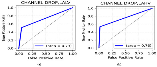
Figure 11.
(a). ROC curve for LALV; (b). ROC curve for LAHV.
4.5. Frequency Manipulation
HAHV and HALV class: The frequency manipulation augmentation technique yields the highest classification accuracy. In the HAHV class, the gamma band (parietal, 92.65%) (Table 12) recorded the highest value, with a ROC AUC value of 0.86 (Figure 12a). Meanwhile, for the HALV class of emotions such as anger and anxiety, the beta band in the central region and gamma in the parietal region provided a satisfactory accuracy of 91.67% (Table 12), reflecting increased cognitive processing and emotional stress, with an impressive ROC AUC value of 0.86 (Figure 12b).
Table 12.
Accuracy of HAHV and HALV classification across various brain regions using different EEG bands and the frequency manipulation method.
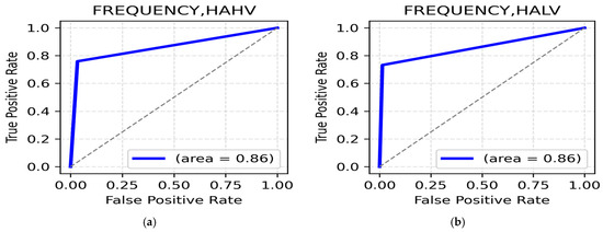
Figure 12.
(a). ROC curve for HAHV; (b). ROC curve for HALV.
LALV and LAHV Class: The highest accuracy for the LALV class was for the gamma band (parietal region, 95.59%) (Table 13), indicating high frequency oscillations in the parietal region while processing Low Arousal negative emotions with a ROC AUC value reaching up to 0.90 (Figure 13a). For the LAHV class, the highest accuracy was reported in the gamma band (occipital, 95.59%) (Table 13), highlighting the importance of occipital gamma rhythms in differentiating Low Arousal positive emotions. The ROC AUC value was 0.90 (Figure 13b).
Table 13.
Accuracy of LALV and LAHV classification across various brain regions using different EEG bands and the frequency manipulation method.

Figure 13.
(a). ROC curve for LALV; (b). ROC curve for LAHV.
Furthermore, we also explored the combined approach including all the augmentation techniques discussed previously (Section 4.6), namely Gaussian noise addition and flip, data slicing and shuffling, time warping, and random channel dropping, to evaluate its performance. However, the performance of the combined model was still lower than our proposed model FREQ-EER, which further demonstrated the reliability of our approach.
4.6. Combined Augmentation Techniques
HAHV and HALV class: In the HAHV class, the alpha band (central,88.44%) (Table 14) recorded the highest value, with a ROC AUC value of 0.81 (Figure 14a). Meanwhile, for the HALV class of emotions such as anger and anxiety, the alpha band in the occipital region provided a satisfactory accuracy of 89.90% (Table 14), with a ROC AUC value of 0.81 (Figure 14b).
Table 14.
Accuracy of HAHV and HALV classification across various brain regions using different EEG bands and combined augmentation techniques.
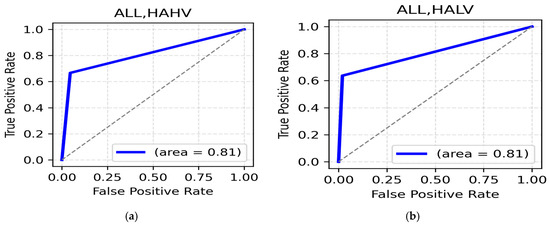
Figure 14.
(a). ROC curve for HAHV; (b). ROC curve for HALV.
LALV and LAHV Class: The highest accuracy for the LALV class was for the alpha band (central region, 89.25%) (Table 15), with a ROC AUC value reaching up to 0.79 (Figure 15a). For the LAHV class, the highest accuracy was observed in the alpha band (occipital, 89.58%) (Table 15). The ROC AUC value was 0.83 (Figure 15b).
Table 15.
Accuracy of LALV and LAHV classification across various brain regions using different EEG bands and Combined Augmentation Techniques.
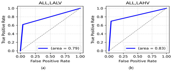
Figure 15.
(a). ROC curve for LALV; (b). ROC curve for LAHV.
Comparing the average results of various augmentation techniques (Table 16) suggests that manipulation is the most effective method, providing the highest accuracy across all classes, particularly in the gamma and beta bands within the parietal and occipital regions. Additionally, it required the least amount of processing time (583.93 sec). Along with superior accuracy and speed, it also relied on a minimum number of electrodes, with only five electrodes (parietal or occipital) for specific emotions such as HAHV, LALV, and LAHV and seven electrodes (central) for HALV emotions, making it an efficient model for the development of low-cost, real-time EEG-based emotion recognition systems. Following the frequency augmentation technique, the combination of all augmentation techniques provided a satisfactory performance across all states but required 2207.02 s, the highest among all techniques. Gaussian noise addition and flip also performed well, especially in occipital regions, suggesting their importance in HAHV and LAHV classification. Contrarily, time warping recorded the lowest classification accuracy, indicating the negative impact of temporal distortions on emotional features. The specific band–region analysis performed revealed parietal and occipital region significance for High Arousal emotions, while alpha and theta bands in the central and frontal regions and gamma in the parietal and occipital are best suited for identifying Low Arousal states. These findings of key EEG regions will enable the building of emotion detection devices with reduced electrodes, thereby simplifying the devices while maintaining the performance.
Table 16.
Comparing Accuracy of across various labels using different Augmentation techniques and reduced electrode count.
5. Model Evaluation on the SEED
Following the augmentation and classification experiments on the DEAP dataset, the SEED was selected as the next dataset to test for the discriminative ability of FREQ-EER across different datasets with different temporal, spectral, and emotional representations. While the DEAP provides a continuous emotional labeling framework based on Valence–Arousal, using 32 channels, SEED uses three discrete emotional labels: negative, neutral, and positive, recorded at a 200 Hz sampling frequency. It consists of 45 sessions from 15 participants, each containing 15 trials of recordings while the participants were presented with film clips as stimuli. The differences in emotional labels, experimental settings, and acquisition frequency made the SEED an ideal choice for cross corpus evaluation of the model originally developed using DEAP.
5.1. Gaussian Noise Addition and Flip
The Gaussian method achieved high classification accuracies across all classes (Table 17), with accuracies of 98% for the negative and neutral class and 100% for the positive class, providing an overall accuracy of 99%. ROC curves (Figure 16a) display all three classes achieving an AUC of 1.00, indicating perfect separability.
Table 17.
Classification accuracy of FREQ-EER on the SEED.
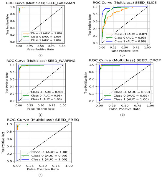
Figure 16.
ROC curve for the SEED using (a) Gaussian noise addition and flip; (b) data slicing and shuffling; (c) time warping; (d) random channel dropping; and (e) frequency manipulation.
5.2. Data Slicing and Shuffling
Data slicing and shuffling provided mixed results, with accuracies of 71% for negative emotion, 80% for neutral, and 91% for positive emotion, yielding an average value of 81% (Table 17). Figure 16b reflects AUC values of 0.88 for negative, 0.94 for neutral, and 0.99 for positive emotions. The reduced performance for the negative class suggests that slicing and shuffling may not be the optimal choice for EEG classification.
5.3. Time Warping
Time warping delivered a stronger classification performance with 92% for negative emotion, 93% for neutral, and 100% for positive emotion with an average accuracy of 95% as displayed in Table 17. Similarly, the ROC curves (Figure 16c) reflect AUC values of 0.99 for negative and neutral, and 1.00 for positive label.
5.4. Random Channel Dropping
With 94% for negative, 93% for neutral, and 99% accuracies for positive emotion, the random channel dropping augmentation technique provided an overall accuracy of 96%, indicated in Table 17. While the ROC curves show an AUC value of 0.99 (Figure 16d) for both negative and neutral, it was recorded to be 1.00 for the positive class. The results suggest that even when the channels are randomly dropped, the SEED contains enough information across EEG channels, enabling robust classification.
5.5. Frequency Manipulation
The frequency manipulation augmentation technique emerged as one of the most effective techniques with 97% for negative, 96% for neutral, and 99% for positive emotions, yielding an average accuracy of 97% (Table 17). The ROC curves (Figure 16e) display almost perfect separability with AUC values of 1.00 for negative and positive emotions and 0.99 for neutral. This augmentation technique is particularly effective because it is most closely associated with emotional processing, without changing the temporal information.
On comparing the SEED and DEAP dataset results, FREQ-EER emerges as the most consistent augmentation technique, providing high accuracies across all labels (97–99%) for the SEED’s three discrete emotion labels and DEAP’s continuous Valence–Arousal labels often exceeding 90% across all frequency bands and regions. This superior performance can be attributed to its direct target on emotion-relevant frequency bands (beta, theta, delta, alpha, and gamma), enhancing discriminative features without changing the signal. The robustness of the technique is reflected in the consistent ROC AUC scores of greater than 0.99 across both datasets, proving its strong class separability and generalization capability. FREQ-EER’s success in datasets with different sampling ratings, emotional labels, and experimental protocols makes it a promising choice for EEG-based emotion recognition applications.
6. Model Evaluation on the GAMEEMO Dataset
Following the classification and validation of the ensemble model on the DEAP and SEED, the GAMEEMO dataset which presents a unique dataset induced through gameplay was selected as another independent dataset. Instead of the usual videos or films, emotions in the GAMEEMO dataset were elicited while participants actively engaged in gaming tasks, resulting in dynamic and real emotional experiences. It consists of signals collected from 28 different subjects and 14 electrodes using the Emotiv EPOC headset. Compared with the SEED and DEAP, the reduced channel count limits spatial resolution in the GAMEEMO dataset, yet this dataset reflects the type of hardware and experimental settings relatable to real-world settings. The signals were recorded at a sampling frequency of 128 Hz and preprocessed using bandpass filters (0.5–45 Hz), along with artifact rejection, and segmentation. Participants were required to play four different computer games, each designed to elicit one of the different emotional states: boring, calm, horror, and funny. GAMEEMO presents a more realistic context compared with the controlled settings of the DEAP and SEED, and hence was an optimal choice for the cross-data validation.
6.1. Gaussian Noise Addition
Using Gaussian noise addition, the ensemble model achieved excellent results across the four classes (Table 18). Accuracies of 98% for bored, 100% for calm, 100% for horrified, and 98% for amused were achieved, leading to an overall accuracy of 98.9%. ROC curves (Figure 17a) further confirmed the efficiency of the model, with all four classes having an AUC value of 1.00, indicating perfect separability. These results reconfirm the earlier findings of Gaussian noise addition being one among the most robust augmentation methods to make the model more generalized across different type of datasets.
Table 18.
Classification accuracy of FREQ-EER on the GAMEEMO dataset.
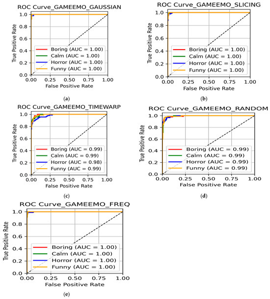
Figure 17.
ROC curve for GAMEEMO dataset using (a) Gaussian noise addition and flip; (b) data slicing and shuffling; (c) time warping; (d) random channel dropping; and (e) frequency manipulation.
6.2. Data Slicing and Shuffling
It was yet another augmentation technique that performed strongly on the GAMEEMO dataset with accuracies of 98% for boring, 99% for calm, 99% for horror, and 97% for funny and an overall accuracy of 98.03% (Table 18). ROC analysis (Figure 17b) yields an AUC value of 1.00 across the four emotion classes. Although it performed very well on GAMEEMO, slicing and shuffling led to reduced accuracy in the SEED, indicating that the augmentation technique was dataset-dependent and is highly effective only under certain experimental conditions.
6.3. Time Warping
Relative to other techniques, time warping delivered moderate classification performance on GAMEEMO wherein the accuracies reported were 89% for boring, 92% for calm, 94% for horror, and 92% for funny, leading to an overall accuracy of 91.2% (Table 18). ROC curves (Figure 17c) with AUC values ranging between 0.98 and 0.99 across the four classes demonstrate strong separability of the model.
6.4. Random Channel Dropping
Dropping channels randomly achieved good results, with accuracies of 93% for boring, 95% for calm, 94% for horror, and 92% for funny, giving an overall accuracy of 93.8% (Table 18). ROC curves (Figure 17d) represent perfect separability with AUC values of 0.99 across all classes. These results suggest that even with randomly dropped channels, sufficient discriminative features remain for effective classification.
6.5. Frequency Manipulation
Frequency manipulation emerged as one among the best-performing techniques on the GAMEEMO dataset. Accuracies achieved were 97% for boring, 100% for calm, 100% for horror, and 98% for funny, yielding an overall accuracy of 98.6% (Table 18). ROC curves (Figure 17e) showed an AUC of 1.00 for all four classes, indicating perfect separability. These results agree with the results achieved on the SEED and the DEAP dataset, indicating frequency-based features as the most robust augmentation strategy for emotion classification.
7. Comparison with Existing Work
Further, a comparative analysis between various state-of-the-art EEG-based emotion classification methods and our proposed model FREQ-EER, focusing on the datasets used, emotions classified, augmentation techniques employed, reported accuracies, and number of electrodes used, is presented in Table 19. GAN-based augmentation methods provide an average accuracy range of 94.87–97.14%, with Alidoost, Y., & Asl, B. M. (2025) [13] achieving 94.44% (HAHV), 96.55% (HALV), 98.19% (LALV), and 97.52% (LAHV) on DEAP, but requiring 18 channels. Similarly, Zhang, Z. et al. (2024) [16] achieved 96.33% (Valence) and 96.88% (Arousal) on the DEAP and 97.14% on the SEED while requiring up to 62 channels. In contrast, our proposed method, the frequency manipulation-based approach (FREQ-EER), achieves an accuracy range of 91–96%, providing comparable accuracies with state-of-the art models while offering significantly reduced electrode count possibility. For instance, it required only five channels for HAHV, LALV, and LAHV and seven channels for HALV, demonstrating high accuracy without depending on all 32 channels of the DEAP or highly dense 62 channels of the SEED. The validation of the model on the SEED and GAMEEMO further confirmed the robustness of the model.
Table 19.
Comparison of emotion classification accuracy: existing vs. proposed approach.
Furthermore, the novelty of our work is the detailed analysis of the association of different regions of the brain and frequency bands of the EEG signal. Such detailed analysis provides insights into how different regions of the brain are associated with different emotional states. Such an analysis is vital in the development of efficient BCIs, where precise and accurate emotion recognition is required.
8. Conclusions and Future Work
This study presents the effectiveness of the frequency-based ensemble method for emotion recognition, FREQ-EER, which can handle challenges such as the need for an extensive dataset and intensive resources and dependence on complex deep learning architectures. The benefits of employing traditional augmentation techniques such as Gaussian noise addition and frequency manipulation are evident particularly when applied to smaller datasets like the DEAP, while also maintaining strong generalization on larger and structurally different datasets like the SEED and GAMEEMO. Results suggest that frequency manipulation provided the highest classification accuracy across all classes of emotion, particularly in the gamma and beta bands within the parietal and occipital regions, indicating their importance in distinguishing different emotional states. Next to frequency manipulation, the Gaussian noise addition and flip was the most effective, especially in the occipital and parietal regions. The simpler augmentation methods and ML algorithms were able to enhance generalization while minimizing the risk of overfitting commonly seen when using the deep learning approaches. This line of action, i.e., specific band-to-brain-region analysis, not demonstrated in any previous work, not only reduces computational demands but also makes the model interpretable, offering a clear understanding of how specific frequency bands and brain regions relate to particular emotional states. The results of this study will lead to the development of more affordable EEG headsets without any compromise on performance, making real-time emotion monitoring systems more feasible for everyday use. There is no doubt that the proposed framework has demonstrated significant success in emotion recognition and classification. However, there remains considerable scope for further exploration and enhancement. Building on this foundation, the following research directions are outlined below, which may serve as a valuable guide for researchers:
- In the future, one can think of developing more sophisticated augmentation techniques to improve data diversity and enhance classification performance.
- The proposed FREQ-EER can be used on additional EEG datasets, such as DECAF-MEG and AMIGOS, to confirm the efficiency of the suggested model and assess generalization across various participants, sensors, and recording conditions.
- Attention mechanisms may be incorporated into machine learning models in the future, to enhance interpretability and highlight the most pertinent brain regions and frequency bands for emotion recognition.
- The FREQ-EER framework may be applied to real-world domains such as mental health monitoring, gaming, and adaptive interfaces to test its practical applicability.
- In the future, efforts can be made to optimize and deploy lightweight models on edge devices like mobile phones or wearables for real-time, on-device emotion recognition without cloud dependency.
Author Contributions
Conceptualization, D.T. and R.R.; methodology, D.T.; software, D.T.; validation, D.T. and R.R.; formal analysis, D.T. and R.R.; investigation, D.T.; resources, D.T.; data curation, D.T. and R.R.; writing—D.T. and R.R.; writing—review and editing, D.T. and R.R. All authors have read and agreed to the published version of the manuscript.
Funding
This research received no external funding.
Institutional Review Board Statement
This article does not contain any studies with human participants or animals performed by any of the authors.
Informed Consent Statement
Not applicable.
Data Availability Statement
The dataset for emotion analysis using physiological signals (DEAP), one of the most popularly used datasets for emotion recognition, was used for our study. To access the dataset, one needs to visit their official website at www.eecs.qmul.ac.uk/mmv/datasets/deap (accessed on 23 February 2022).
Acknowledgments
The authors would like to thank Sikkim University and Sikkim Institute of Science and Technology for their support.
Conflicts of Interest
The authors declare no conflict of interest.
References
- Alarcao, S.M.; Fonseca, M.J. Emotions recognition using EEG signals: A survey. IEEE Trans. Affect. Comput. 2017, 10, 374–393. [Google Scholar] [CrossRef]
- Oude Bos, D. EEG-based emotion recognition. Influ. Vis. Audit. Stimuli 2006, 56, 1–17. [Google Scholar]
- Liu, Y.; Sourina, O.; Nguyen, M.K. Real-Time EEG-Based Emotion Recognition and Its Applications. In Transactions on Computational Science XII. Lecture Notes in Computer Science; Tan, C.J.K., Sourin, A., Sourina, O., Eds.; Springer: Berlin/Heidelber, Germany, 2011; Volume 6670, pp. 256–277. [Google Scholar] [CrossRef]
- Alhalaseh, R.; Alasasfeh, S. Machine-learning-based emotion recognition system using EEG signals. Computers 2020, 9, 95. [Google Scholar] [CrossRef]
- Zheng, W.L.; Lu, B.L. Investigating critical frequency bands and channels for EEG-based emotion recognition with deep neural networks. IEEE Trans. Auton. Ment. Dev. 2015, 7, 162–175. [Google Scholar] [CrossRef]
- Wang, F.; Zhong, S.H.; Peng, J.; Jiang, J.; Liu, Y. Data augmentation for EEG-based emotion recognition with deep convolutional neural networks. In MultiMedia Modeling; Springer International Publishing: Bangkok, Thailand, 2018; Part II 24; pp. 82–93. [Google Scholar] [CrossRef]
- Acharjee, R.; Ahamed, S.R. EEG Data Augmentation Using Generative Adversarial Network for Improved Emotion Recognition. In Pattern Recognition; Springer Nature: Cham, Switzerland, 2025; pp. 238–252. [Google Scholar] [CrossRef]
- Luo, Y.; Zhu, L.Z.; Wan, Z.Y.; Lu, B.L. Data augmentation for enhancing EEG-based emotion recognition with deep generative models. J. Neural Eng. 2020, 17, 056021. [Google Scholar] [CrossRef] [PubMed]
- Adhikari, S.; Choudhury, N.; Bhattacharya, S.; Deb, N.; Das, D.; Ghosh, R.; Ghaderpour, E. Analysis of frequency domain features for the classification of evoked emotions using EEG signals. Exp. Brain Res. 2025, 243, 65. [Google Scholar] [CrossRef] [PubMed]
- Prakash, A.; Poulose, A. Electroencephalogram-Based Emotion Recognition: A Comparative Analysis of Supervised Machine Learning Algorithms. Data Sci. Manag. 2025, 8, 342–360. [Google Scholar] [CrossRef]
- Li, M.; Xu, H.; Liu, X.; Lu, S. Emotion recognition from multichannel EEG signals using K-nearest neighbor classification. Technol. Health Care 2018, 26, 509–519. [Google Scholar] [CrossRef]
- Kumar, A.; Kumar, A. Human emotion recognition using Machine learning techniques based on the physiological signal. Biomed. Signal Process. Control 2025, 100, 107039. [Google Scholar] [CrossRef]
- Alidoost, Y.; Asl, B.M. Entropy-based Emotion Recognition Using EEG Signals. IEEE Access 2025, 13, 51242–51254. [Google Scholar] [CrossRef]
- Cruz-Vazquez, J.A.; Montiel-Pérez, J.Y.; Romero-Herrera, R.; Rubio-Espino, E. Emotion recognition from EEG signals using advanced transformations and deep learning. Mathematics 2025, 13, 254. [Google Scholar] [CrossRef]
- Qiao, W.; Sun, L.; Wu, J.; Wang, P.; Li, J.; Zhao, M. EEG emotion recognition model based on attention and gan. IEEE Access 2024, 12, 32308–32319. [Google Scholar] [CrossRef]
- Zhang, Z.; Zhong, S.; Liu, Y. Beyond Mimicking Under-Represented Emotions: Deep Data Augmentation with Emotional Subspace Constraints for EEG-Based Emotion Recognition. In Proceedings of the AAAI Conference on Artificial Intelligence, Vancouver, BC, Canada, 20–27 February 2024. [Google Scholar] [CrossRef]
- Du, X.; Wang, X.; Zhu, L.; Ding, X.; Lv, Y.; Qiu, S.; Liu, Q. Electroencephalographic signal data augmentation based on improved generative adversarial network. Brain Sci. 2024, 14, 367. [Google Scholar] [CrossRef]
- Liao, C.; Zhao, S.; Wang, X.; Zhang, J.; Liao, Y.; Wu, X. EEG Data Augmentation Method Based on the Gaussian Mixture Model. Mathematics 2025, 13, 729. [Google Scholar] [CrossRef]
- Szczakowska, P.; Wosiak, A. Improving Automatic Recognition of Emotional States Using EEG Data Augmentation Techniques. In Proceedings of the Procedia Computer Science, Athens, Greece, 6–8 September 2023. [Google Scholar] [CrossRef]
- Russell, J.A.; Ridgeway, D. Dimensions underlying children’s emotion concepts. Dev. Psychol. 1983, 19, 795. [Google Scholar] [CrossRef]
- Koelstra, S.; Muhl, C.; Soleymani, M.; Lee, J.S.; Yazdani, A.; Ebrahimi, T.; Patras, I. Deap: A database for emotion analysis; using physiological signals. IEEE Trans. Affect. Comput. 2011, 3, 18–31. [Google Scholar] [CrossRef]
- Abadi, M.K.; Subramanian, R.; Kia, S.M.; Avesani, P.; Patras, I.; Sebe, N. DECAF: MEG-based multimodal database for decoding affective physiological responses. IEEE Trans. Affect. Comput. 2015, 6, 209–222. [Google Scholar] [CrossRef]
- Katsigiannis, S.; Ramzan, N. DREAMER: A database for emotion recognition through EEG and ECG signals from wireless low-cost off-the-shelf devices. IEEE J. Biomed. Health Inform. 2017, 22, 98–107. [Google Scholar] [CrossRef] [PubMed]
- Zheng, W.L.; Zhu, J.Y.; Lu, B.L. Identifying stable patterns over time for emotion recognition from EEG. IEEE Trans. Affect. Comput. 2017, 10, 417–429. [Google Scholar] [CrossRef]
- Alakus, T.B.; Gonen, M.; Turkoglu, I. Database for an emotion recognition system based on EEG signals and various computer games–GAMEEMO. Biomed. Signal Process. Control 2020, 60, 101951. [Google Scholar] [CrossRef]
- Rommel, C.; Paillard, J.; Moreau, T.; Gramfort, A. Data augmentation for learning predictive models on EEG: A systematic comparison. J. Neural Eng. 2022, 19, 066020. [Google Scholar] [CrossRef] [PubMed]
- Lashgari, E.; Liang, D.; Maoz, U. Data augmentation for deep-learning-based electroencephalography. J. Neurosci. Methods 2020, 346, 108885. [Google Scholar] [CrossRef] [PubMed]
- Iwana, B.K.; Uchida, S. An empirical survey of data augmentation for time series classification with neural networks. PLoS ONE 2021, 16, e0254841. [Google Scholar] [CrossRef]
- Um, T.T.; Pfister, F.M.; Pichler, D.; Endo, S.; Lang, M.; Hirche, S.; Kulić, D. Data augmentation of wearable sensor data for parkinson’s disease monitoring using convolutional neural networks. In Proceedings of the 19th ACM international Conference On Multimodal Interaction, Glasgow, UK, 13–17 November 2017. [Google Scholar]
- Le Guennec, A.; Malinowski, S.; Tavenard, R. Data augmentation for time series classification using convolutional neural networks. In Proceedings of the ECML/PKDD Workshop on Advanced Analytics and Learning on Temporal Data, Riva Del Garda, Italy, 19 September 2016. [Google Scholar]
- Zhu, Z.; Wang, X.; Xu, Y.; Chen, W.; Zheng, J.; Chen, S.; Chen, H. An emotion recognition method based on frequency-domain features of PPG. Front. Physiol. 2025, 16, 1486763. [Google Scholar] [CrossRef]
- Pillalamarri, R.; Shanmugam, U. A review on EEG-based multimodal learning for emotion recognition. Artif. Intell. Rev. 2025, 58, 131. [Google Scholar] [CrossRef]
- Özçoban, M.A.; Tan, O. Electroencephalographic markers in Major Depressive Disorder: Insights from absolute, relative power, and asymmetry analyses. Front. Psychiatry 2025, 15, 1480228. [Google Scholar] [CrossRef]
- Ikizler, N.; Ekim, G. Investigating the effects of Gaussian noise on epileptic seizure detection: The role of spectral flatness, bandwidth, and entropy. Eng. Sci. Technol. Int. J. 2025, 64, 102005. [Google Scholar] [CrossRef]
- Wang, Z.; Wang, Y. Emotion recognition based on multimodal physiological electrical signals. Front. Neurosci. 2025, 19, 1512799. [Google Scholar] [CrossRef]
- Garg, S.; Patro, R.K.; Behera, S.; Tigga, N.P.; Pandey, R. An overlapping sliding window and combined features based emotion recognition system for EEG signals. Appl. Comput. Inform. 2021, 21, 114–130. [Google Scholar] [CrossRef]
- Yan, F.; Guo, Z.; Iliyasu, A.M.; Hirota, K. Multi-branch convolutional neural network with cross-attention mechanism for emotion recognition. Sci. Rep. 2025, 15, 3976. [Google Scholar] [CrossRef]
Disclaimer/Publisher’s Note: The statements, opinions and data contained in all publications are solely those of the individual author(s) and contributor(s) and not of MDPI and/or the editor(s). MDPI and/or the editor(s) disclaim responsibility for any injury to people or property resulting from any ideas, methods, instructions or products referred to in the content. |
© 2025 by the authors. Licensee MDPI, Basel, Switzerland. This article is an open access article distributed under the terms and conditions of the Creative Commons Attribution (CC BY) license (https://creativecommons.org/licenses/by/4.0/).