1. Introduction
Channel estimation plays a pivotal role in wireless communication systems, facilitating accurate signal reception amidst the challenges posed by various types of noise. Reliable estimation of the channel enables more efficient data transmission by compensating for distortions caused by the communication environment [
1,
2,
3,
4]. The task becomes particularly challenging when the channel is influenced by non-Gaussian noise models, such as Bernoulli–Gaussian (BG) noise [
5]. This type of noise introduces intermittent and sparse impulses that can severely degrade the performance of traditional channel estimation techniques. In most conventional approaches, such as those assuming additive white Gaussian noise (AWGN), linear regression-based estimators have been widely used due to their simplicity and effectiveness in estimating the channel coefficients. However, when the noise deviates from the Gaussian assumption, such as in scenarios with impulsive noise, these methods often fail to provide optimal performance [
6,
7].
The BG noise model, which combines a sparse noise process with Gaussian perturbations, is a more realistic representation for various wireless environments. It includes urban and industrial settings where bursty interference is common. Several real-world datasets and measurement campaigns have demonstrated the presence of impulsive noise that follows a BG distribution, particularly in vehicular and cognitive radio networks [
8]. Studies like [
9] also show that power-line noise consists of both Gaussian background noise and impulsive components, which can be modeled accurately using a BG distribution. Moreover, it has been shown that wireless channels often exhibit heavy-tailed noise characteristics beyond Gaussian assumptions, making BG and even Cauchy-based noise models highly relevant for practical deployment [
10,
11].
While least squares (LS) and linear minimum mean square error (LMMSE) estimators remain widely adopted for channel estimation under Gaussian noise, they fail to maintain accuracy in the presence of impulsive, heavy-tailed interference [
12,
13,
14]. Robust regression approaches, such as M-estimators and expectation–maximization (EM) algorithms, can partially address impulsive effects, but they typically involve high computational burden and lack closed-form tractability in non-Gaussian settings. In contrast, our work introduces a regression framework that explicitly incorporates the BG distribution, leveraging the log-sum inequality (LSI) to derive a tractable negative log-likelihood bound and a gradient descent-based estimator. This enables robustness to impulsive noise while preserving interpretability and computational efficiency. Unlike deep learning-based approaches that demand large datasets and high training complexity, the proposed framework provides a lightweight alternative suitable for real-time deployment in wireless systems.
This paper proposes a novel approach to channel estimation tailored for scenarios characterized by BG noise. We explore the limitations of conventional methods and propose an enhanced linear regression approach that incorporates the characteristics of Bernoulli–Gaussian noise to improve the estimation accuracy [
15,
16,
17]. Additionally, we compare the performance of this method with advanced techniques, such as the LSI-based estimation, which is designed to handle sparse noise distributions. Leveraging the principles of linear regression, our method aims to accurately estimate the channel response, even in the presence of significant noise distortion [
18,
19]. The proposed technique begins by modeling the received signal as a linear combination of the transmitted symbols convolved with channel impulse response with added noise, which is BG in nature. We then formulate the channel estimation problem as a linear regression task, where the objective is to learn the parameters of the channel response matrix from the received signal samples. Other regression-based machine learning and deep learning models comprising neural networks have been used in several research articles for channel estimation [
16,
20,
21,
22,
23,
24].
Furthermore, with the rapid evolution of wireless technologies towards 5G, 6G, and beyond, the role of accurate channel estimation has become even more critical. Emerging paradigms such as massive multiple-input multiple-output (MIMO), reconfigurable intelligent surface (RIS), integrated sensing and communication (ISAC), and millimeter-wave (mmWave) transmission demand highly reliable estimation methods to ensure low-latency and high-throughput performance [
1,
2]. In such advanced architectures, non-Gaussian noise, particularly impulsive BG interference, is becoming increasingly common due to spectrum sharing, dense deployment, and hybrid heterogeneous networks [
5,
9,
25].
Recent studies on deep learning (DL)-based channel estimation [
21,
22] and unfolded iterative solvers [
19,
26] have demonstrated improved robustness to non-linear channel conditions. But these approaches often require large training datasets, suffer from high computational complexity, and lack interpretability [
27]. In contrast, the proposed regression-based framework retains computational efficiency while explicitly modeling impulsive BG noise characteristics, striking an optimal balance between robustness and tractability.
The main contributions of this paper are summarized as follows:
We employ a robust regression framework to address the challenges posed by BG noise [
28] which combines discrete and continuous characteristics. By incorporating suitable regularization techniques and optimization algorithms, our method effectively mitigates the impact of noise on the channel estimation process [
29].
We derive a closed-form approximation of the maximum-likelihood estimator and design an iterative gradient descent approach optimized for sparse noise distributions.
We evaluate the performance of the proposed approach through extensive simulations and compare it with existing methods under non-Gaussian noise conditions. The results demonstrate the superior accuracy and robustness of our technique, particularly in scenarios with high noise levels and sparse channel impulse responses.
We provide insights into the applicability of the proposed framework for emerging wireless paradigms, including RIS-aided systems, massive MIMO, and ISAC-driven 6G communications. Overall, the proposed channel estimation method offers a promising solution for wireless communication systems operating in environments prone to Bernoulli–Gaussian noise, thus enhancing reliability and performance in practical deployment scenarios.
2. System Model
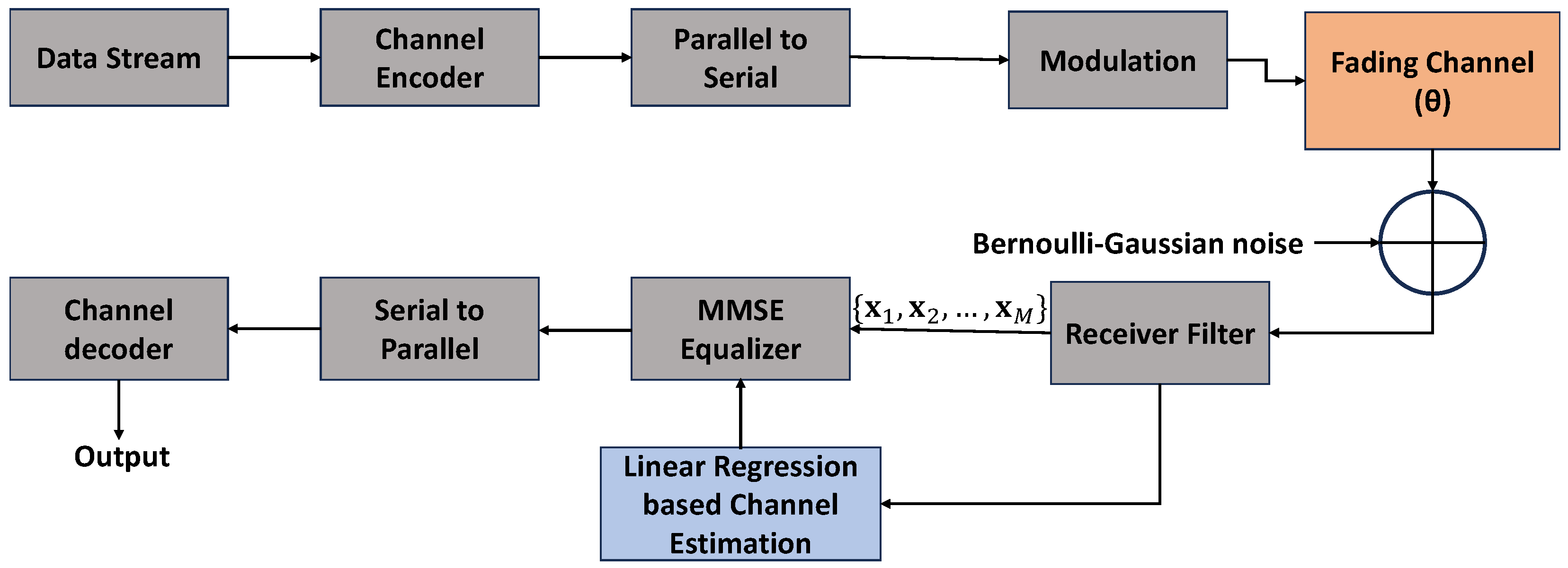
We consider an end-to-end multiple-input single-output communication system with additive non-Gaussian noise, as shown in
Figure 1. In this system, the goal is to estimate the wireless channel by using linear regression techniques while dealing with additive Bernoulli–Gaussian noise. In emerging wireless systems, noise environments deviate significantly from Gaussian assumptions due to impulsive interference caused by device switching, electromagnetic emissions, and spectrum-sharing mechanisms. BG noise captures these dynamics effectively by combining a Gaussian background with sparse impulses, making it particularly suitable for power-line communication (PLC), RIS-assisted mmWave, and dense Internet of Things (IoT) deployment [
5,
9].
We consider a data stream represented by a real-valued unitary matrix given by
, where
is the transpose operator and each column
is transmitted through an
N antenna system. As a result, we receive baseband signal
sampled at
M observations, considering each instant of the time frame individually. The main focus of this work is to use parametric models, which entail choosing a function with parameters and figuring out the best parameter values
to describe the provided data. In general, the functional dependence of
on
is defined as:
where
is complex BG noise. Here,
indicates the unknown channel-related parameters.
We assume that the
i-th sample of an independent variable,
, is supplied and that a dependent variable,
, is the noisy observation that is produced in parallel with the input. Although the framework is presented for a SISO setting for clarity, it can be extended to multi-antenna scenarios (MISO/MIMO) by generalizing the regression formulation across multiple transmit and/or receive antennas. Such extensions are reserved for future work. We use the signal-to-noise ratio (SNR) to express how strong a signal is in relation to noise levels; it is generalized as
where
is the expectation operator. In order to evaluate the accuracy of the predictive models, mean square error (MSE) is used as a performance metric in machine learning [
30]. It is the averaged mean over channel realization, including number of observations and training samples:
where
is the true value and
is its estimate.
2.1. Approximate Maximum-Likelihood Estimator Using Log-Sum Inequality
Let us formulate our problem from (
1) by stating the probability density function (PDF) of the Bernoulli–Gaussian noise as [
31]
Here,
, where
is the hyperparameter that gives the prior probability of the noise originating with variance
. The Bernoulli–Gaussian (BG) noise model assumes that each noise sample
is drawn from a mixture of two Gaussian distributions: with probability
,
is Gaussian with variance
(background noise), and with probability
,
is Gaussian with variance
(impulsive noise). Thus,
or
explicitly represents the impulse probability in the noise model. It represents the likelihood that a noise sample originates from the impulsive component. A useful measure of impulsive severity is the variance ratio,
which quantifies the relative strength of the impulsive noise with respect to the background noise. Larger values of
r correspond to more dominant impulsive components, while smaller values approach the Gaussian background case. Robust performance, therefore, requires the estimator to maintain stable accuracy across a range of
r and
values. By denoting the Bernoulli–Gaussian distribution by BG and substituting (
1) in (
4), we get
where
can be expressed by replacing
with
in (
4). Let us now move to parameter estimation in the following manner:
The goal of maximum-likelihood analysis is to maximize the likelihood function of the received data samples, considering the channel coefficients. The maximum-likelihood estimator (MLE) can be defined using the following equation:
It is evident that maximizing the log-likelihood function is equivalent to minimizing the negative log-likelihood function. In order to minimize the obtained negative log-likelihood function, we need to use the gradient descent method. Hence, we take negative log-likelihood of the PDF as follows:
It is instructive to observe that in the special case where and , the mixture distribution in (8) reduces to the Gaussian case. In this scenario, minimizing the negative log-likelihood is equivalent to minimizing , which corresponds exactly to the ordinary least squares (OLS) criterion. This connection highlights that the log-sum inequality (LSI) provides a generalized framework, which reduces to OLS under purely Gaussian assumptions.
Furthermore, to avoid ambiguity, we explicitly note that and denote the variance terms of the two Gaussian components, and and are the corresponding mixture weights satisfying . The expansion shows explicitly how the LSI provides a tractable upper bound on the negative log-likelihood. The scaling terms and are preserved throughout, which ensures that the derivation maintains consistency with the original probabilistic model.
Using the LSI
, where
, we have
Considering the equi-probability of occurrence of noise with variance
, we take the value of
for
:
By substituting (
11) into (
10), we get
We observe that the right-hand side of (
12) matches that of (
9). From the LSI, we can write (
9) as
Further, (
13) can be written as
In terms of square distance between
and
, we can write (
14) as
where
k is a relative constant. By computing the partial derivative of
with respect to
, we get
The expression for
derived under the LSI can be further simplified to a sub-optimal, closed form from (
17) as
We aim to iteratively refine the estimate by utilizing the gradient of the least squares error (LSE) between the received signal and the estimated channel response until the error is minimized. Consequently, we iterate the suggested iterative gradient descent algorithm until the computed error falls below a predetermined threshold . The variable denotes either the step size or the learning rate. Additionally, a residual threshold indicates the convergence point for the estimated channel coefficients, determining when to stop further iteration.
2.2. Proposed Maximum-Likelihood Estimator (Numerical Optimization)
To perform channel estimation using the gradient descent method and linear regression, we first need to define the problem and establish the objective function. Given the PDF for the BG noise model in (
4), we denote the
i-th antenna’s received signal by
and transmitted signal by
.
Our aim is to perform channel estimation for BG noise (impulsive); by substituting the PDF
in (
4) into the negative log-likelihood function, we get
To obtain the gradient of
in (
19), we differentiate each term with respect to
. Because (
19) contains a logarithm of a sum, we apply the chain rule. The resulting expression is shown in (
20), and detailed intermediate steps are provided in
Appendix A for clarity.
Further, we can update the parameter vector
iteratively using the gradient descent algorithm:
where
denotes the parameter vector at the
k-th iteration,
is the learning rate, and
is the gradient of
evaluated at
. Similar to Algorithm 1 we use the gradient descent method to update
until the algorithm converges.
| Algorithm 1 Iterative gradient descent algorithm. |
| Require: ▹ Channel to be estimated - 1:
Initialize - 2:
Calculate initial error - 3:
- 4:
repeat - 5:
▹ Step Updation - 6:
Calculate error - 7:
until
▹ Convergence
|
3. Methodology
In order to evaluate the proposed channel estimation framework under BG noise, we performed extensive Monte Carlo simulations. Each experiment consists of transmitting a sequence of pilot symbols through a wireless channel with additive BG noise. The following parameters were considered for the simulations (
Table 1):
This setup (
Table 1) enables a fair comparison between different channel estimation methods for identical noise environments and fading conditions. The MSE between the estimated channel coefficients and the true channel parameters was used as the primary performance metric.
LSI-based approximation is employed to handle the Bernoulli–Gaussian distribution, which consists of a mixture of Gaussian components with different variances. By applying the LSI, the negative log-likelihood function can be bounded and simplified, enabling tractable optimization.
The gradient descent algorithm is then applied to iteratively minimize the resulting loss function. Compared with closed-form MLE, gradient descent provides
Lower computational complexity in high-dimensional settings;
Robustness to impulsive noise samples;
Flexibility in adapting to varying noise variances.
Recently, machine learning and DL methods have been applied to channel estimation, showing promising results under complex fading and non-linear channel conditions [
21,
22,
27]. However, these methods typically suffer from three limitations:
Requirement of large labeled training datasets;
High computational complexity during both training and inference;
Lack of interpretability, which restricts practical deployment.
In contrast, the proposed regression-based framework explicitly models the impulsive characteristics of BG noise while maintaining computational efficiency and interpretability. This ensures robustness in non-Gaussian noise environments without relying on data-intensive training procedures.
The least squares (LS) estimator is obtained by minimizing the quadratic loss function
which is optimal only under Gaussian noise assumptions [
32]. The proposed estimator, BG-MLE, minimizes the negative log-likelihood of the Bernoulli–Gaussian mixture model.
where
and
denote the background and impulsive probabilities, respectively. Since the BG likelihood is non-convex, we employ an EM/IRLS approach in which the weights
and
act as sample-wise responsibilities, leading to iterative weighted least squares updates.
4. Results and Discussion
In this section, we illustrate the impact of Bernoulli–Gaussian noise on channel estimation for a single-antenna wireless communication system under Rayleigh fading.
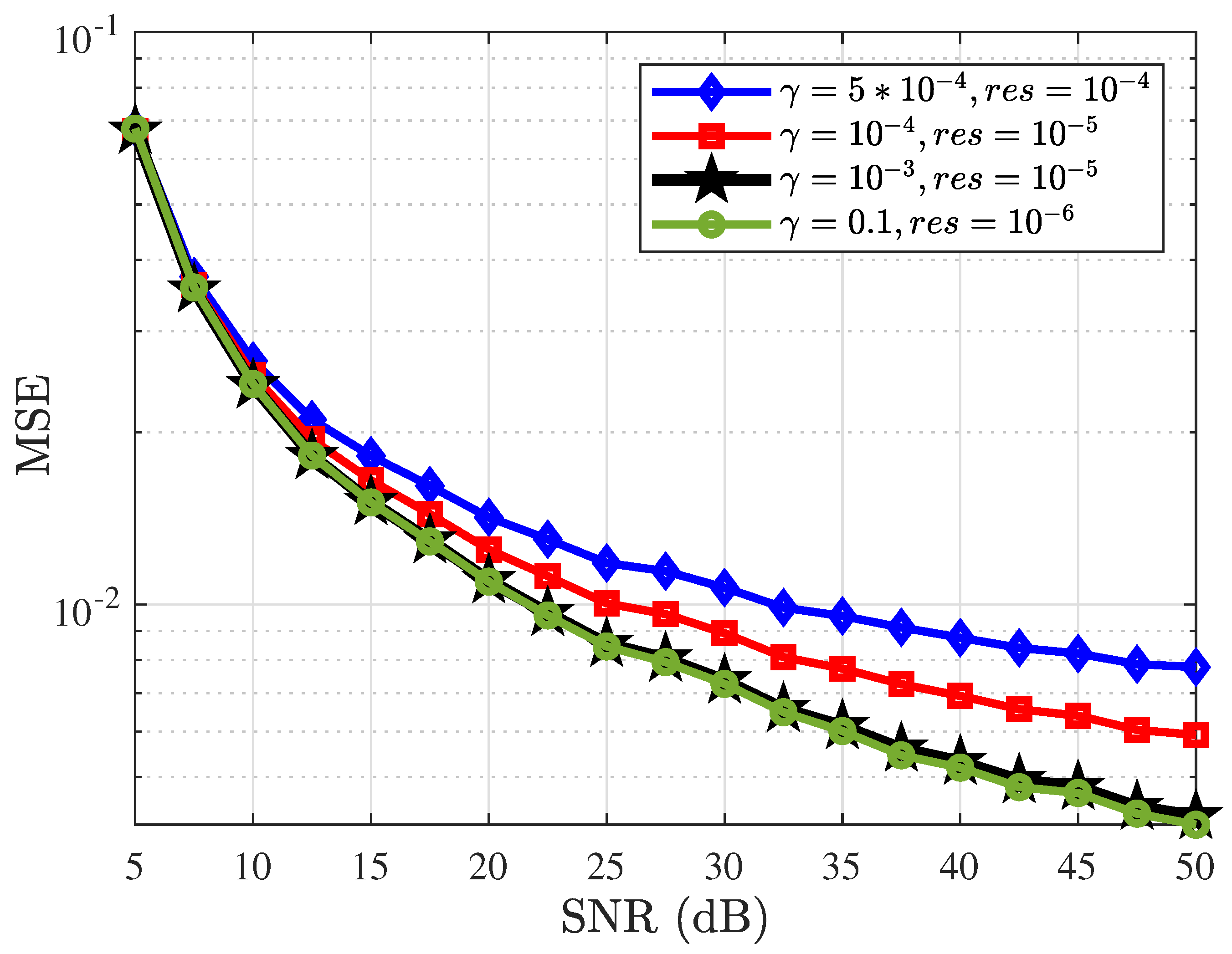
Figure 2 illustrates the relationship between the MSE and the SNR for four different parameter settings of the gradient descent algorithm in the context of Bernoulli–Gaussian noise using (
20) for
and
(as in Algorithm 1). As the SNR increases, the MSE decreases, indicating improved estimation accuracy at higher SNR levels. The curve corresponding to
and
demonstrates a relatively unstable and high MSE across the entire SNR range, suggesting that this parameter setting fails to provide a good balance between convergence speed and stability. The curve for
and
suggests moderate performance. The parameter setting
and
indicates high accuracy but potentially slower convergence. The parameter setting
and
results in significantly lower MSE values. This indicates that a smaller step size can lead to poor estimation accuracy and instability. The choice of step size
and residual threshold (
) critically affects the convergence behavior of the gradient descent algorithm. A large step size (e.g.,
) leads to oscillations and instability, yielding higher MSE across the SNR range. Conversely, a very small step size (e.g.,
) results in more stable convergence but at the cost of slower adaptation. The residual threshold
governs the stopping condition: loose thresholds may terminate prematurely, while overly strict values increase computational effort without significant accuracy gains. Hence, optimal performance requires balancing
and
, as reflected in the curve corresponding to
and
. Although
confidence intervals were also computed for these results, they are not plotted in
Figure 2 in order to maintain clarity of the comparison of step size versus residual threshold. The intervals confirm that the trends observed are statistically reliable.
Figure 3 illustrates the performance of MSE versus SNR for Gaussian noise and Bernoulli–Gaussian noise with two different sets of variance. In order to use the proposed estimator given in (
20) for Gaussian noise, we ignore the Bernoulli term by setting its probability of impulses to zero. The curve corresponding to a variance of
consistently shows a higher MSE compared with the curve with a variance of
across the entire SNR range. This indicates that Gaussian noise with a smaller variance yields better (lower MSE) at higher SNR values. The MSE for Gaussian noise follows a predictable pattern. Similarly, the MSE for Bernoulli–Gaussian noise decreases with the increase in the SNR but at a rate different from that of Gaussian noise. The curves for Bernoulli–Gaussian noise with variances of
and
show a higher MSE than those with variances of
and
at higher SNR values, indicating better performance for higher variance. This figure highlights the impact of Bernoulli–Gaussian noise on MSE performance, showing how the Bernoulli-distributed impulses affect the overall error compared with Gaussian noise.
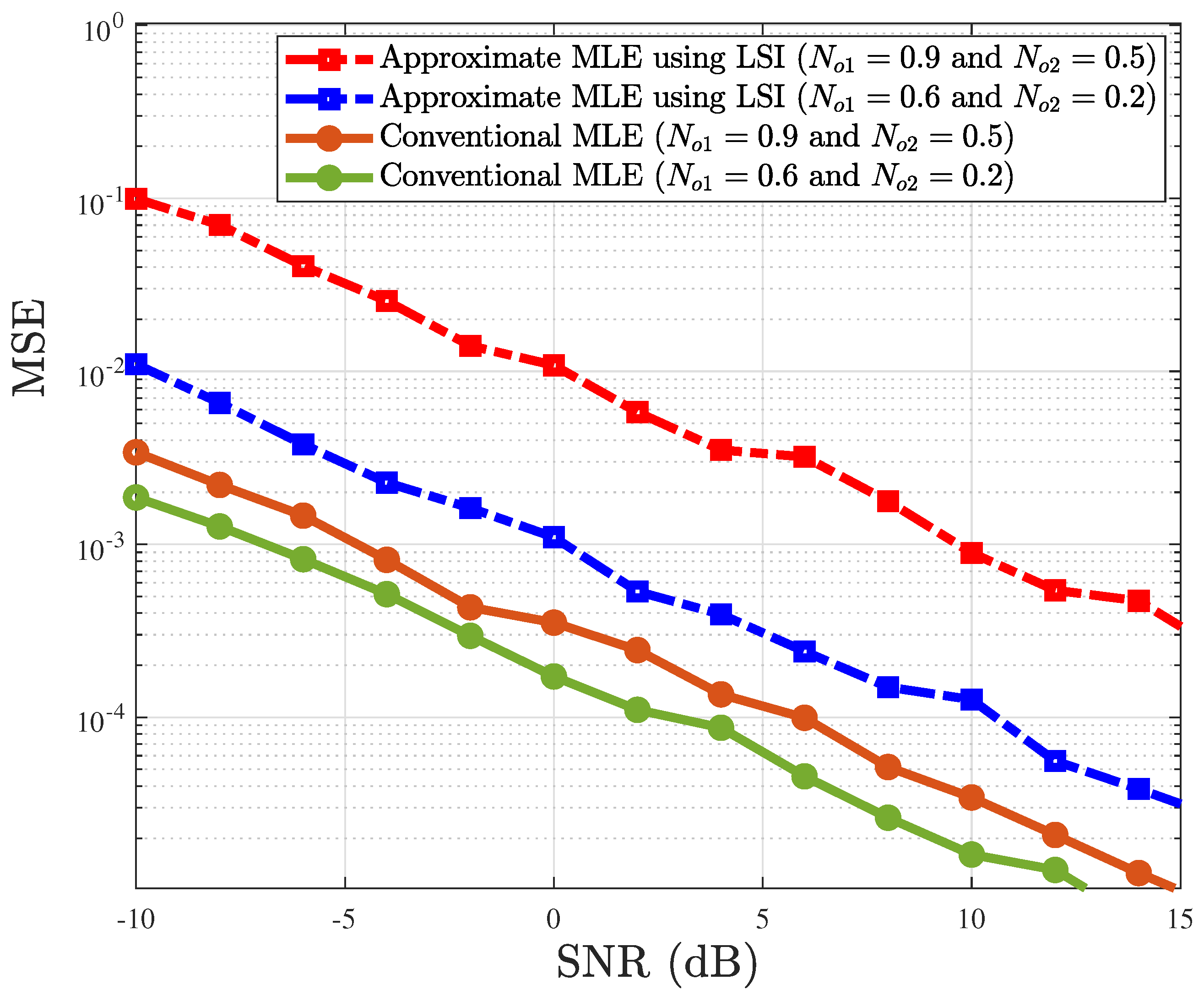
Figure 4 illustrates the performance of two channel estimation methods, approximate MLE using the LSI and the proposed MLE using the iterative gradient descent method by seeking derivatives from (
17) and (
20) for Bernoulli–Gaussian noise, for two sets of noise variances. The MSE is plotted against the SNR for each estimation technique. For both variance sets
and
, the proposed MLE consistently outperforms the LSI method across the entire range of SNR values. Notably, the MSE for the proposed MLE decreases more rapidly with the increase in the SNR, particularly for negative SNR values, demonstrating better robustness under low-SNR conditions. This aligns with the expectation that the proposed MLE method offers more reliable channel estimation across all data points. In contrast, the approximate MLE using LSI curves shows a higher MSE at low SNR values, indicating a lower convergence rate as the noise becomes more pronounced. However, with the SNR
dB, the performance of both estimators begins to converge, though the proposed MLE still maintains a lower MSE. This suggests that while LSI methods might be suitable in higher-SNR regimes, they are less effective under noisier conditions, as evidenced by the flatter decay in MSE for lower SNR values. The results indicate that the proposed MLE can better adapt to varying noise conditions, making it a preferred choice for practical communication systems where maintaining accurate channel estimates across a wide range of SNR values is crucial.
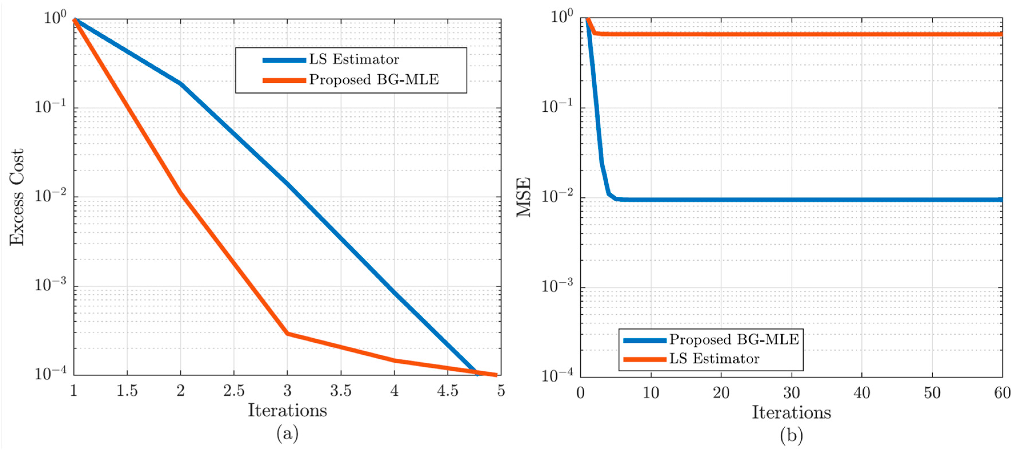
Convergence is analyzed both in terms of the excess negative log-likelihood and parameter MSE. The LS baseline optimizes the quadratic loss function, while BG-MLE optimizes the Bernoulli–Gaussian log-likelihood through iterative reweighting.
Figure 5 provides a detailed convergence analysis of the proposed estimator, BG-MLE, in comparison with the LS baseline.
Figure 5a shows the normalized excess negative log-likelihood as a function of the iteration index. Although the LS method exhibits a steeper initial decline, this rapid cost reduction is deceptive, as it does not guarantee accurate estimation under impulsive noise.
Figure 5b presents the normalized parameter MSE versus iterations. Here, the advantage of BG-MLE becomes evident: the proposed method reduces the estimation error by over two orders of magnitude within the first few iterations and remains stable thereafter. In contrast, the LS method stagnates at a high error level, failing to capture the channel parameters in the presence of Bernoulli–Gaussian noise. These results demonstrate that BG-MLE provides both reliable convergence and significantly superior estimation accuracy compared with the LS estimator, thereby validating its robustness under non-Gaussian noise conditions.
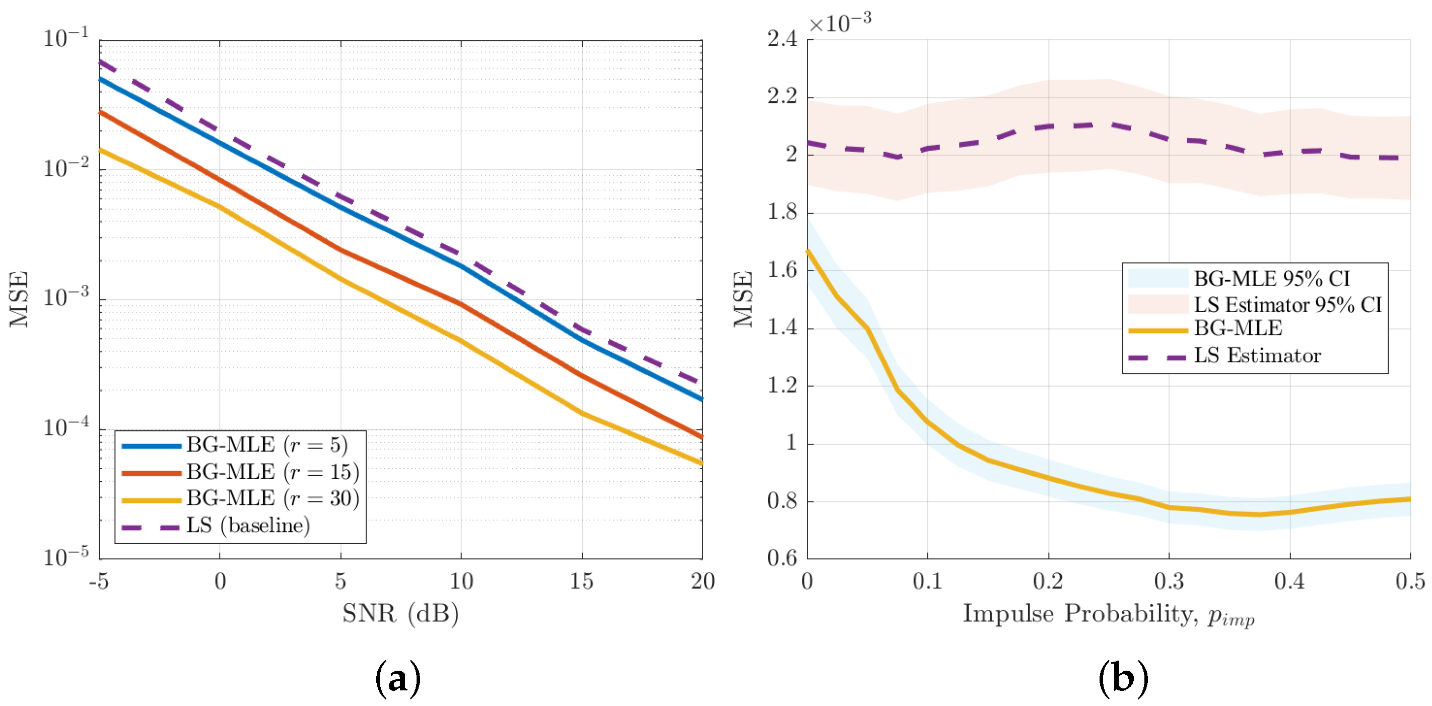
Figure 6 illustrates the robustness of the proposed estimator, BG-MLE, compared with the LS baseline under varying impulsive noise conditions.
Figure 6a plots the parameter MSE versus SNR for different impulsive variance ratios
at a fixed impulse probability
. As expected, all curves exhibit decreasing MSE with increasing SNR. However, BG-MLE achieves consistently lower error across the full SNR range and remains resilient as
r increases from 5 to 30. The LS baseline performs significantly worse, particularly in low- to mid-SNR regimes, highlighting its sensitivity to impulsive components. This demonstrates that BG-MLE maintains robust performance even as the impulsive-to-background noise power ratio varies.
Figure 6b presents the MSE versus impulse probability
at a fixed SNR of 10 dB and a variance ratio
. Here, BG-MLE sustains low MSE across the full range of
values, while the LS estimator shows consistently higher error and negligible adaptation to the impulsive component. The inclusion of 95% confidence intervals (shaded regions) confirms the statistical reliability of the trends observed. The results clearly demonstrate that BG-MLE not only achieves superior accuracy compared with LS, but also exhibits robustness against variations in both impulsive variance ratio and impulse probability, thereby addressing the reviewer’s concern regarding additional performance metrics beyond MSE versus SNR.
All reported results are obtained by averaging over 1000 independent Monte Carlo realizations to ensure statistical robustness. Results are averaged over 1000 independent runs with seed control (
rng(42) in MATLAB). For each performance curve,
confidence intervals were also computed. The error bars are explicitly shown in
Figure 5 and
Figure 6.
The computational complexity of the proposed estimator is significantly lower than that of LSI-based MLE approaches. The closed-form MLE requires matrix inversion, which has complexity , where N is the number of channel coefficients. In contrast, the proposed gradient descent estimator has complexity per iteration, where k is the number of iterations required for convergence. This makes the approach suitable for practical real-time implementations.
5. Conclusions
This work presented a robust channel estimation framework for wireless communication systems operating in BG noise environments. We developed an enhanced linear regression-based approach that explicitly incorporates the impulsive characteristics of BG noise and evaluated its performance against conventional Gaussian noise-based estimators and advanced maximum-likelihood methods. Through detailed analysis and extensive simulations, we demonstrated that the proposed framework achieves superior estimation accuracy and robustness, particularly in low-SNR regimes and scenarios characterized by sparse channel impulse responses. The results confirmed that the gradient descent-based estimator, derived from the log-sum inequality formulation, provides a favorable trade-off between accuracy and computational complexity. Specifically, the proposed approach achieves significant MSE improvements compared with Gaussian-based estimators while maintaining lower complexity than LSI-based closed-form MLE solutions. Owing to its computational efficiency and robustness under impulsive noise, the proposed framework is well-suited for real-time and resource-constrained wireless systems.
Beyond its methodological contributions, this study highlights the broader significance of BG noise modeling in modern communication environments. In applications such as power-line communications, vehicular ad hoc networks, and dense IoT deployment, impulsive interference frequently dominates, making Gaussian assumptions unrealistic. The proposed approach offers a practical solution that can be extended to advanced wireless paradigms, including massive MIMO, RIS, and mmWave transmission, and ISAC architectures envisioned for 6G systems. While the current work focuses on simulation-based evaluation, future research should extend this framework to experimental validation using real-world datasets. Moreover, hybrid approaches that combine machine learning models with regression-based estimation could further enhance adaptability under highly dynamic non-Gaussian environments. Another promising direction lies in extending the proposed methodology to multi-antenna and multi-user scenarios, as well as integrating it with adaptive pilot design strategies.
In summary, the proposed linear regression-based estimator provides an analytically tractable, computationally efficient, and practically relevant solution for robust channel estimation under Bernoulli–Gaussian noise. By bridging the gap between traditional statistical signal processing and emerging requirements of 5G/6G networks, this work contributes a valuable step towards reliable communication in non-Gaussian wireless environments. Future extensions of this work will explore hybrid regression-based methods and comparisons under Cauchy noise environments to further strengthen generalizability across diverse non-Gaussian noise models.
