3D Non-Uniform Fast Fourier Transform Program Optimization

Abstract

MRI (magnetic resonance imaging) technology aims to map the internal structure image of organisms. It is an important application scenario of Non-Uniform Fast Fourier Transform (NUFFT), which can help doctors quickly locate the lesion site of patients. However, in practical application, it has disadvantages such as large computation and difficulty in parallel. Under the architecture of multi-core shared memory, using block pretreatment, color block scheduling NUFFT convolution interpolation offers a parallel solution, and then using a static linked list solves the problem of large memory requirements after the parallel solution on the basis of multithreading to cycle through more source code versions. Then, manual vectorization, such as processing, using short vector components, further accelerates the process. Through a series of optimizations, the final Random, Radial, and Spiral dataset obtained an acceleration effect of 273.8×, 291.8× and 251.7×, respectively.

1. Introduction

Fast Fourier Transform (FFT) is an improved and fast algorithm based on Discrete Fourier Transform (DFT), which reduces the time complexity from O($N^2$) to O($nlogn$). It is widely used in the field of digital signal processing and has great significance [1]. The FFT algorithm is ubiquitous in everyday life and has brought great convenience to human society, making it one of the top ten algorithms of the 20th century [2]. However, the traditional FFT algorithm requires data samples to be distributed on a uniform grid, making it unable to handle non-uniform Cartesian network data, such as radar signal processing [3], CT reconstruction [4], MRI imaging [5], and computer tomography imaging [6].

To address the issue of non-uniformly sampled data, the Non-Uniform Fast Fourier Transform (NUFFT) has become the most effective solution, utilizing the fast properties of the FFT algorithm to avoid the unacceptable cost of computing the DFT. The primary task of NUFFT is to use convolution functions to interpolate the data on non-uniform grids to a uniformly distributed grid, which is an important step in data processing for the FFT algorithm. Experimental results have shown that in the entire calculation process of the NUFFT algorithm, the FFT is no longer the bottleneck of the program due to the use of the FFTW (Fastest Fourier Transform in the West) fast algorithm library. The real time-consuming part is the convolution interpolation operation.

The NUFFT algorithm was first applied in the field of astronomy. In 1975, Brouw [7] proposed the convolution interpolation (gridding) method, which implemented the fast Fourier transform for non-uniformly sampled data in polar coordinate grids. It was then applied in medical MRI imaging. In 1993, Dutt and Rokhlin proposed a fast algorithm based on the research of five formats of the Non-uniform Discrete Fourier Transform (NDFT) problem [8], which realized the conversion of non-uniform data to Cartesian coordinates, further expanding the application scope of the standard FFT algorithm. Since then, the NUFFT algorithm has received much attention. Research on NUFFT optimization includes the singular value decomposition method proposed by Caporale in 2007 [9], which mainly eliminates the commonly used window function weighting step. In 2008, Sorensen proposed the gpuNUFFT library based on GPU acceleration [10], greatly improving the computation speed of the FFT.

Reference [11] proposed a scalable scheduling block partitioning scheme to balance the load using blocks of different sizes, but the implementation is complex. Reference [12] optimized the TRON (Trajectory Optimized NUFFT) on the GPU based on the characteristics of the radial test set, which is highly targeted and cannot adapt to more complex datasets. In terms of memory, due to the large number of sampled data and high computational complexity of the NUFFT algorithm, Reference [13] introduced the mean square error formula to adjust the window size in interpolation, which has lower error but is computationally complex. In terms of data transformation, Reference [14] explores data parallelism by utilizing the geometric structure in data transformation and the processor-memory configuration in the target platform, with a focus on better utilizing the data in memory and improving cache hit rate during data transformation.

The background of this paper’s program optimization is 3D-MRI imaging (magnetic resonance imaging) [15]. Firstly, the signal information of the patient’s tissue site is collected, and then the Non-Uniform Fast Fourier Transform is used to reconstruct the layered images of the patient’s tissue site in the transverse, coronal, and sagittal planes at once. Non-Uniform Fast Fourier Transform can help doctors quickly obtain diagnostic information and has a wide range of applications in clinical medicine.

The main work and contributions of this paper are as follows:

1.

A feasible parallel optimization method is proposed for the convolution interpolation operation of the NUFFT algorithm;

2.

The proposed parallel optimization method is implemented on an Intel Xeon Platinum 9242 CPU machine;

3.

The optimization effects of different datasets are extracted through experimental data.

2. Target Platform and Program Features

2.1. Introduction to the Target Platform

The target platform for program optimization in this paper is an Intel server with four Intel Xeon Platinum 9242 CPUs, each with 24 physical cores, totaling 96 cores. Each core has a clock frequency of 2.3 GHz, and all cores share 191 GB of operating memory using the 100 GB Intel Omnipath interconnect network. From each core’s perspective, it supports Intel’s AVX512 vector instruction set, which can process 8 double-precision floating-point numbers at a time.

On the software side, the CentOS 8.0 operating system is used, and the program is compiled using ICC 19.1.1.217. In addition, the program calls the FFTW library for fast Fourier transform and the C++ Boost library to improve program performance.

2.2. Program Feature Analysis

2.2.1. Hotspot Analysis

Typical NUFFT-based iterative solvers use two NUFFT operators: Forward NUFFT (FWD) and Adjoint NUFFT (ADJ). The Forward NUFFT operates by applying a scaling function to the signal of interest, transforming the signal onto a uniformly spaced (i.e., Cartesian) spectral grid by means of an (oversampled) FFT, and then judiciously interpolating that signal onto the desired set of non-uniformly spaced (i.e., non-Cartesian) indices. The program uses two key operators for the NUFFT algorithm: The Forward NUFFT (FWD) and the Adjoint NUFFT (ADJ). The calculation process of the FWD operator can usually be divided into three steps:

1.

Applying a scaling function to the collected signal to weight the original data;

2.

Converting the signal to an equidistant signal and performing an oversampled FFT;

3.

Performing convolution interpolation on the result of oversampled FFT.

The ADJ operator can be seen as the inverse operation of the FWD operator. It first performs convolution interpolation of the non-uniformly spaced signal onto a uniform grid, then transforms the signal through FFT, and finally applies the scaling function to the obtained signal.

In the source program, there are timing functions for key functions and loops, and after the program completes its execution, the running times of each part are automatically output. Figure 1 shows the timing results for one iteration of the program. From the timing results, it can be seen that for both the ADJ operator and the FWD operator, the convolution interpolation part takes up the largest proportion of time, accounting for more than 85% of the total time. Therefore, the hotspot of the program is the convolution interpolation part of the data.

As shown in Figure 2, each convolution kernel consists of two parts. For a given sample point p, with coordinates (wx[p], wy[p], wz[p]), the first part computes interpolation kernel coefficients, winX, winY, and winZ, using table LUT look-up. It also computes x, y, and z coordinates of the neighbors in the convolution window, kx, ky, and kz. The second part performs actual convolution, where forward convolution accumulates weighted values from the Cartesian grid into the sample value and adjoint convolution spreads the sample value onto the Cartesian grid, as shown in Figure 2. In the actual program code of this paper, the pseudo code for the ADJ operator and FWD operator calculations are shown in Figure 2, which includes the common part 1 of the two operators, as well as the unique parts part2a and part2b. Preliminary analysis shows that the FWD operator can be directly parallelized, while the ADJ operator contains dependencies and cannot be directly parallelized.

2.2.2. Dataset

Due to the uncertain distribution of sampling data in the NUFFT algorithm, different sampling methods can have a significant impact on performance. Therefore, when optimizing the program, the load balancing problems caused by different datasets need to be considered. This program uses three representative datasets: Random, Radial, and Spiral, which fully demonstrate the performance of the NUFFT algorithm. As shown in Figure 3, the Random dataset has randomly distributed data points, the Radial dataset has a radial distribution with denser data points near the center, and the Spiral dataset has a spiral distribution.

3. Parallel Optimization Methods

3.1. OpenMP Multithreading Parallelism

The data update for the convolution interpolation part of the FWD operator is shown in Figure 4, where multiple data points are used to calculate and update the value of one point in each iteration of the loop. Since there are no dependencies, it can be directly parallelized.

The parallel method used in the final solution is OpenMP multithreading. By adding the “parallel for” directive to the outermost loop of the core loop, multiple threads are utilized to make use of the multi-core resources of the platform. From a load perspective, when multiple threads are enabled, the workload is evenly distributed, ensuring load balance. In this case, the simplest and most effective approach is used: using static scheduling provided by OpenMP, which strictly divides the load evenly and has no scheduling overhead. Another advantage is that static scheduling assigns physically adjacent data to the same thread as much as possible, ensuring data locality. In terms of the number of threads, considering the platform architecture and experimental results, 48 threads provide the best performance.

The data update for the convolution interpolation part of the ADJ operator within the loop is shown in Figure 5. Compared to the FWD operator, there are data dependencies caused by the protocol. The data points required for updating one point are distributed in different iterations of the loop, resulting in loop-carried dependencies. It cannot be directly parallelized and requires some data processing to achieve parallelism.

3.2. Block Pretreatment

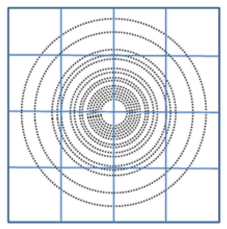
To address the issue mentioned in Section 3.1 and ensure that the dependencies in the loop can be correctly executed in parallel, the data are first block-pretreated. The source program has data distributed in a discrete structure in three-dimensional space. Figure 6 shows a one-dimensional cross-section of the three-dimensional data. The data are unevenly distributed throughout the entire three-dimensional space. By dividing the data into blocks, the data are independent within each block, and the points within each block are executed sequentially, which further exploits the parallelism between blocks.

After block pretreatment, it is necessary to determine how many points exist in each block and which points they are. The initial approach was to create an array for each block to store the points. However, due to the uneven distribution of points in space, it is not possible to determine the size of the array, so the array is defined as large as possible to ensure that the storage does not overflow. Through testing, it was found that this approach, although ensuring the correct execution of block data, introduces new problems:

1.

Excessive space occupation due to uneven data distribution.

2.

The cost of block pretreatment (is high) exceeds the core computational time after parallelization.

To address problem (1), a solution is to use a static linked list to store the data, so that all the data are stored in the linked list. Only one array of length equal to the number of data points in the dataset is defined in the structure, and an integer variable cursor is defined to indicate the successor element. This way, all elements share the entire data space, eliminating space waste and reducing memory access pressure. The pseudo code for the specific implementation is shown in the first part of Listing 1, including the definition and initialization of the linked list.

To address problem (2), the preprocessing of data essentially involves obtaining information about the distribution of the data, without any computational operations; thus, it does not involve any dependency operations and can be directly parallelized using OpenMP. Therefore, it can be directly parallelized using OpenMP. The pseudo code for the specific implementation is shown in the second part of Listing 1, using multithreading for data prefetching.

Listing 1. Data preprocessing and parallelization.

3.3. Color Block Scheduling Scheme

After addressing the issue of data prefetching, the next step is to consider how to schedule the tasks. Since there are dependencies in the ADJ operator, the priority in scheduling is to ensure the correct execution of these dependencies. In the code, this means that the computation of data points should follow the original order, avoiding thread data synchronization updates.

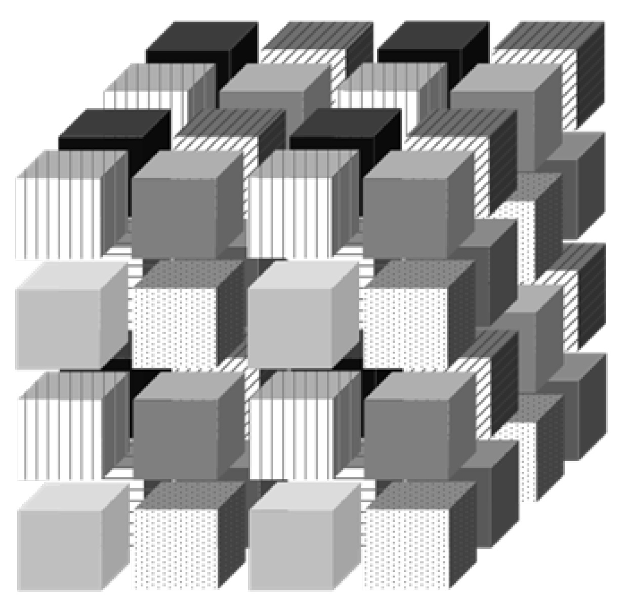
After a thorough analysis of the source code, a color block scheduling scheme is proposed. As shown in Figure 7 (with different shades of gray and fillings representing different colors), due to the three-dimensional distribution of the data structure, an original block needs to be further divided into eight smaller blocks of different colors. This ensures that adjacent small blocks have different colors. Based on this, all small blocks of the same color can be executed in parallel. Since parallel tasks are physically non-adjacent, they will never update the same data point. On the other hand, small blocks of different colors are executed serially. This guarantees the correct execution of dependencies. Listing 2 provides a detailed description of the steps involved in the execution of the color block scheduling scheme. As for load balancing, OpenMP’s dynamic scheduling is directly utilized.

Listing 2. Color block scheduling pseudo code.

The FWD operator can be directly parallelized. ADJ operator, after undergoing block pretreatment, static linked list creation, and color block scheduling, achieves successful parallelization with satisfactory results. The specific results are shown in

Table 1. Thread-level parallel effect(s).

	Random	Radial	Spiral
serial	2765	2900	2620
Multi-threaded	24.24	25.16	13.3

, where time represents the overall program execution time, measured in seconds using the rdtsc() timing function with nanosecond precision. The time units in Table 1 have been converted to seconds. The Random dataset achieved a speedup of 114×, the Radial dataset achieved a speedup of 115×, and the Spiral dataset achieved a speedup of 196×.

3.4. Vector Parallelization

3.4.1. Multiple Loop Versions

Multiple loop versions are an effective method for developing program parallelism. Some dependencies in the program are difficult to determine through static analysis alone, so the common practice is to conservatively avoid any parallelization. The multiple versions approach generates multiple code versions for different possible scenarios in the program and inserts runtime detection statements in the program to execute different program paths based on the detection results. Each path corresponds to a code version, as shown in the pseudo code in Listing 3.

Listing 3. Multi-version pseudo code.

After analysis, it was found that the two core loops in this project cannot be vectorized due to dependencies when computing on the edges of the dataset. To address this, runtime detection code is inserted to determine if the current computation is on the edge of the dataset. If it is, the original serial computation is maintained; if not, the computation can be vectorized, requiring the generation of corresponding vectorized versions.

3.4.2. Short Vector Parallelization

The outer loop is parallelized at the thread level, utilizing the multi-core computing resources. The inner loop further implements vectorization to generate vectorized parallel versions. Vectorization approach: Since multiple versions have been generated through the previous approach, which are free from dependencies, this project utilizes the SIMD compilation directive “pragma simd” in OpenMP to directly achieve program vectorization. The AVX512 instruction set with a vector width of 512 bits on the X86 platform is used for vector instructions. The vectorized program shows significant performance improvement, as shown in

Table 2. Vector level parallel effect(s).

	Random	Radial	Spiral
Multi-threaded	24.24	25.16	13.3
simd	11.5	10.9	11.05

, with time measured in seconds.

3.5. Further Optimization

Additionally, some other optimization methods were employed, although their effects are not as significant as multithreading and vectorization; they still bring about some additional acceleration. These methods mainly target the automatic optimization part of the compiler by specifying certain key parameters to assist the compiler in obtaining crucial information during intermediate code optimization, instead of relying solely on the compiler’s automatic completion.

For compiler optimization acceleration, it requires repeated attempts until the best compilation parameters are determined. This is often specific to the hardware and program being used, and these optimizations may become ineffective if the environment changes. Moreover, most compiler optimizations that can be done are already automatically enabled under the -O3 compilation option. Overall, the scope of work in this area is limited, and the effects are only incremental, rather than achieving qualitative changes. The main aspects include:

1.

Block size optimization: Due to uneven data distribution, different blocks have different load balancing and scheduling overheads. The more blocks are divided, the more balanced the load, but with increased scheduling overhead. The fewer blocks that are divided, the more imbalanced the load, but with smaller scheduling overhead. Through repeated attempts, the balance point between scheduling overhead and load balancing is found, where the overall effect is the best.

2.

Prefetch optimization: Prefetching aims to extract data that will be used from slower main memory to faster cache, reducing the latency caused by cache misses. However, excessive prefetching may pollute the cache, leading to frequent cache line replacements and slowing down the speed. Prefetching can be done at the hardware level or through compiler prefetching. The optimization in this project mainly focuses on compiler prefetching, helping the compiler better prefetch relevant data in loops. This is achieved by adding the “-qopt-prefetch[=n]” compilation option, where n represents the prefetch level (default is 2). Through experiments, it was found that the best effect is achieved when n = 3. Additionally, in the program’s source code, the “pragma prefetch a,b” compiler directive is added to instruct the compiler to prefetch specific variables a and b, preventing ineffective prefetching that may pollute the cache.

3.

Optimization of minor core code segments: The program contains some functions that account for a small percentage of the overall execution time, such as chop3D(), getScalingFunction(), etc. Optimization methods include, but are not limited to, manual vectorization, adding automatic vectorization directives, multiplication optimization, floating-point optimization, and automatic parallelization optimization. The optimization results are shown in

Table 3. Further optimize the effect (s).

	Random	Radial	Spiral
Multi-threaded + simd	11.5	10.9	11.05
Small optimize	10.1	9.94	10.41

, which demonstrates the effects after the previous optimizations, with time measured in seconds.

4. Conclusions

In this paper, the hotspots of the three-dimensional Non-Uniform Fast Fourier Transform program for MRI imaging were analyzed, bottlenecks were identified, and a series of optimizations were performed to address the issue of the convolution interpolation part being difficult to parallelize on multi-core processors. In the thread-level parallelization, block preprocessing was performed first to obtain data for each thread. Then, due to the large memory consumption, a data access method based on a static linked list was proposed and implemented, greatly reducing the memory access pressure. The second optimization approach was vector parallelization, utilizing the short vector components of the target machine and cleverly avoiding vectorization issues for edge data computations through multiple versions of code. Finally, some compiler optimizations were employed, involving repeated attempts with different compilation options to find the best ones for this program. Overall, the effects achieved are shown in

Table 4. Further optimize the effect (s).

	Random	Radial	Spiral
serial	2765	2900	2620
Multi-threaded	24.24	25.16	13.3
Multi-threaded + simd	11.5	10.9	11.05
Small optimize	10.1	9.94	10.41

.