Article

Visual Hull-Based Approach for Coronary Vessel Three-Dimensional Reconstruction

by
Dominik Bernard Lau
* and
Tomasz Dziubich
Department of Computer Architecture, Faculty of Electronics, Telecommunications and Informatics, Gdansk University of Technology, Gabriela Narutowicza 11/12, 80-233 Gdansk, Poland
*
Author to whom correspondence should be addressed.
Appl. Sci. 2025, 15(19), 10450; https://doi.org/10.3390/app151910450
Submission received: 19 August 2025 / Revised: 22 September 2025 / Accepted: 23 September 2025 / Published: 26 September 2025
(This article belongs to the Special Issue Novel Advances in Biomedical Signal and Image Processing)

Abstract

This paper addresses the problem of automatically reconstructing three-dimensional coronary vessel trees from a series of X-ray angiography images, a task which remains difficult, particularly with respect to solutions requiring no additional user input. This study analyses the performance of a visual hull-based algorithm, producing the actual positions of heart arteries in the coordinate system, which is an approach not sufficiently explored in XRA images analysis. The proposed algorithm first creates a bounding cube using a novel heuristic and then iteratively projects the cube onto preprocessed 2D images, removing points too far from the depicted arteries. The method performance is first evaluated on a synthetic dataset through a series of experiments, and for a set of common clinical angles, 3D Dice of 75.25% and 78.61% reprojection Dice is obtained, which rivals the state-of-the-art machine learning methods. The findings suggest that the method offers a promising and interpretable alternative to black box methods on the synthethic dataset in question.

1. Introduction

1.1. Justification

Cardiovascular disease is one of the most common causes of death worldwide. In 2022, the European Union recorded approximately 1.68 million deaths attributable to circulatory system diseases, representing 32.7% of the total mortality rate. The average mortality rate for IHD (codes I20 to I25 in ICD10 classification) in the EU in 2022 is estimated to be approximately 105.7 per 100,000 inhabitants [1]. The gold standard in the diagnosis of IHD are X-ray coronary angiography (XRA) and computed tomography angiography (CTA). It is estimated that approximately 1.5 million procedures are performed annually in the USA, including 600,000 XRA procedures [2]. CTA is used in preliminary diagnostics and vascular assessment, while XRA is employed in interventional cardiology (allowing for the implementation of angioplasty during the treatment—PCI). In the case of XRA, two-dimensional images are obtained from different angles, requiring the interventionalist to virtually reconstruct them into a three-dimensional image for quantitative assessment (QCA). To overcome some of the limitations of 2D QCA (e.g., foreshortening), two angiographic images (angiograms) separated by a viewing angle of ≥30° are needed for each 3D reconstruction. The 3D modeling of the coronary arterial tree can enhance the accuracy of quantitative assessments of clinical medical parameters.
Despite technological advances, XRA remains challenging due to noisy images, anatomical variability, and technological limitations [3]. Various research groups have developed reconstruction algorithms based on projective geometry. The methods come with limitations in the form of their need for precise calibration; visibility of the coronary branches; and sensitivity to foreshortening, overlapping of the vessels. Furthermore, the methods are often assessed only through the repeated reprojection of the reconstructed model onto X-ray images, due to the lack of a ground-truth 3D heart tree.

1.2. Related Works

Sarmah et al. [4] proposed a classification of three-dimensional (3D) reconstruction methods in medical imaging, emphasizing approaches that vary in methodology and application:
  • Traditional methods generally follow a sequence encompassing segmentation, registration, and surface reconstruction. Segmentation involves delineating medical images into distinct regions corresponding to specific anatomical structures, while registration aligns multiple images to establish a coherent and spatially consistent 3D representation. Surface reconstruction subsequently generates a geometric model of the organ or tissue from the acquired data. Within this framework, Active Contour Models (ACMs) and Statistical Shape Models (SSMs) are frequently employed to enhance the precision and reliability of both segmentation and reconstruction.
  • Recent advances have increasingly incorporated machine learning (ML) techniques, integrating deep neural networks at various stages of the reconstruction pipeline to improve automation and accuracy. Convolutional neural network (CNN) architectures, including U-Net, Mask R-CNN, and Mesh R-CNN, are widely applied for segmentation tasks. Generative Adversarial Networks (GANs) facilitate the generation of realistic 3D organ models, particularly when imaging data are incomplete or of suboptimal quality. Point-cloud-based reconstruction approaches further enable the direct creation of 3D surfaces from imaging-derived point clouds, providing high-fidelity geometric representations.
However, reconstruction strategies are often tailored to the unique anatomical and functional characteristics of individual human organs and the specific type of medical imaging modality employed. Currently, to overcome the aforementioned obstacles, 3D reconstruction of coronary artery trees from XRA is being achieved through the combined application of ML and projective geometry.

1.2.1. 3D Reconstruction

We can split the available methods into four categories: centerline projection methods [5,6], deformable models [7,8], hybrid ML-projection methods [9,10], and ML-only approaches [11,12,13,14].
Bappy et al. [9] presented a fully automated framework for 3D vessel reconstruction from bi-plane X-ray angiography. The method combines image de-hazing for contrast enhancement, a lightweight MultiResUNet for vessel segmentation, and shape-context–based skeleton matching with stereo triangulation for 3D centerline reconstruction. Validation on phantom and in vivo mouse data demonstrated superior segmentation accuracy (up to 98.7%) and fast computation (≈2.05 s). This method is limited by its evaluation on simple vascular models and animal data, with unproven performance in complex anatomies and lacking large-scale clinical validation. Brandby et al. [11] presented 3DAngioNet, a reconstruction algorithm based on Graph Convolutional Networks (GCNs) that utilizes bi-plane angiography. The method requires an expert to define the start and end points of the segment of interest, indicating that the reconstruction applies to individual vessel segments rather than the entire coronary vascular tree. Their method incorporate explicit projective geometry and instead treats the vessel as a graph structure, where the geometry and connectivity of the coronary tree are encoded and processed through learned message passing mechanisms. The approach begins by extracting 2D vessel centerlines from two angiographic views using a segmentation and centerline extraction pipeline. These centerlines are then converted into a correspondence graph, where nodes represent matched vessel points across views, and edges capture vessel topology. A key innovation in this work is the formulation of 3D reconstruction as a node regression problem: the GCN takes the dual-view 2D coordinates and their connectivity as input and predicts the corresponding 3D positions of each node. The model is trained end-to-end using supervised learning, using ground-truth 3D data derived from XCA examinations and annotated by medical experts.
Atli et al. [15] proposed a fully convolutional neural network to reconstruct three-dimensional coronary artery trees from synthetic X-ray angiography images. Their approach integrates segmented 2D images with corresponding pose values as inputs to a multi-input FCNN, which outputs a tubular shape representation defined by center points and radii. This method enables accurate volumetric vessel modeling and achieved a Chamfer distance of  9.98 × 10⁻³.
Finally, to address the overall lack of public data in the domain, the latest machine learning approaches such as NeCA [14] use datasets acquired through different modalities such as ImageCAS originating from computerized tomography [16].

1.2.2. Calibration

Calibration of images across projections is crucial to the problem as it may limit the maximum accuracy of the reconstruction algorithms. There are two major types of artifacts present in XRA modality—heart motion and isocenter shifts. One of the common motion compensation methods is ECG gating [17]. The approach triggers the image acquisition in a given cardiac cycle and presents the information alongside the DICOM archive. Another prospective method is presented by Schechter et al. [18]. The described 3D+t method allows for dewarping of the images to reduce the motion of the image landmarks by 84–85% (2.1–2.2 pixels). The isocenter shifts can be reduced by identifying landmarks, e.g., markers on the catheter [19]. Finally, motion artifacts can be nullified by using a specialized hardware such as G-arm [20] that allows for acquiring two X-ray images simultaneously.

1.2.3. Segmentation

The method assumes pre-segmented images, i.e., such that the image is binarized and only the pixels containing vessels remain nonzero. There have been multiple approaches for the XRA acquisition modality to achieve such data. Jun et al. [21] propose an encoder–decoder neural network, which is a variant of U-Net (T-Net), achieving 0.8319 Dice and a 0.89 f 1 score for selected segments (RCA, LAD, and LCX). Chang et al. [22] introduced SE-RegUnet: U-Net with RegNet layers [23] and reported f 1 = 0.72 for all of the visible arteries. Refs. [24,25,26] also utilized U-Net variants. Molenaar et al. [27] made use of Graph Neural Network and Vision Transformer to perform vessel segmentation. Kaur and Dong [28] introduced GradXcepUNet. Their approach prioritizes explainability of the performed segmentation while maintaining the robustness of deep learning-based methods, reaching Dice = 0.98 on the 3D-IRCADb-01 dataset.

1.3. Aim of This Work

This paper contributes novelties to three key matters in the domain of 3D reconstruction. First of all, it investigates the possibility of using visual hull-based solutions for coronary artery reconstruction, introducing a heuristic for determining the initial point cloud area and making use of the cKDTree algorithm, both ideas of which have not been applied in the domain yet. Second of all, it gives a thorough analysis of the method performance, and finally, it focuses on the verifiability and interpretability of the method results at each of its steps and gives a basis for the evaluation of future works. The approach in this article proves that the 3D reconstruction algorithms can be reliably evaluated not only through a plethora of 2D reprojection metrics but also in 3D against the ground-truth data, provided a synthetic dataset is used. The in-depth examination highlights a need for extensive calibration of the acquisition devices either before or after the angiography and presents the detrimental effects that the miscalibration has on the results’ quality.

2. Materials and Methods

2.1. Proposed Method

2.1.1. Overview

The proposed shape from the silhouette algorithm requires no further user input beyond a sequence of images, and its acquisition parameters present in the DICOM [29] files acquired as a result of the coronary artery examination, as marked on Figure 1.
The algorithm’s aim is to obtain a point cloud representing coronary vessels’ tree position during the coronary angiography. The method in question assumes the input data is segmented as shown on Figure 1, where each mask marks the pixels belonging to the vessel on the image.
The key attribute of the method is that it not only retrieves the morphological traits of the vessels’ segments but also the spatial relations between the point cloud and the characteristic points. The point cloud represents the real positions of the heart arteries during coronary angiography, enabling an enhanced visualization of the clinical procedure.
Algorithm 1 presents a pseudocode of the described method.
Algorithm 1 Method pseudocode.
1:
procedure Reconstruction(projections_and_metadata, K)
2:
     v e s s e l  CreateVoxelCube(projections_and_metadata, K)
3:
    for input_projection, metadata ∈ projections_and_metadata do
4:
         v e s s e l _ p r o j e c t i o n  Reproject( v e s s e l , m e t a d a t a )
5:
         v e s s e l  Filter( i n p u t _ p r o j e c t i o n , v e s s e l _ p r o j e c t i o n , v e s s e l )
6:
     c e n t e r l i n e s v e s s e l . c o p y ( )
7:
    for input_projection, m e t a d a t a p r o j e c t i o n s _ a n d _ m e t a d a t a  do
8:
         s k e l e t o n  Skeletonize(input_projection)
9:
         c e n t e r l i n e s _ p r o j e c t i o n  Reproject( c e n t e r l i n e s , m e t a d a t a )
10:
       c e n t e r l i n e s  FilterClosest( s k e l e t o n , centerlines_projection, c e n t e r l i n e s )
11:
    return  v e s s e l , c e n t e r l i n e s

2.1.2. First Step: Segmentation

As mentioned, the input data of the algorithm are pre-segmented images and metadata, such as primary and secondary acquisition angles, source to object distance, source to image distance, and imager spacing. While the latter is automatically acquired by the C-arm during the examination, the former is a result of processing an image. A method from Section 1.2.3 such as GradXcepUNet can be used at this point. This step will not be further discussed as it is out of the scope of this article.

2.1.3. Second Step: Initial “Cube of Interest” Construction

The next step of the algorithm is a heuristic, which to the authors’ knowledge has not been proposed in the domain. In this step, a point cloud cube of size K × K × K (with K expressed as the number of voxels) and an edge length of R meters is created and is assumed to contain the projected arteries. The following properties of the used camera model are utilized [20]:
S O D S I D = R 1 w c 2
S O D S I D = R 2 h r 2
where c , r are horizontal and vertical imager pixel spacings and w , h are width and height of the image. R 1 , R 2 are proposed edge lengths; thus,
R = m a x { R 1 , R 2 }
As the goal is to ensure the cube contains data from all of the projections, the coefficients (1) and (2) as well as the partial result (3) are computed for each input image and a maximum is chosen for the final cube construction. It must be kept in mind that the parameter K controls how precise the reconstruction will be, with K being too small causing the reconstruction to be distorted and imprecise and K too big causing the computational complexity to be too high.

2.1.4. Third Step: Point Cloud Filtering

In the next step, the created cube is sequentially projected onto input images and the points with their distances to the nearest point on the mask exceeding a given threshold are removed. To achieve that, first of all, the point cloud is rotated according to the following rotation matrix R:
R X = 1 0 0 0 c o s ( α ) s i n ( α ) 0 s i n ( α ) c o s ( α )
R Y = c o s ( β ) 0 s i n ( β ) 0 1 0 s i n ( β ) 0 c o s ( β )
R = R Y × R X
p rot = p × R T
where α , β are primary and secondary angles present in the X-ray metadata and p input point cloud R 3 . The following projection equations are then used on each rotated point:
p rot = x rot y rot z rot
c = s i d s o d + z rot
x proj = w i d t h / 2 + c x rot spacing vertical
y proj = h e i g h t / 2 + c y rot spacing horizontal
Thus, 2D projections of the point cloud on the plane that the input X-ray was acquired from are obtained (i.e., p proj = x proj y proj ). The two spacings appearing in the above equations are present in DICOM archives as “ImagerPixelSpacing” property. Finally, a CKDTree is built from the segmented vessel points belonging to the image and tests are carried out for each p proj projected earlier whether they lie within the threshold boundaries to their nearest neighbor from the CKDTree. A CKDTree serves as an index of the points, allowing for fast lookup. This part is summarized in Algorithm 2.
Algorithm 2 Filtering.
1:
procedure Filter(input_projection, vessel_projection, vessel)
2:
     t r e e  BuildCKDTree(input_projection)
3:
     q  QUERY(tree, vessel_projection, query closest points)
4:
     v e s s e l  vessel(q.distances < threshold)
5:
    return  v e s s e l
The above steps happen for each image, thus sequentially removing outlier points from the point cloud. As most of the steps are executed in parallel or using an optimized data structure, this step is efficient. The distance threshold used in the later experiments is 1 pixel, which means that only the pixels laying on the segmented arteries or in a direct neighborhood are being kept, while others are removed. This allows for a more strict evaluation of the method performance as it will be more sensitive to various noise. The described approach allows for fast filtering of not only the projected points ( p proj ) but also the corresponding points in R 3 (that is p).
To reiterate, as N images are being fed to the method, the point cloud (starting as a cube computed above) will be reprojected and filtered N times. The operation is equivalent to finding intersections of projection rays; it is however of better performance, not computing all of the possible correspondences between points [30] and being performed in parallel. As a result, after all images have been considered, the vessel point cloud is reconstructed.

2.1.5. Fourth Step (Optional): Centerline Extraction

At this point, the algorithm can be terminated and the vessel point cloud returned. Otherwise, the reconstructed vessel is forwarded to centerline extraction. In this part, the point cloud from the previous step is projected onto the images via Equation (8); however, at this point, the segmented vessel is thinned using Guo–Hall algorithm [31], which produces a skeleton or a centerline of the arteries.
Following that, another CKDTree is built, in this case, using the projected point cloud (unlike in the previous part in which the segmented vessel was used for assembling the tree). Afterwards, the CKDTree is queried for the closest neighbors to each point of the skeleton and only the closest points are kept in the point cloud. This is presented in Algorithm 3.
Algorithm 3 Filtering variant for centerline extraction.
1:
procedure FilterClosest(input_skeleton, centerlines_projection, centerlines)
2:
     t r e e  BuildCKDTree(centerlines_projection)
3:
     q  QUERY(tree, input_skeleton, query closest points)
4:
     c e n t e r l i n e s q.closest_points
5:
    return  c e n t e r l i n e s

2.2. Experiments

2.2.1. Design

A series of experiments was conducted to determine the correlation between method performance and a selected set of parameters. The following metrics, common in the domain [30,32], were taken into consideration:
  • Mean Dice coefficient ( DICE 2 D ) between reprojected point cloud and each input projection;
  • Execution time ( τ ).
Furthermore, thanks to the availability of the ground truth 3D model for the synthetic data, uncommon metrics were introduced, allowing for a more robust validation:
  • Dice coefficient in 3D ( DICE 3 D ) between the reconstructed and target point clouds;
  • IoU metric in 3D ( IoU 3 D );
  • Chamfer distance in 3D ( CD ).
The influence of the following conditions were analyzed:
  • Number of input images;
  • Patient and heart motion;
  • Vessel tortuousness;
  • Segmentation artifacts.
The quantitative assessment was performed utilizing ground truth point clouds from a synthetic dataset and the point cloud retrieved by the algorithm, having both point clouds voxelized for the comparison on each metric so that they consist of 3 × 3 × 3 [mm] vertices. The chosen voxel size does not affect morphological traits of the artery, at the same time not penalizing minor discrepancies from the ground truth, as shown by Martin et al. [33]. The size of the main coronary arteries depends on the specific vessel segment, but on average, their diameter ranges between 1 and 4 mm. Therefore, it was assumed that points are represented by a bounding neighborhood with a side length of 9 mm (corresponding to a 3 × 3 × 3 mm voxel). This allows for the detection of potential bifurcation or trifurcation points [34].

2.2.2. Datasets

For general method performance grading in perfect conditions as well as the vessel tortuousness impact study, a set of 600 vessels of different tortuousness (simple, moderate, and tortuous, 200 vessels each) was generated, for which the method was run and the metrics taken. The experiment was carried out for perpendicular projection angles as well as common clinical angles [35]. The angles used in that case were RAO 30, CRA 30; LAO 60, CRA 30; and RAO 30, CAU 30. The number of images’ influence was studied on a single vessel of moderate tortuousness: 1000 images at random angles were generated, from which 100 × N samples were taken, where N is the projection count, N { 1 15 } . The result for 100 tuples was averaged out to account for angle impact on results for each N.
Patient and heart motion were estimated by translation t r [ 100 , 100 ) 2 and scaling s [ 0.1 , 2.0 ) . The above variables were assessed separately on a single vessel. For the translation, 100 vectors from the given range were used. As for the scaling, 150 coefficient values in the above range were tested. In both cases, a single projection was translated/scaled and two more remained unaltered. The three projections were taken from perpendicular angles.
For the assessment of segmentation artifacts on the reconstruction results, a condition was introduced where each pixel can swap its value (i.e., from 1 to 0 and from 0 to 1) with a probability p. Two types of artifacts were analyzed separately: false negatives (ground truth is 1, and pixel value is 0), for which p [ 0.0 , 1.0 ) , and false positives (ground truth is 0, and pixel value is 1), for which p [ 0.0 , 0.10 ] . For both cases and each value of p, 100 different vessels were generated and three perpendicular projections taken.
For the creation of a synthetic dataset, a generator from [36] was used. The code shared by the authors was forked and restructured to a Python (3.9.13) module (The modifications are available at https://github.com/laudominik/vessel_tree_generator (accessed on 1 April 2025)). For consistency’s sake, the projection function was modified to be the same as that used in the algorithm. The tests were run on a MacBook Pro M1 (The code for the method and experiments can be found at https://github.com/cvlab-ai/visual-hull-experiments/ (accessed on 12 September 2025).

3. Results

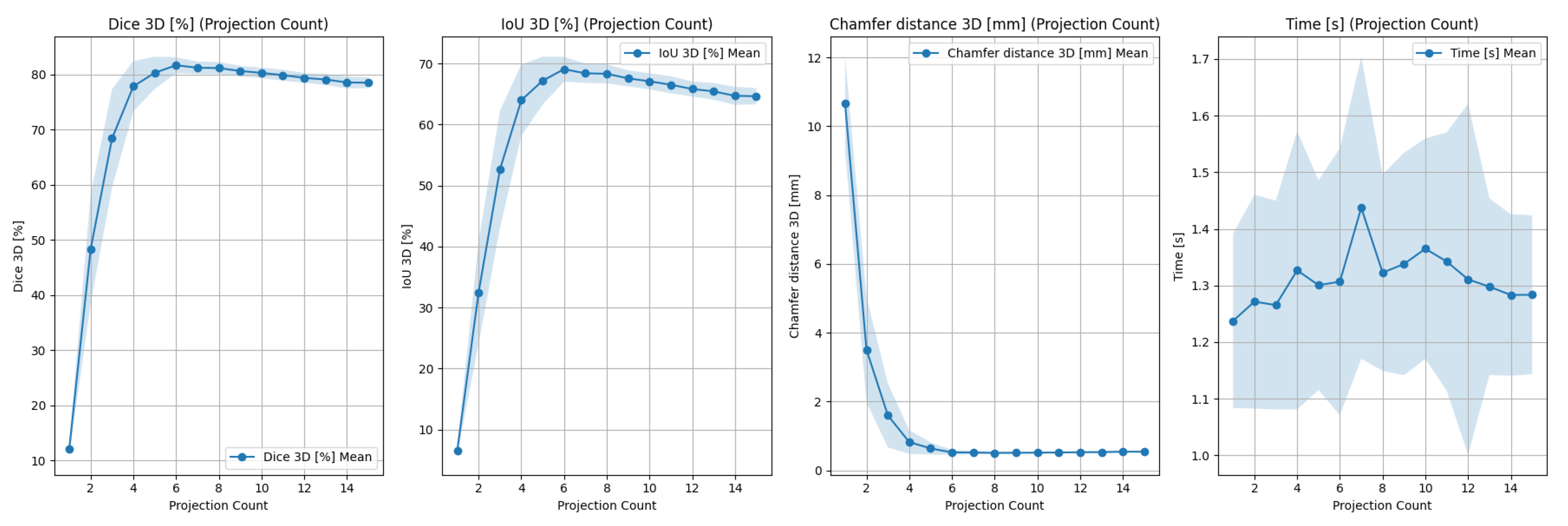
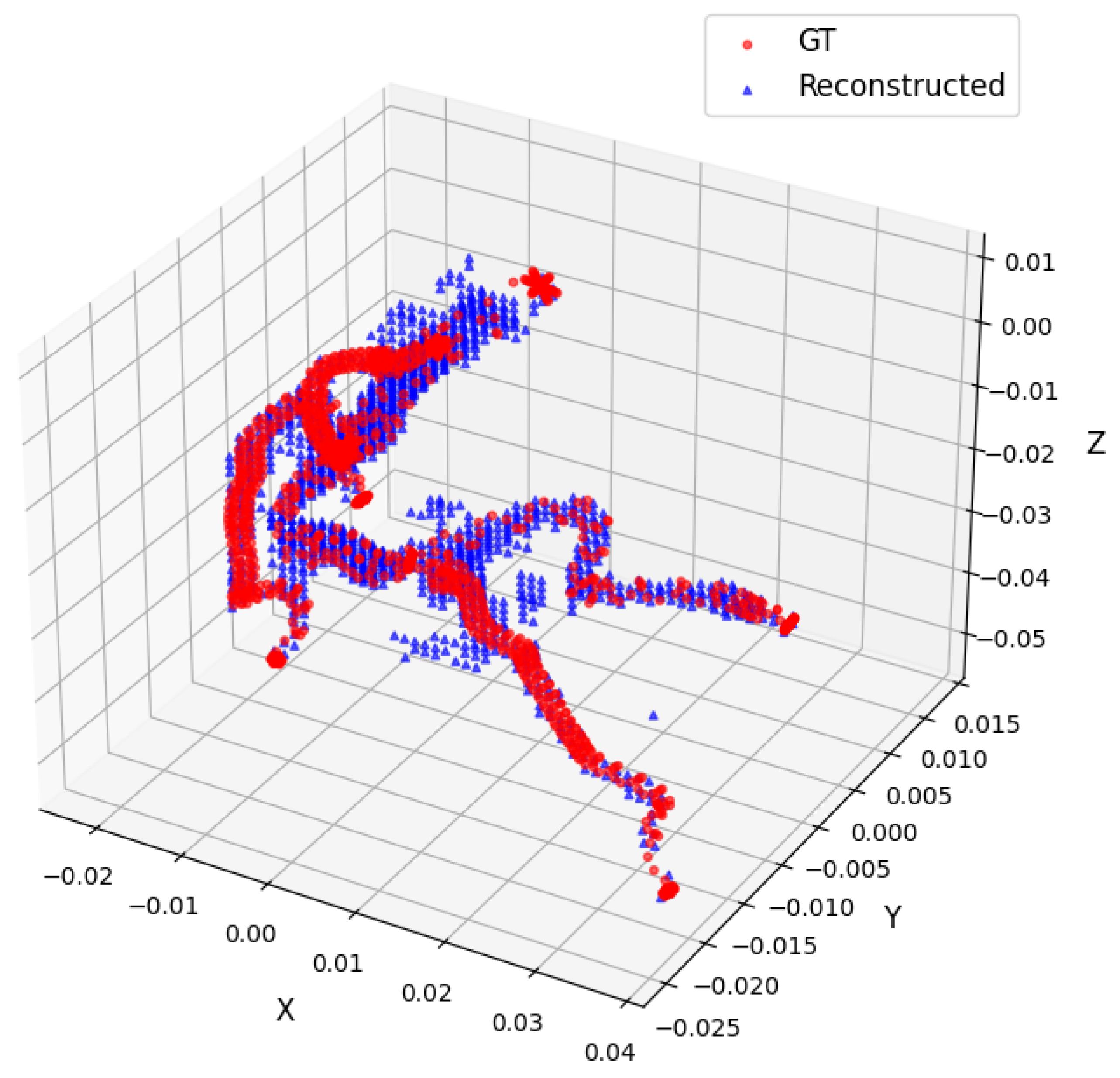
In this section, the results of the abovementioned experiments are summarized. The first experiment carried out studied the impact of input image count on reconstruction quality. The results, as well as an example reconstruction for three input projections, are shown in Figure 2.
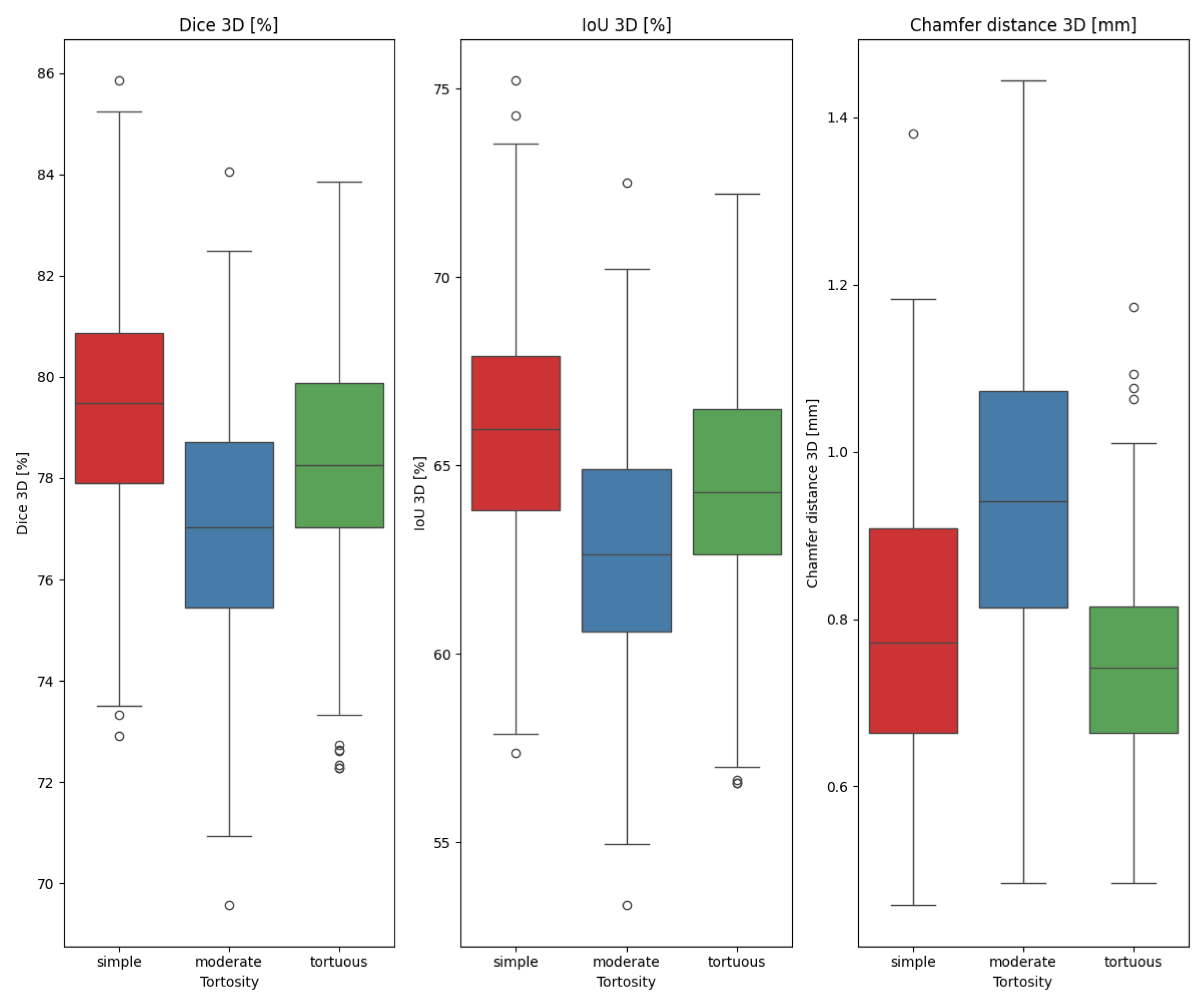
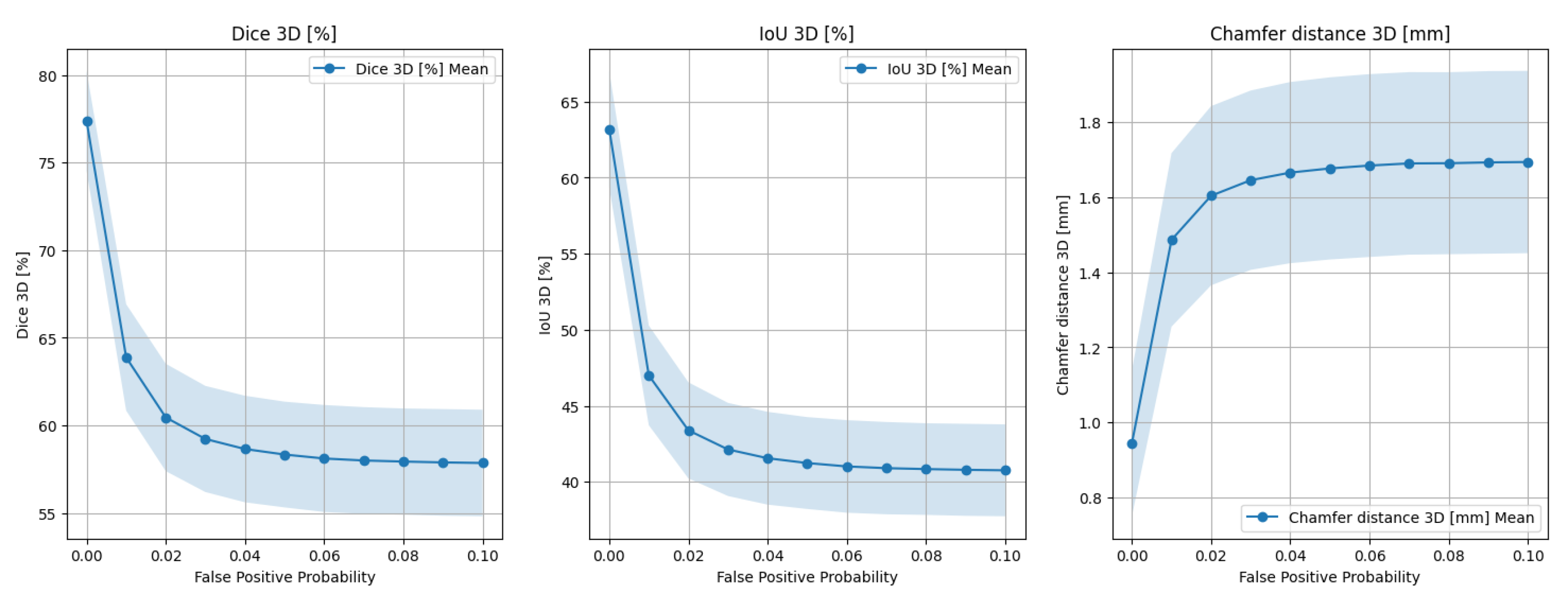
The general method performance assessment is summarized in Table 1 and Table 2, as are the box plots for each vessel tortuousness in Figure 3. The impact of translation and scaling are shown in Figure 4, and segmentation artifact influence on the metrics is presented in Figure 5 and Figure 6.

4. Discussion

In this section, a discussion, together with a statistical analysis of the results, are provided for the experimental results. The method’s general performance when perpendicular angles were used, summarized in Table 1, reaches a 2D Dice coefficient slightly lower than that for the state-of-the-art deep learning solutions [14]. As for the 3D metrics, the method reaching roughly 78% DICE and 64% IoU means the general shape of the arteries is correct. An average Chamfer distance below 1 [mm] implies that the method can be used for more precise clinical applications, given the perfect acquisition conditions. The method performance was also analyzed separately for three different vessel tortuosities. A T-test was run for each population pair, and the results are presented in Table 3. As can be implied, the differences are statistically significant, although the method performs better for vessel trees of high and low tortuousness as compared to those of moderate tortuousness. The results for common clinical angles are slightly worse than that of the perpendicular angles as the projection angles are less distinct; nevertheless, a Chamfer distance below 1 [mm] is still feasible.
As can be seen in Figure 2, the number of projections used does not significantly impact the method execution time. Mean execution time stands at μ τ = 1.313 [s], with a standard deviation of σ τ = 0.04765 . To determine the relationship between the considered variables, a regression line was fit for the relation τ ( n ) and a slope coefficient 0.002264 was obtained. A T-test was carried out with H 0 : “The residuals have a mean 0”, which resulted in a p-value of ≈1; thus, the null hypothesis was accepted. Noticeably, both the 3D Dice coefficient and IoU continue to grow, up to six projections, where maxima are reached. As for the Chamfer distance value, it also saturates at six projections. All of the metrics observe a steep improvement when increasing the projection count from one to two, although it still is not a satisfactory result. A decent reconstruction quality is reached for three projections; hence, taking into account the clinical feasibility, the optimal number of images lies in { 3 6 } . For more accurate applications it is beneficial to acquire a greater number of X-ray scans.
Given the simulation of a heartbeat (scaling) and movements between acquisitions (translations), a conclusion can be made towards the clinical usability of the method, taking into consideration the decrease in the metric values visible on Figure 4. The method suffers the most from the translation, where a cumulative 10 pixel offset drops the method performance by roughly 10% considering the Dice and IoU coefficients and about 0.5 [mm] for Chamfer distance. Above a 20 pixel offset, method performance drops below 50% Dice. The result proves the need for isocenter calibration for the method to have a use in clinical practice. The scaling does not affect the method very drastically; thus, it is of note that the performance plateaus when increasing the size of the heart, due to it being equivalent to the performance with one less image, as a larger heart mask does not introduce additional information from the projection and just contains most of the cube of interest. In both of the experiments, the metrics behave alike; however, the relationship between translation vector norm and DICE 2 D seems more linear compared to that of the 3D metrics.
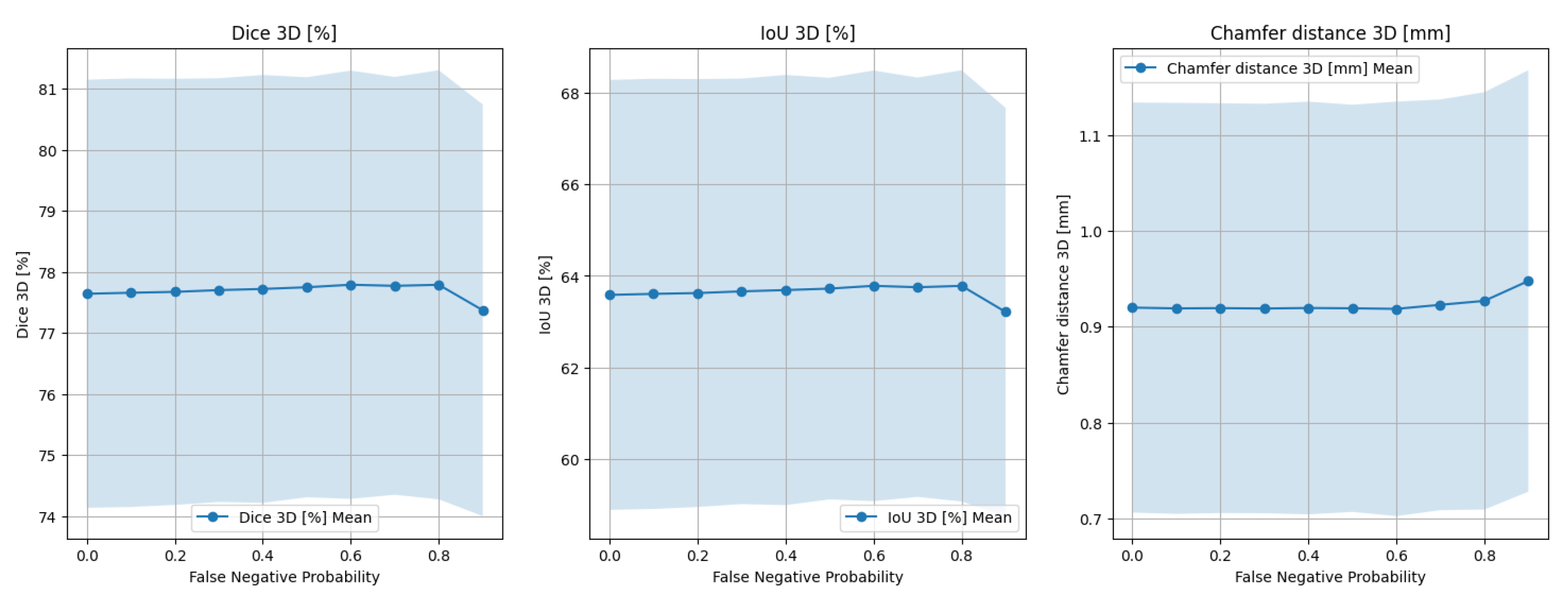
Two types of potential segmentation artifact influences were studied. False negatives were found to have little influence on the method performance, as deduced from Figure 6, which indicates the method is robust even when most of the neighboring pixels are absent. In other words, the method performance does not deteriorate greatly even when a significant fraction of pixels is removed. However, the metric values seem to deteriorate when subjected to false positives. As can be seen in Figure 5, the performance declines sharply, eventually reaching a saturation point equivalent to using one fewer projection. It must be noted, however, that the simulated artifacts appear with the same probability at each pixel, which is not always true for segmentation methods, as usually some parts of the artery tree are segmented better than the others, as demonstrated by the ARCADE challenge results [37].
Table 4 shows that the proposed method performs on par with some of the earlier ML-based approaches, while falling short of the state-of-the-art black-box methods. This depicts a trade-off between explainability and raw performance. Another highlighted trade-off is between full automation and semi-automated pipelines—semi-automatic approaches often achieve higher accuracy but require manual intervention. Fully automatic and interpretable methods are particularly well-suited for human-in-the-loop scenarios, where transparency and reproducibility are valued alongside efficiency. It should also be noted that the performance gap between methods may stem from dataset bias rather than algorithmic differences; some works report only 2D Dice scores, while others provide 3D Dice, which more directly reflects the volumetric accuracy. Finally, many machine learning methods demand heavy computational resources, which may hinder deployment in edge devices.

5. Conclusions

The presented method was thoroughly assessed on ground-truth 3D models, which is not common in research in the domain. The algorithm is fully interpretable and explainable at each step and does not require a substantial amount of data to perform at a cost of decreased performance as compared to the latest machine learning approaches, such as NeCA [14] and DeepCA [12], which both reach DICE 3 D 85 [%] being a black box method nevertheless. As for the other methods (which are not end-to-end ML), although the approaches are usually lacking a comparison to ground truth, the reprojection metrics obtained by our method are comparable to those reported by, e.g., Andrikos et al. [38], who achieved a DICE 2 D = 85 [%] for main branches. The method source code along with the test environment used for the study were entirely open-sourced for simplified reproducibility of the results. Moreover, the scalability in terms of execution time was proved, and the saturation point for a number of images being fed was determined to be around six projections. This study demonstrated that the method is robust to false negatives and maintains high sensitivity to false positives in segmentation.
It must be reiterated that the need for high calibration between the input projections might significantly limit the clinical usability of the algorithm. For that, methods such as [17,18,19] must be used. This study proves that motion and isocenter shift compensation must be used in visual hull-based methods. Finally, the work gives a quantitative benchmark for future works, not only in terms of the performance but also verifiability and explainability.
Future work of the authors will cover the integration of the developed algorithm with segmentation and calibration methods together with clinical feasibility analysis. The created pipeline will then be integrated into an existing environment for interventional cardiologists together with automatic stenosis detection and SYNTAX score computation.

Author Contributions

D.B.L.: Conceptualization, Methodology, Software, Validation, Formal Analysis, Investigation, Writing—Original Draft and Editing, Visualization; T.D.: Conceptualization, Writing—Original Draft, Review and Editing, Supervision, Validation, Data Curation. All authors have read and agreed to the published version of the manuscript.

Funding

This research was supported in part by the “Cloud Artificial Intelligence Service Engineering (CAISE) platform to create universal and smart services for various application areas” project, No. KPOD.05.10-IW.10-0005/24, as part of the European IPCEI-CIS program, financed by NRRP (National Recovery and Resilience Plan) funds.

Institutional Review Board Statement

Not applicable.

Informed Consent Statement

Informed consent was obtained from all subjects involved in this study.

Data Availability Statement

The synthetic dataset generation parameters are provided in https://github.com/cvlab-ai/visual-hull-experiments (accessed on 12 September 2025) as yaml configuration files for the provided scripts.

Conflicts of Interest

The authors declare no conflicts of interest. The funders had no role in the design of the study; in the collection, analyses, or interpretation of data; in the writing of the manuscript; or in the decision to publish the results.

Abbreviations

The following abbreviations are used in this manuscript:
SIDsource–image distance (distance between X-ray sources and the absorbing screen)
SODsource–object distance
ICDInternational Classification of Diseases
IHDIschemic Heart Disease

References

  1. ec.europa.eu. Cardiovascular Diseases Statistics. Available online: https://ec.europa.eu/eurostat/statistics-explained/index.php?title=Cardiovascular_diseases_statistics (accessed on 10 September 2025).
  2. Martin, S.S.; Aday, A.W.; Almarzooq, Z.I.; Anderson, C.A.; Arora, P.; Avery, C.L.; Baker-Smith, C.M.; Barone Gibbs, B.; Beaton, A.Z.; Boehme, A.K.; et al. 2024 Heart Disease and Stroke Statistics: A Report of US and Global Data From the American Heart Association. Circulation 2024, 149, e347–e913. [Google Scholar] [CrossRef]
  3. Cimen, S.; Gooya, A.; Grass, M.; Frangi, A.F. Reconstruction of coronary arteries from X-ray angiography: A review. Med. Image Anal. 2016, 32, 46–68. [Google Scholar] [CrossRef]
  4. Sarmah, M.; Neelima, A.; Singh, H.R. Survey of methods and principles in three-dimensional reconstruction from two-dimensional medical images. Vis. Comput. Ind. Biomed. Art 2023, 6, 15. [Google Scholar] [CrossRef] [PubMed]
  5. Vukicevic, A.M.; Çimen, S.; Jagic, N.; Jovicic, G.; Frangi, A.F.; Filipovic, N. Three-dimensional reconstruction and NURBS-based structured meshing of coronary arteries from the conventional X-ray angiography projection images. Sci. Rep. 2018, 8, 1711. [Google Scholar] [CrossRef] [PubMed]
  6. Galassi, F.; Alkhalil, M.; Lee, R.; Martindale, P.; Kharbanda, R.K.; Channon, K.M.; Grau, V.; Choudhury, R.P. 3D reconstruction of coronary arteries from 2D angiographic projections using non-uniform rational basis splines (NURBS) for accurate modelling of coronary stenoses. PLoS ONE 2018, 13, e0190650. [Google Scholar] [CrossRef] [PubMed]
  7. Lorenz, C.; von Berg, J. A comprehensive shape model of the heart. Med. Image Anal. 2006, 10, 657–670. [Google Scholar] [CrossRef]
  8. Frangi, A.; Niessen, W.; Hoogeveen, R.; van Walsum, T.; Viergever, M. Model-based quantitation of 3-D magnetic resonance angiographic images. IEEE Trans. Med. Imaging 1999, 18, 946–956. [Google Scholar] [CrossRef]
  9. Bappy, D.; Hong, A.; Choi, E.; Park, J.O.; Kim, C.S. Automated three-dimensional vessel reconstruction based on deep segmentation and bi-plane angiographic projections. Comput. Med. Imaging Graph. 2021, 92, 101956. [Google Scholar] [CrossRef]
  10. Hwang, M.; Hwang, S.B.; Yu, H.; Kim, J.; Kim, D.; Hong, W.; Ryu, A.J.; Cho, H.Y.; Zhang, J.; Koo, B.K.; et al. A Simple Method for Automatic 3D Reconstruction of Coronary Arteries From X-Ray Angiography. Front. Physiol. 2021, 12, 724216. [Google Scholar] [CrossRef]
  11. Bransby, K.M.; Tufaro, V.; Cap, M.; Slabaugh, G.; Bourantas, C.; Zhang, Q. 3D Coronary Vessel Reconstruction from Bi-Plane Angiography using Graph Convolutional Networks. arXiv 2023, arXiv:2302.14795. [Google Scholar] [CrossRef]
  12. Wang, Y.; Banerjee, A.; Choudhury, R.P.; Grau, V. DeepCA: Deep Learning-Based 3D Coronary Artery Tree Reconstruction from Two 2D Non-Simultaneous X-Ray Angiography Projections. In Proceedings of the 2025 IEEE/CVF Winter Conference on Applications of Computer Vision (WACV), Tucson, AZ, USA, 26 February–6 March 2025; IEEE: New York, NY, USA, 2025; pp. 337–346. [Google Scholar] [CrossRef]
  13. Fu, X.; Li, Y.; Tang, F.; Li, J.; Zhao, M.; Teng, G.J.; Zhou, S.K. 3DGR-CAR: Coronary artery reconstruction from ultra-sparse 2D X-ray views with a 3D Gaussians representation. arXiv 2024, arXiv:2410.00404. [Google Scholar] [CrossRef]
  14. Wang, Y.; Banerjee, A.; Grau, V. NeCA: 3D Coronary Artery Tree Reconstruction from Two 2D Projections via Neural Implicit Representation. Bioengineering 2024, 11, 1227. [Google Scholar] [CrossRef] [PubMed]
  15. Atlı, I.; Gedik, O.S. 3D reconstruction of coronary arteries using deep networks from synthetic X-ray angiogram data. Commun. Fac. Sci. Univ. Ank. Ser. A2-A3 Phys. Sci. Eng. 2022, 64, 1–20. [Google Scholar] [CrossRef]
  16. Zeng, A.; Wu, C.; Lin, G.; Xie, W.; Hong, J.; Huang, M.; Zhuang, J.; Bi, S.; Pan, D.; Ullah, N.; et al. ImageCAS: A large-scale dataset and benchmark for coronary artery segmentation based on computed tomography angiography images. Comput. Med. Imaging Graph. 2023, 109, 102287. [Google Scholar] [CrossRef]
  17. Murphy, A.; Dabirifar, S.; Feger, J. Cardiac Gating (CT). 2021. Available online: https://radiopaedia.org/articles/88788 (accessed on 14 September 2025).
  18. Shechter, G.; Shechter, B.; Resar, J.; Beyar, R. Prospective motion correction of X-ray images for coronary interventions. IEEE Trans. Med. Imaging 2005, 24, 441–450. [Google Scholar] [CrossRef]
  19. Tu, S.; Hao, P.; Koning, G.; Wei, X.; Song, X.; Chen, A.; Reiber, J.H. In vivo assessment of optimal viewing angles from X-ray coronary angiography. EuroIntervention 2011, 7, 112–120. [Google Scholar] [CrossRef]
  20. Kalmykova, M.; Poyda, A.; Ilyin, V. An approach to point-to-point reconstruction of 3D structure of coronary arteries from 2D X-ray angiography, based on epipolar constraints. Procedia Comput. Sci. 2018, 136, 380–389. [Google Scholar] [CrossRef]
  21. Jun, T.J.; Kweon, J.; Kim, Y.H.; Kim, D. T-Net: Nested encoder–decoder architecture for the main vessel segmentation in coronary angiography. Neural Netw. 2020, 128, 216–233. [Google Scholar] [CrossRef]
  22. Chang, S.S.; Lin, C.T.; Wang, W.C.; Hsu, K.C.; Wu, Y.L.; Liu, C.H.; Fann, Y.C. Optimizing ensemble U-Net architectures for robust coronary vessel segmentation in angiographic images. Sci. Rep. 2024, 14, 6640. [Google Scholar] [CrossRef]
  23. Xu, J.; Pan, Y.; Pan, X.; Hoi, S.; Yi, Z.; Xu, Z. RegNet: Self-Regulated Network for Image Classification. arXiv 2021, arXiv:2101.00590. [Google Scholar] [CrossRef]
  24. Zhu, X.; Cheng, Z.; Wang, S.; Chen, X.; Lu, G. Coronary angiography image segmentation based on PSPNet. Comput. Methods Programs Biomed. 2021, 200, 105897. [Google Scholar] [CrossRef] [PubMed]
  25. Zhao, C.; Esposito, M.; Xu, Z.; Zhou, W. HAGMN-UQ: Hyper association graph matching network with uncertainty quantification for coronary artery semantic labeling. Med. Image Anal. 2025, 99, 103374. [Google Scholar] [CrossRef] [PubMed]
  26. Zhao, C.; Xu, Z.; Jiang, J.; Esposito, M.; Pienta, D.; Hung, G.U.; Zhou, W. AGMN: Association graph-based graph matching network for coronary artery semantic labeling on invasive coronary angiograms. Pattern Recognit. 2023, 143, 109789. [Google Scholar] [CrossRef]
  27. Molenaar, M.A.; Selder, J.L.; Nicolas, J.; Claessen, B.E.; Mehran, R.; Bescós, J.O.; Schuuring, M.J.; Bouma, B.J.; Verouden, N.J.; Chamuleau, S.A.J. Current State and Future Perspectives of Artificial Intelligence for Automated Coronary Angiography Imaging Analysis in Patients with Ischemic Heart Disease. Curr. Cardiol. Rep. 2022, 24, 365–376. [Google Scholar] [CrossRef]
  28. Kaur, A.; Dong, G.; Basu, A. GradXcepUNet: Explainable AI Based Medical Image Segmentation. In Smart Multimedia; Berretti, S., Su, G.M., Eds.; Springer: Cham, Switzerland, 2022; pp. 174–188. [Google Scholar] [CrossRef]
  29. NEMA PS3/ISO 12052:2017; Digital Imaging and Communications in Medicine (DICOM). National Electrical Manufacturers Association (NEMA): Rosslyn, VA, USA, 2025.
  30. Banerjee, A.; Galassi, F.; Zacur, E.; De Maria, G.L.; Choudhury, R.P.; Grau, V. Point-Cloud Method for Automated 3D Coronary Tree Reconstruction From Multiple Non-Simultaneous Angiographic Projections. IEEE Trans. Med. Imaging 2020, 39, 1278–1290. [Google Scholar] [CrossRef]
  31. Guo, Z.; Hall, R.W. Parallel thinning with two-subiteration algorithms. Commun. ACM 1989, 32, 359–373. [Google Scholar] [CrossRef]
  32. Tsompou, P.I.; Andrikos, I.O.; Karanasiou, G.S.; Sakellarios, A.I.; Tsigkas, N.; Kigka, V.I.; Kyriakidis, S.; Michalis, L.K.; Fotiadis, D.I.; Author, S.B. Validation study of a novel method for the 3D reconstruction of coronary bifurcations. In Proceedings of the 2020 42nd Annual International Conference of the IEEE Engineering in Medicine & Biology Society (EMBC), Montreal, QC, Canada, 20–24 July 2020; pp. 1576–1579. [Google Scholar] [CrossRef]
  33. Martin, R.; Vachon, E.; Miro, J.; Duong, L. 3D reconstruction of vascular structures using graph-based voxel coloring. In Proceedings of the 2017 IEEE 14th International Symposium on Biomedical Imaging (ISBI 2017), Melbourne, VIC, Australia, 18–21 April 2017; IEEE: New York, NY, USA, 2017; pp. 1032–1035. [Google Scholar] [CrossRef]
  34. Muneeb, M.; Nuzhat, N.; Khan Niazi, A.; Khan, A.H.; Chatha, Z.; Kazmi, T.; Farhat, S. Assessment of the Dimensions of Coronary Arteries for the Manifestation of Coronary Artery Disease. Cureus 2023, 15, e46606. [Google Scholar] [CrossRef]
  35. Green, P.; Frobisher, P.; Ramcharitar, S. Optimal angiographic views for invasive coronary angiography: A guide for trainees. Br. J. Cardiol. 2016, 23, 110–113. [Google Scholar] [CrossRef]
  36. Iyer, K.; Nallamothu, B.K.; Figueroa, C.A.; Nadakuditi, R.R. A multi-stage neural network approach for coronary 3D reconstruction from uncalibrated X-ray angiography images. Sci. Rep. 2023, 13, 17603. [Google Scholar] [CrossRef]
  37. Popov, M.; Amanturdieva, A.; Zhaksylyk, N.; Alkanov, A.; Saniyazbekov, A.; Aimyshev, T.; Ismailov, E.; Bulegenov, A.; Kuzhukeyev, A.; Kulanbayeva, A.; et al. Dataset for Automatic Region-based Coronary Artery Disease Diagnostics Using X-Ray Angiography Images. Sci. Data 2024, 11, 20. [Google Scholar] [CrossRef]
  38. Andrikos, I.O.; Sakellarios, A.I.; Siogkas, P.K.; Rigas, G.; Exarchos, T.P.; Athanasiou, L.S.; Karanasos, A.; Toutouzas, K.; Tousoulis, D.; Michalis, L.K.; et al. A novel hybrid approach for reconstruction of coronary bifurcations using angiography and OCT. In Proceedings of the 2017 39th Annual International Conference of the IEEE Engineering in Medicine and Biology Society (EMBC), Jeju, Republic of Korea, 11–15 July 2017; IEEE: New York, NY, USA, 2017; pp. 588–591. [Google Scholar] [CrossRef]
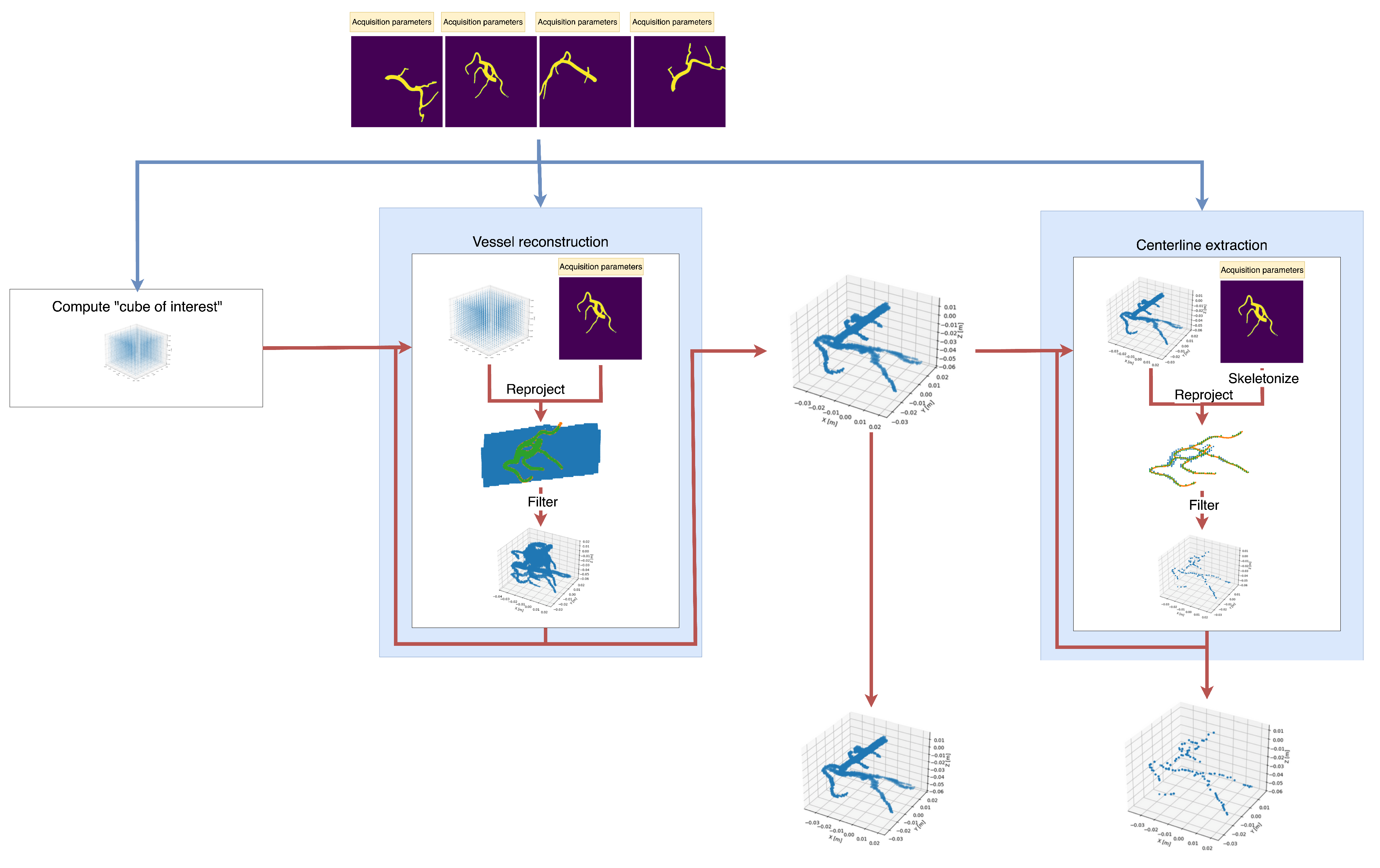
Figure 1. Proposed algorithm: Major steps and data flow of the method.
Applsci 15 10450 g001
Figure 2. Algorithm output: Performance on 3D metrics with respect to number of projections used, blue shades mark the area within one standard deviation (above). An example reconstruction for three projections (below). Input parameters: S I D = 1.2 [m], S O D = 0.8 [m], angles: { ( 0 , 0 ) , ( 0 , π 2 ) ( π 2 , 0 ) } , imager pixel spacing 0.35 [mm].
Applsci 15 10450 g002aApplsci 15 10450 g002b
Figure 3. Performance: 3D metrics for three vessel tortuosities supported by the generator.
Applsci 15 10450 g003
Figure 4. Performance: metric values with respect to scaling and translation.
Applsci 15 10450 g004
Figure 5. Performance: 3D metrics with respect to false positive occurrence probability, blue shades mark the area within one standard deviation.
Applsci 15 10450 g005
Figure 6. Performance: 3D metrics with respect to false negative occurrence probability, blue shades mark the area within one standard deviation.
Applsci 15 10450 g006
Table 1. General method performance on synthetic data with perpendicular angles and a perfect calibration in terms of mean values, standard deviation, and 95% confidence intervals.
DICE 3 D [%] IoU 3 D [%] CD [mm] DICE 2 D [%]
μ metric 78.1764.240.830778.61
σ metric 2.6603.5730.18631.095
C I μ metric 95 % (77.96, 78.38)(63.95, 64.53)(0.8157, 0.8456)(78.53, 78.70)
Table 2. General method performance on synthetic data with common clinical angles and a perfect calibration.
DICE 3 D [%] IoU 3 D [%] CD [mm] DICE 2 D [%]
μ metric 75.2560.390.999273.66
σ metric 2.6263.3750.21511.177
C I μ metric 95 % (75.04, 75.46)(60.12, 60.66)(0.9820, 1.016)(73.56, 73.75)
Table 3. p-values for each population pair with null hypotheses: H 0 : “population of tortuousness X has the same average Chamfer distance metric value as the population of tortuousness Y”.
XYp-Value
tortuoussimple0.01130
tortuousmoderate 8.507 × 10 13
simplemoderate 5.670 × 10 18
Table 4. Comparison against selected methods.
MethodResultNumber of ProjectionsArchitecture/ApproachComment
ourssee Table 1 and Table 23Sequential reprojection and filtering of the outlier points.-
[11] DICE 2 D = 87.59 [%]2Segmentation-based initialization, GCN-driven surface refinement, and branch stitching for bifurcationsIs not fully automatic (segment of interest needs to be specified). Bi-plane
[13] DICE 3 D = 70.03 [%]2U-Net to predict vessel depth from X-rays, which are then used in 3D Gaussian models.Tested on ImageCAS dataset.
[14] DICE 3 D = 90.43 [%]2Based on neural implicit representation using the multiresolution hash encoder and differentiable cone-beam forward projector layer.Tested on ImageCAS dataset.
[12] DICE 2 D 83.31 [%], CD = 3.22 [mm]2Wasserstein conditional generative adversarial network with gradient penalty, latent convolutional transformer layers, and a dynamic snake convolutional critic.Tested on ImageCAS dataset.
[33] DICE 2 D = 86.71 [%] (pulmonary), 95.85 [%] (aorta)1Random walks algorithm on a graph-based representation of a discretized visual hull.Only selected main vessels, no fine details taken into account.
[36] MSE = 0.83 [mm] (centerlines)3Feature extraction network (ResNet101) and a regular MLP (black box).Reported MSE is close to Chamfer Distance as correspondence between points is known beforehand.
[38] DICE 2 D = 85.00 [%] (main), 78.00 [%] (side)2Combining OCT-detected lumen borders with vessel centerlines derived by an expert.The second part of the algorithm is not fully automatic.
Disclaimer/Publisher’s Note: The statements, opinions and data contained in all publications are solely those of the individual author(s) and contributor(s) and not of MDPI and/or the editor(s). MDPI and/or the editor(s) disclaim responsibility for any injury to people or property resulting from any ideas, methods, instructions or products referred to in the content.