Article

A Physics-Informed Neural Network Integration Framework for Efficient Dynamic Fracture Simulation in an Explicit Algorithm

1
College of Information and Electrical Engineering, China Agricultural University, Beijing 100083, China
2
School of Ocean and Civil Engineering, Shanghai Jiao Tong University, Shanghai 200240, China
*
Author to whom correspondence should be addressed.
Appl. Sci. 2025, 15(19), 10336; https://doi.org/10.3390/app151910336
Submission received: 26 August 2025 / Revised: 17 September 2025 / Accepted: 22 September 2025 / Published: 23 September 2025
(This article belongs to the Section Mechanical Engineering)

Abstract

Featured Application

This work presents PINNI, a novel approach that is different from the traditional integral approximation methods. It employs the integrand fitting via a shallow neural network. This enables the creation of compact models, which deliver superior precision in sequential simulations, effectively addressing the limitations of neural networks in explicit algorithms and providing efficient, accurate integrand approximation for complex constitutive relations. Furthermore, PINNI is integrated into simulation code, where it replaces the mechanical integration. The application shows that this integration makes the fracture simulation results almost identical to those by conventional methods, but the computation efficiency has been significantly enhanced.

Abstract

The conventional dynamic fracture simulation by using the explicit algorithm often involves a large number of iteration computation due to the extremely small time interval. Thus, the most time-consuming process is the integration of constitutive relation. To improve the efficiency of the dynamic fracture simulation, a physics-informed neural network integration (PINNI) model is developed to calculate the integration of constitutive relation. PINNI employs a shallow multilayer perceptron with integrable activations to approximate constitutive integrand. To train PINNI, a large number of strains in a reasonable range are generated at first, and then the corresponding stresses are calculated by the mechanical constitutive relation. With the generated strains as input data and the calculated stresses as output data, the PINNI can be trained to reach a very high precision, whose relative error is about 7.8 × 10 5 %. Next, the mechanical integration of constitutive relation is replaced by the well-trained PINNI to perform the dynamic fracture simulation. It is found that the simulation results by the mechanical and PINNI approach are almost the same. This suggests that it is feasible to use PINNI to replace the rigorous mechanical integration of constitutive relation. The computational efficiency is significantly enhanced, especially for the complicated constitutive relation. It provides a new AI-combined approach to dynamic fracture simulation.

1. Introduction

The fracture simulation by the explicit integration algorithm usually involves a very large number of iteration computation due to the very short time interval, in which the most time-consuming process is the mechanical integration of constitutive relation, especially the complicated constitutive relation [1,2,3,4]. To address this problem, some scholars have developed many advanced methods to improve the computational efficiency. For instance, Noels et al. [5] developed a combined implicit–explicit algorithm to enhance the stability and efficiency in crashworthiness analysis by avoiding unnecessary iterations. In this method, they took advantage of dynamic characteristics to switch implicit and explicit algorithms where necessary. Martinez et al. [6] proposed computationally optimized formulations for explicit finite-element codes in composite delamination simulations, reducing computational demand through simplified mixing theory and layer stacking within single elements. Kuchnicki et al. [7] recast implicit constitutive integrators into explicit forms for single-crystal plasticity modeling, achieving up to 50 times faster simulations under dynamic loading while maintaining accuracy. Wang et al. [8] have conducted detailed analysis on the numerical integration efficiency. Although these methods can improve the computational efficiency to a great extent, they are intrinsically rooted in mechanics, not yet breaking through the framework of mechanics. To address this problem, new approaches that do not employ the mechanical philosophy should be explored to improve the computational efficiency.
Recently, neural network applications have advanced significantly across various disciplines in computational mechanics. The neural network model seems a promising approach to addressing this problem, e.g., [9,10,11,12,13,14]. Vu-Quoc and Humer [15] discussed hybrid approaches that combine PDE discretization with neural networks to model nonlinear constitutive relations. Herrmann and Kollmannsberger [16] categorized deep learning methods into simulation substitution, enhancement, and generative approaches, emphasizing their potential to streamline deterministic simulations. Zhang et al. [17] embedded artificial neural networks into twin cohesive zone models to predict composites fatigue delamination under various stress ratios and mode mixities. Xi et al. [18] used ANNs to inversely predict the fracture properties of concrete’s interfacial transition zone from meso-scale simulation and test data. These studies demonstrate that the neural network would play important roles in computational mechanics. Compared with the conventional neural network, the physics-informed neural network (PINN) seems a more powerful tool in computational mechanics. Hu et al. [19] used shallow PINNs to solve PDEs through incorporating surface differential operators into the loss function. Raissi et al. [20] developed hidden fluid mechanics to learn flow fields from visualizations by encoding Navier–Stokes equations into neural networks. Tran et al. [21] further leveraged PINNs constrained by the Maxwell–Betti reciprocal theorem to reconstruct the crack-tip cohesive zone law from far-field stresses and displacements, showing robustness in inverse fracture problems. Koeppe et al. [22] further proposed physics-explaining neural networks to interpret trained models for constitutive relations, bridging the black box gap in neural-network-based mechanics.
However, for the numerical simulation process that requires sequential calls but cannot be processed in large batches, the neural network struggles to leverage batch inference advantages, whereas the model complexity reduction usually leads to a decrease in accuracy [23]. To address this issue, the neural network integration method is introduced. Lloyd et al. [3] suggested that the shallow neural network can approximate smooth integrands and achieve analytical computation of the antiderivative by utilizing integrable activation function. This allows neural networks to maintain accuracy through large-batch inference over the integration domain while simultaneously reducing model complexity to enhance the inference speed during small-batch calls.
Inspired by the research mentioned above, the goal of this study is to establish a neural network model, instead of a mechanical approach, to calculate the constitutive integration in dynamic fracture simulations in order to improve the simulation efficiency. Thus, we design a general framework, termed as physics-informed neural network integration (PINNI), to create a fast and accurate model for arbitrary constitutive integrands. Once this PINNI is well trained, it is embedded into the computation code, instead of the mechanical subroutine of constitutive relation, to compute the stress with the strain input. By this method, the computational efficiency can be significantly improved. We demonstrate its effectiveness through the specific integration type of constitutive model, namely the augmented virtual internal bond model [24].

2. Methods

The mechanical constitutive relation can be written in the following form:
σ = a b g x ; ε d x
where x stands for the integration variable and ε the strain tensor.
To improve the computational efficiency of dynamic fracture simulation using an explicit algorithm, our strategy is to replace the direct mechanical constitutive integration with a highly efficient neural network model. The flowchart of this strategy is shown in Figure 1.

2.1. Physics-Informed Neural Network Integration

The main innovation of our approach lies in combining neural network integration (NNI) with physics-informed neural networks (PINNs) to form PINNI, which is used to replace the traditional numerical constitutive integration. NNI fundamentally approximates the integrand function g x ; ε with a neural network, allowing for efficient evaluation over batches of integration points. This is particularly advantageous in simulations requiring sequential, small-batch calls, as it decouples the integrand approximation from the integration step, enabling rapid inference without sacrificing accuracy. Unlike the standard neural networks, NNI leverages integrable activation functions (e.g., Tanh in our implementation) to facilitate analytical or efficient numerical antiderivative computation, as suggested by Lloyd et al. [3]. However, the pure NNI may lack physical enforcement, leading to potential inaccuracies in integral predictions.
To address this issue, we enhance NNI with PINN principles. This is done by embedding the physical information directly into the training process. The PINNI is designed to learn the functional form of the integrand g ^ x ; ε , ensuring that the approximated integrand not only fits the pointwise data but also satisfies the global physical constraints, such as the exact integral value derived from the mechanical constitutive relation. Thus, PINNI acts as a physics-aware model that accelerates computation and faithfully reflects the mechanics.
For the integrand, we employ a shallower multilayer perceptron to approximate it. The model architecture of PINNI consists of a shallow multilayer perceptron with 5 hidden layers, each containing 256 neurons to improve inference efficiency. We use the Tanh activation function to ensure smoothness and integrability. The network takes as input a concatenation of x and features derived from ε , producing a single output: the predicted integrand value g ^ x ; ε .
Formally, the neural network approximation is
g ^ x ; ε = NeuralNetwork inputs .
The integrand’s value depends on both the integration variable x and the strain tensor ε . Therefore, the neural network must receive inputs that can capture both dependencies. The sole output of network is the predicted value of the integrand g ^ at the given inputs.
To ensure physical consistency and accuracy, the model is trained using a physics-informed loss function. This approach penalizes both the local pointwise errors in fitting the integrand function and the global discrepancy in the computed integral value, thereby enforcing adherence to the underlying physical constraints. The source of physical information in this PINN framework comes from two components: (1) pointwise ground-truth values of the integrand g ^ x ; ε , sampled from the specific constitutive model, and (2) the ground-truth integral values I true , which are precomputed analytically or via high-fidelity numerical quadrature from the same constitutive model for various strain states. This dual enforcement ensures that the network learns a representation which is both locally accurate and globally consistent with the physics of the constitutive relation.
The form of the loss function is
L total = L func + λ L physic
where L func measures the pointwise fitting error, L physic enforces the integral constraint, and the hyper-parameter λ > 0 balances the relative importance of these two components.
The function fitting loss L func is computed using the Mean Squared Error between the neural network’s predictions g ^ ( x i ; ε ) and the ground-truth values g ( x i ; ε ) at a set of M training points { x i } i = 1 M :
L func = 1 M i = 1 M g ^ ( x i ; ε ) g ( x i ; ε ) 2 .
The physics-informed loss L physic penalizes the error in the integral approximation. Specifically, we sample N points { x j } j = 1 N uniformly over the integration domain [ a , b ] , evaluate the network predictions g ^ ( x j ; ε ) , and approximate the integral using the trapezoidal rule:
a b g ^ x ; ε   d x j = 1 N 1 1 2 g ^ x j + 1 ; ε + g ^ x j ; ε x j + 1 x j .
The trapezoidal rule is a classic numerical integration method that approximates the definite integral of a function over an interval by dividing the interval into N 1 equal-width subintervals (with step size Δ x = ( b a ) / ( N 1 ) ) and treating each subinterval [ x j , x j + 1 ] as a trapezoid. The area of each trapezoid, corresponding to the integral contribution of the subinterval, is calculated as Δ x / 2 g ^ ( x j ; ε ) + g ^ ( x j + 1 ; ε ) , where g ^ ( x j ; ε ) and g ^ ( x j + 1 ; ε ) are the predicted values of the integrand at the two endpoints of the subinterval. The total integral is calculated by summing the areas of all trapezoids, shown as Equation (5). In this study, the trapezoidal rule is first applied to the 1D integration scenario corresponding to Equation (1), where x is the single integration variable (1D). For this 1D case, the integration domain [ a , b ] is discretized into uniformly spaced sampling points to ensure computational simplicity and consistency with the batch inference of the neural network. Each sampling point x j is paired with strain features derived from ε as input to PINNI, and the network outputs the corresponding g ^ ( x j ; ε ) for trapezoidal summation.
This approximation is then compared to the known ground-truth integral value I true , yielding
L physic = j = 1 N 1 1 2 g ^ x j + 1 ; ε + g ^ x j ; ε x j + 1 x j I true 2 .
By minimizing L total , the neural network learns to approximate the integrand while respecting the integral constraint, improving generalization especially in data-sparse regimes.

2.2. Inference and Integration

During a simulation, to compute a stress tensor, the following steps are performed:
(1)
A dense vector of N points, x k ( k = 1 , 2 , . . . , N ) , is defined over the integration domain.
(2)
The trained neural network is queried N times, once for each point x k , while keeping the input features derived from the state ε sim constant. This yields a vector of predicted integrand values: g ^ x k ; ε sim ( k = 1 , 2 , . . . , N ) .
(3)
The integral value, I ^ ε sim is computed by applying the trapezoidal rule to this vector of integrand values.
(4)
The final stress tensor σ is then calculated from this integral.
This approach effectively decouples the integrand calculation from the integration step, replacing expensive quadrature calls with rapid batch neural network inference and a simple summation, thereby dramatically accelerating the simulation.

2.3. Validation Method

To train PINNI, a lot of data are needed. To obtain these data, we use Equation (1) to generate data to train PINNI. Firstly, we generate a sufficient number of strain tensors. These strain tensors are uniformly distributed in a reasonable range, and then the corresponding stress tensor is calculated using Equation (1). Through this method, we can obtain enough strain tensor data as input and the stress tensor as output. We use these strain and stress tensor data to train PINNI. Once PINNI is well trained, we use the well-trained PINNI to calculate the stress tensor with strain input. If the precision is high enough, we use this PINNI to replace the original mechanical constitutive relation integration in order to improve the simulation efficiency. In the following, we will use the specific constitutive relations to show how to train the PINNI and the performance of the trained-PINNI.

3. PINNI Training and Performance Check

3.1. Linear Case

In this case, we choose the basic linear elastic constitutive model, which is as follows:
σ i j = μ δ i j ε k k + 2 G ε i j ,
where μ , G are the Lame constants, and δ i j is the Kronecker delta.
To facilitate the computation by using the present PINNI, Equation (7) can be rewritten into the integral form, which is consistent with Equation (1),
σ i j = 0 1 μ   ε k k   δ i j + 2 G   ε i j   d x ,
where x [ 0 , 1 ] is a dummy integration variable (the integrand is independent of x).
To train PINNI, we first generate a sufficient number of strain tensors. In this case, a total of 5 × 10 5 strain tensors are uniformly sampled in ε i j [ 0.005 , 0.005 ] . For each strain, the integrand (constant value μ   ε k k   δ i j + 2 G   ε i j ) is sampled, and the ground-truth stress is computed via Equation (7). Here, we take Lame’s constants μ = 20 G P a and G = 15 G P a .
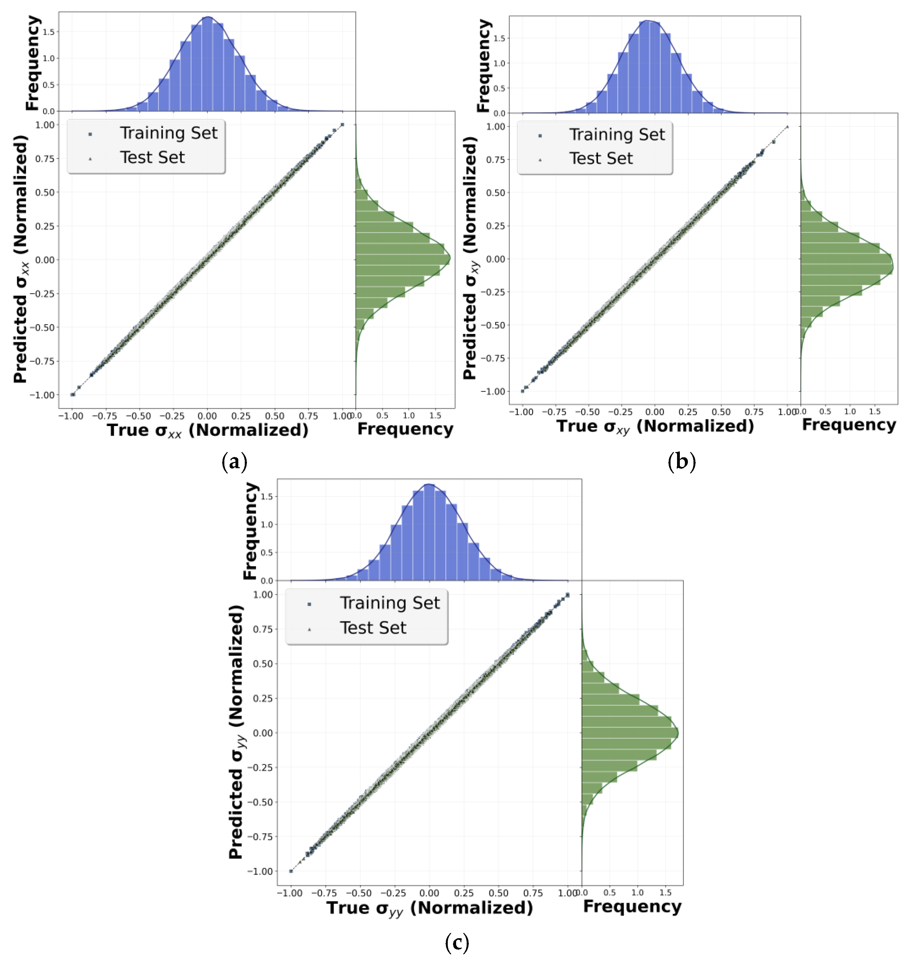
We train PINNI with the Adam optimizer (learning rate 1 × 10 3 ), 50 epochs, and loss weight λ = 0 (Equation (3)). The comparison between predicted and true integrand values for σ x x , σ x y , and σ y y components reveals near-perfect pointwise fitting, with corresponding coefficients of determination R 2 reaching 0.9992, 0.9989, and 0.9991, as shown in Figure 2. This suggests that PINNI can predict the basic linear constitutive relationship.

3.2. Nonlinear Case

3.2.1. Nonlinear Hyperelastic Constitutive Model

To further check the performance of PINNI, we choose a complicated nonlinear constitutive relation, namely the augmented virtual internal bond (AVIB) model [21]. The reason we choose AVIB as an example is two-fold. Firstly, AVIB is an integration type of constitutive relation model. Secondly, AVIB contains the micro-fracture mechanism through the bond potential. Thus, when using AVIB to simulate the fracture propagation, no external fracture criterion is needed. When and how fracture initiates, grows, and branches are completely determined by the constitutive relation. This makes the fracture propagation very simple and efficient. The series of VIB models, pioneered by Gao and Klein [25], have been extensively used to simulate fracture in different fields. The constitutive relation of AVIB has the form
σ i j = W ε i j = 1 V U Δ n Δ n ε i j + U Δ t Δ t ε i j
where W is the strain energy density, V is the volume of the micro-element, and = 0 2 π 0 π ( ) D θ , φ sin θ   d θ d φ for 3D cases and = 0 2 π ( ) D θ d θ for 2D cases in spherical coordinates. U is the bond potential; Δ n denotes the normal separation of two neighboring material particles along the direction of their bond, and Δ t is the corresponding tangential separation. They are correlated with strain tensor and bond length by
Δ n = ξ T ε ξ l 0 , Δ t 2 = ξ T ε T ε ξ ξ T ε ξ 2 l 0 2 ,
where ξ is the unit orientation vector of a bond, ξ = sin θ cos φ , sin θ sin φ , cos θ T for 3D cases, with θ , φ being the spherical coordinates and ξ = cos θ , sin θ T for 2D cases.
In AVIB, the simplified Xu–Needleman potential [26] is taken as the bond potential, which is as follows:
U ( Δ ) = ϕ n ϕ n exp Δ n δ n 1 + Δ n δ n 1 q + q exp Δ t 2 δ t 2 ,
where ϕ n stands for the work associated with normal separation Δ n ; δ n and δ t are characteristic lengths for normal and tangential separations; and q   = ϕ t / ϕ n , with ϕ t being the work associated with shear separation. The micro–macro-elastic constants are identified as
ϕ n = V δ n 2 l 0 2 3 E 4 π 1 2 ν , q = δ t 2 δ n 2 1 4 ν 2 1 + ν f or   3 D   cases , ϕ n = V δ n 2 l 0 2 E π 1 ν , q = δ t 2 δ n 2 1 3 ν 2 1 + ν f or   2 D   cases ,
For the 2D case, AVIB has the specific expression
σ i j = 1 V 0 2 π U Δ n Δ n ε i j + U Δ t Δ t ε i j d θ .
Equation (13) describes the 2D AVIB constitutive integration, where the stress σ i j is obtained by integrating the vector-valued integrand over the angular variable θ [ 0 , 2 π ] ; although this belongs to a 2D scenario, the integration itself is a 1D integral. Thus, the trapezoidal rule is extended here to compute this 1D angular integral, following the same core logic as the 1D x -integral in Equation (1) with adjustments to the integration domain and sampling strategy. Specifically, the angular interval [ 0 , 2 π ] is first uniformly divided into N sampling points θ 1 = 0 , θ 2 , , θ N = 2 π , with step size Δ θ = ( 2 π 0 ) / ( N 1 ) ; then, the trained PINNI takes the concatenation of θ j and features derived from the 2D strain tensor ε as input, and outputs the predicted vector-valued integrand,
g ^ ( θ j ; ε ) = 1 V U Δ n Δ n ε i j + U Δ t Δ t ε i j | θ j ;
Finally, for each component of the vector integrand g ^ ( θ j ; ε ) , the integral over [ 0 , 2 π ] is approximated by summing the trapezoidal areas of all subintervals [ θ j , θ j + 1 ] , which is expressed as
0 2 π g ^ ( θ ; ε ) d θ j = 1 N 1 Δ θ 2 g ^ ( θ j ; ε ) + g ^ ( θ j + 1 ; ε ) .
Substituting this approximate integral into Equation (11) yields the 2D stress σ i j , and this extension ensures that PINNI’s integration framework remains consistent across 1D and 2D modeling scenarios, leveraging the trapezoidal rule’s simplicity for 1D integrals within higher-dimensional problems.

3.2.2. Training and Accuracy Check

Indicated in Equation (13), the integrand g is a function of the integration angle θ and the strain tensor ε . Thus, the network inputs are the angle θ and the strain tensor ε . This model is trained to learn the mapping from the input space θ , ε to the integrand value g θ ; ε .
The component of strain tensor is assumed to be uniformly distributed in the range of ε i j 0.005 , 0.005 . We uniformly generate 10 6 random strain samples in the given range. For each strain sample, we perform the calculation of the integrand at a series of discrete angles θ k . This creates a training dataset of tuples: { θ k , ε , g θ k ; ε } . The model was trained using the Adam optimizer with a learning rate of 1 × 10 3 , 1000 epochs, and the loss-weighting hyperparameter λ = 0.5 .
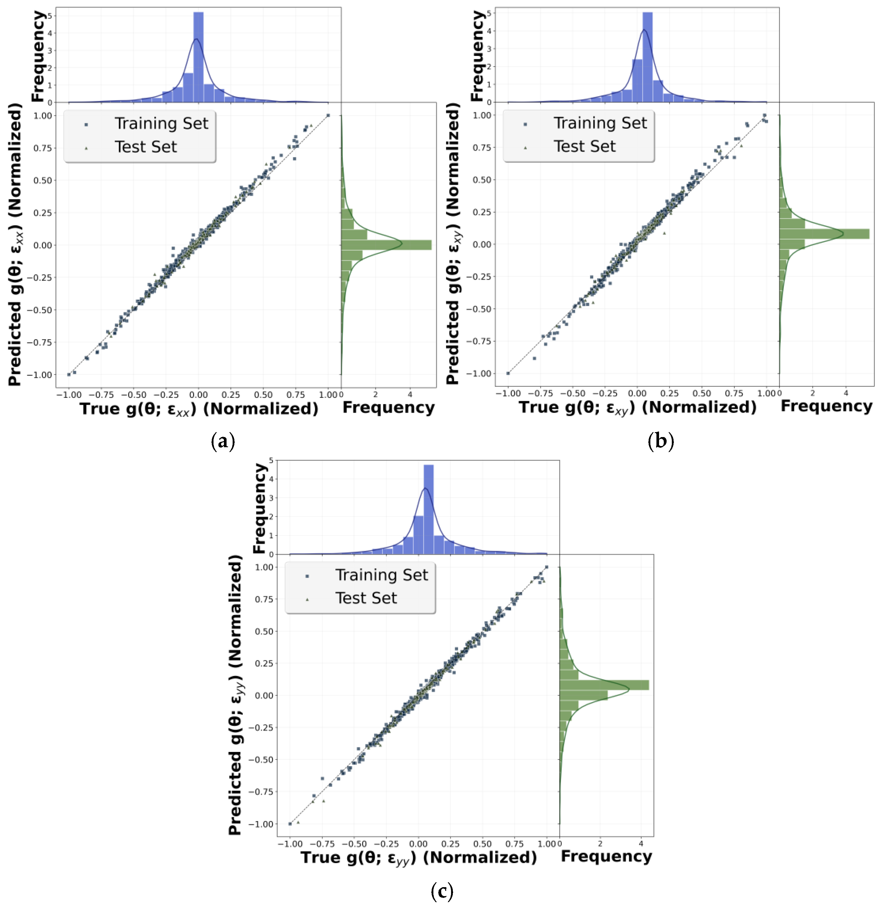
The training results are shown in Figure 3 and Table 1. From Figure 3, it can be seen that PINNI can accurately fit the integrand of the three components and demonstrates good generalization performance on the test set. Furthermore, Table 1 demonstrates the relative error of test set integration under different training samples, integrand point count N , and physics loss weight λ . The relative error gradually decreases as the training data volume and integrand points increase. Furthermore, the sensitivity analysis of λ (Table 1) shows that the average relative error follows a unimodal trend. With 1 0 6 training samples and N = 2000 , the error decreases from 4.0   × 1 0 4 at λ = 0 to a minimum of 7.8 × 1 0 5 at λ = 0.5 , then rises to 2.3 × 1 0 4 at λ = 2 . This behavior arises because λ = 0.5 optimally balances Lfunc and Lphysic. Too small a λ neglects physical constraints, while an overly large λ sacrifices local accuracy. It also indicates that the model achieves the highest accuracy when the training samples is 10 6 , N   = 2000 , and λ = 0.5 . Through the analysis above, we find that the PINNI can reach a very high precision, and the prediction of PINNI is also very stable.

3.2.3. Efficiency Check

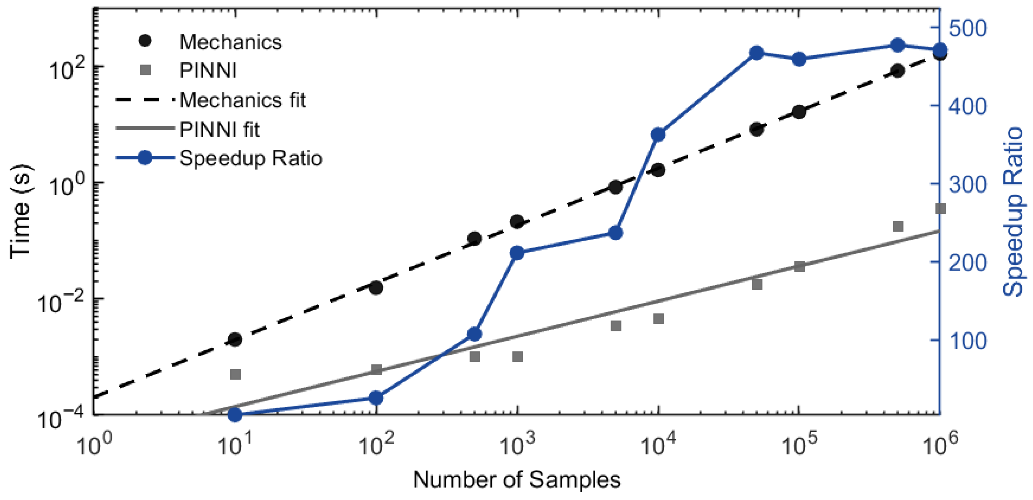
To check the efficiency of PINNI, we conducted benchmarks with AVIB constitution on specific hardware configurations: an NVIDIA RTX 4060 GPU (8 GB GDDR6 VRAM, 3072 CUDA Cores, base clock 1.83 GHz) and an Intel Core i7-13700K CPU (16 cores/24 threads, 32 GB DDR5-5600 RAM) with PyTorch 2.1. We firstly observe the computational cost of the training process: For the optimal training setup ( 10 6 strain samples, 1000 epochs, Adam optimizer with learning rate 1 × 10 3 , λ = 0.5 ), the total wall-clock time was ~1.7 h including 0.4 h for data generation and 1.3 h for GPU-based model training. Then, we calculate the stress with the same strain input for different times by the mechanics and PINNI, respectively. Shown as Figure 4, the batch benchmarks show that the neural network processes a significantly higher number of integrals per second compared to the traditional numerical integration method. Specifically, the neural network achieves a rate of approximately 1.35 million integrals s 1 , while the numerical integration processes around 9000 integrals s 1 . The speedup ratio increases with batch size, persisting at approximately 500 × for around 10 6 calls. Thus, if PINNI is introduced to the numerical simulation, the calculation speed will be improved significantly. In the explicit algorithm, it does not involve the calculation of stiffness matrix and its inverse but involves a large number of computations of constitutive relation. Therefore, the computation speed will be significantly accelerated if PINNI is used to replace the mechanical integration of constitutive relation. In such a situation, the performance of PINNI can reach its maximum.

3.3. Benchmark Comparison

To comprehensively assess the advantages of the proposed PINNI framework, we conducted benchmark comparisons against the representative surrogate model and the reduced-order model that are widely used in computational mechanics. The selection of these models covers different technical paradigms: a classical MLP regressor and a random forest regressor.
For data consistency, the same AVIB dataset described above is used for training and testing: 1 × 10 6 strain samples, with integral values sampled at 2000 discrete angular points. The dataset is divided into a training set (80%) and a test set (20%), with no overlap between the two sets.
Regarding model configuration, the neural-network-based models (PINNI and classical MLP) adopt the same shallow MLP architecture: five hidden layers, each with 256 neurons, and a Tanh activation function. The random forest regressor, as a non-neural-network baseline, is configured with 100 decision trees and a maximum depth of 20. In terms of training parameters, all neural network models use the Adam optimizer with an initial learning rate of 1 × 10 3 .
We used the same computational platform mentioned above, and all models were implemented in PyTorch or scikit-learn. Table 2 summarizes the accuracy and physics-informed consistency metrics of all models on the test set. PINNI achieved the highest prediction accuracy. In contrast, the classical MLP and the random forest regressor exhibit a significant performance gap.

4. Simulation Example

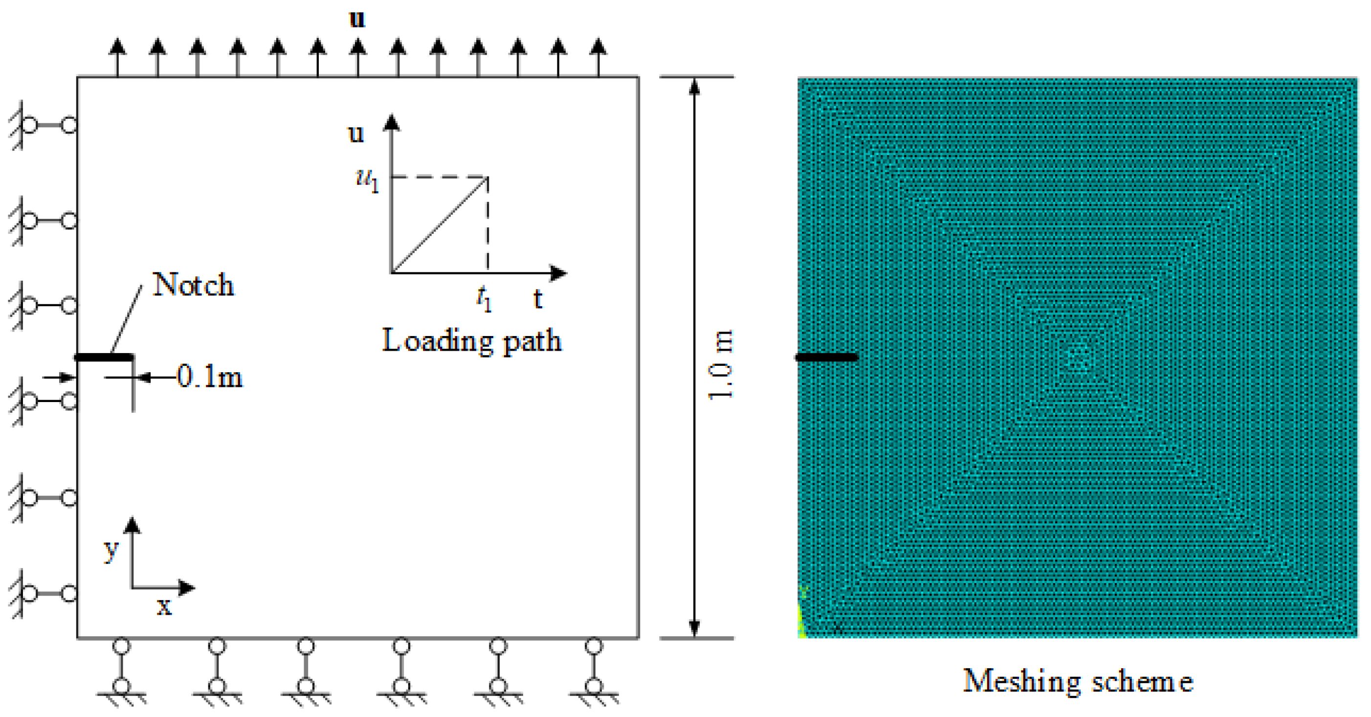
Since PINNI can predict the constitutive relation, we embed the trained PINNI into the computation code to simulate the mechanical process. To examine whether this approach is feasible, we simulate a dynamic fracture propagation example. Here, we use the AVIB constitutive model. The simulation object is a square plate with dimensions of 1   m   ×   1   m , shown in Figure 5. On the left side, there is a notch, with a length of 0.1 m. The unstructured triangular mesh is adopted. The total node number is 46,221, and the total element number is 91,640. The left and the bottom boundary are normally restricted. The displacement-controlled loading scheme is applied on the top boundary, whose loading speed is a constant, u t = 0.1   m s . In this simulation, we apply the total displacement u 1 = 0.25   mm at the time t 1 = 2.5 ms . The material parameters are as follows: Young’s modulus E = 40 GPa, Poisson ratio ν = 0.25, critical normal strain δ ~ n = 0.5 × 1 0 3 , critical shear strain δ ~ t = 0.5 × 1 0 3 , and material density ρ = 2400 kg m 3 . The explicit algorithm is employed with the time interval Δ t = 0.5 × 1 0 6   s .
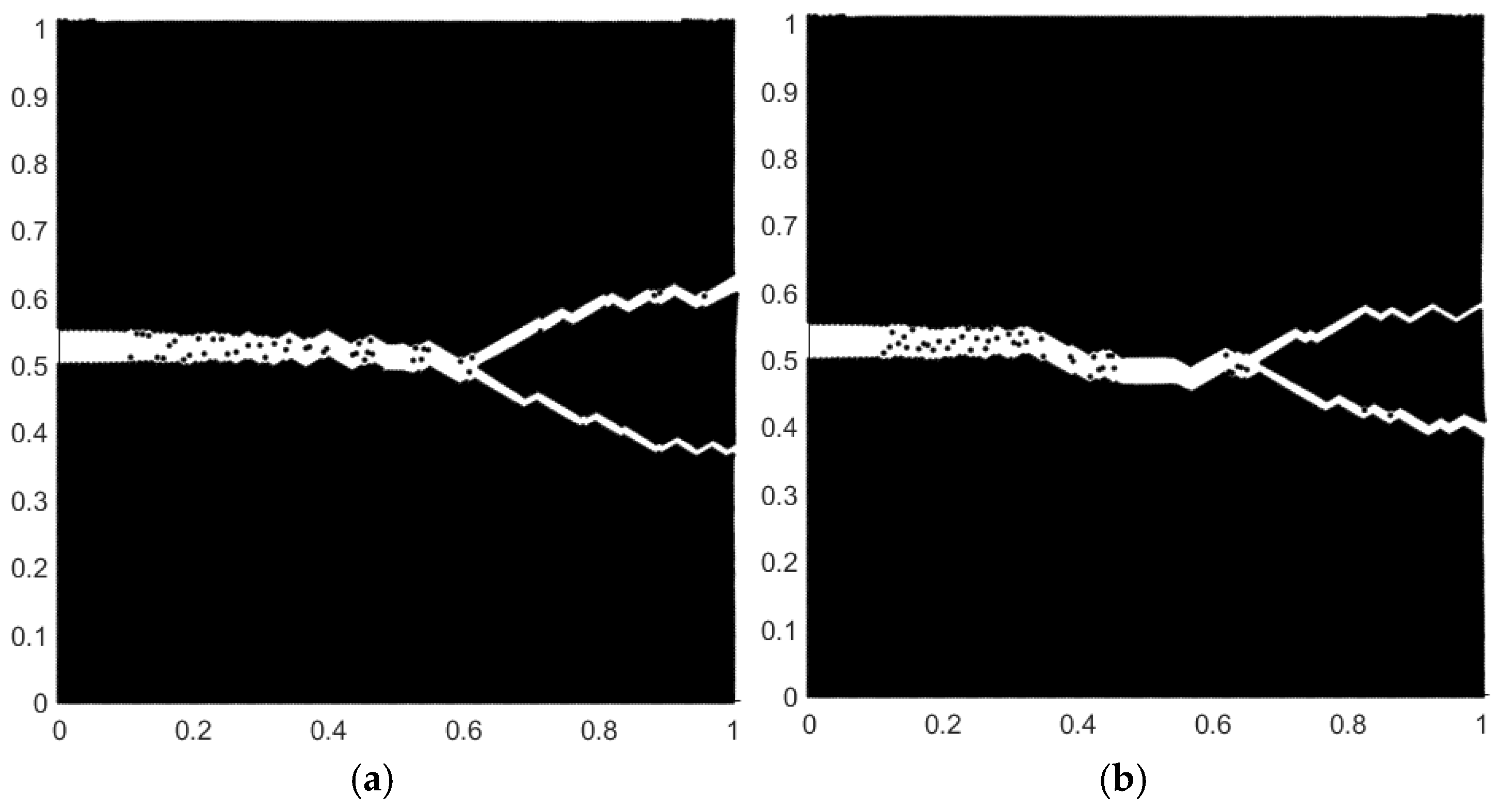
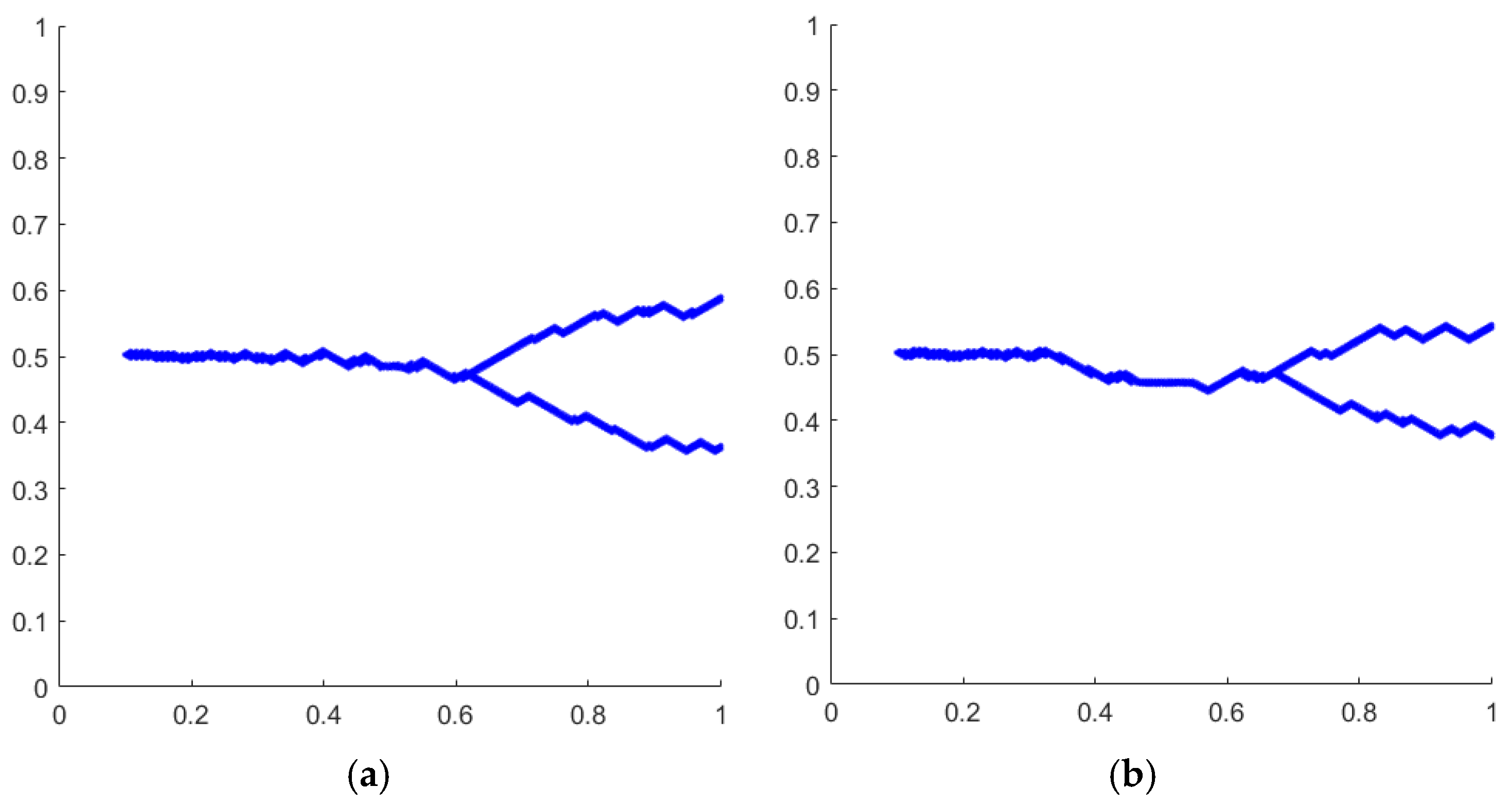
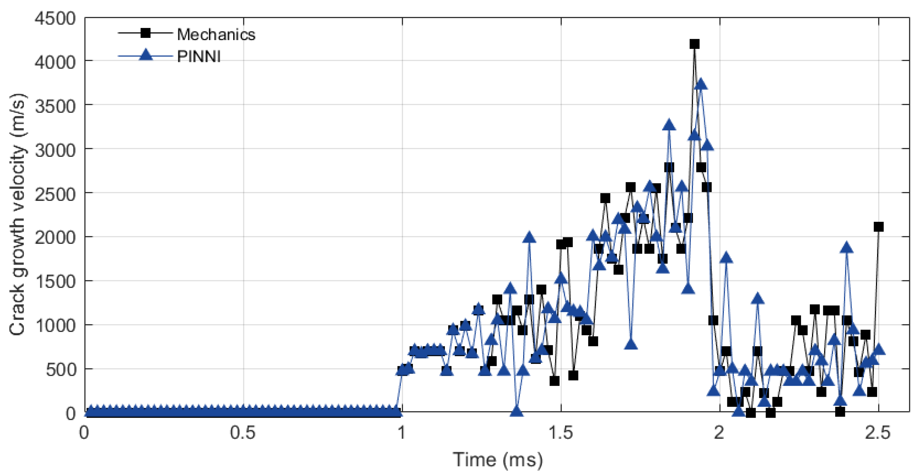
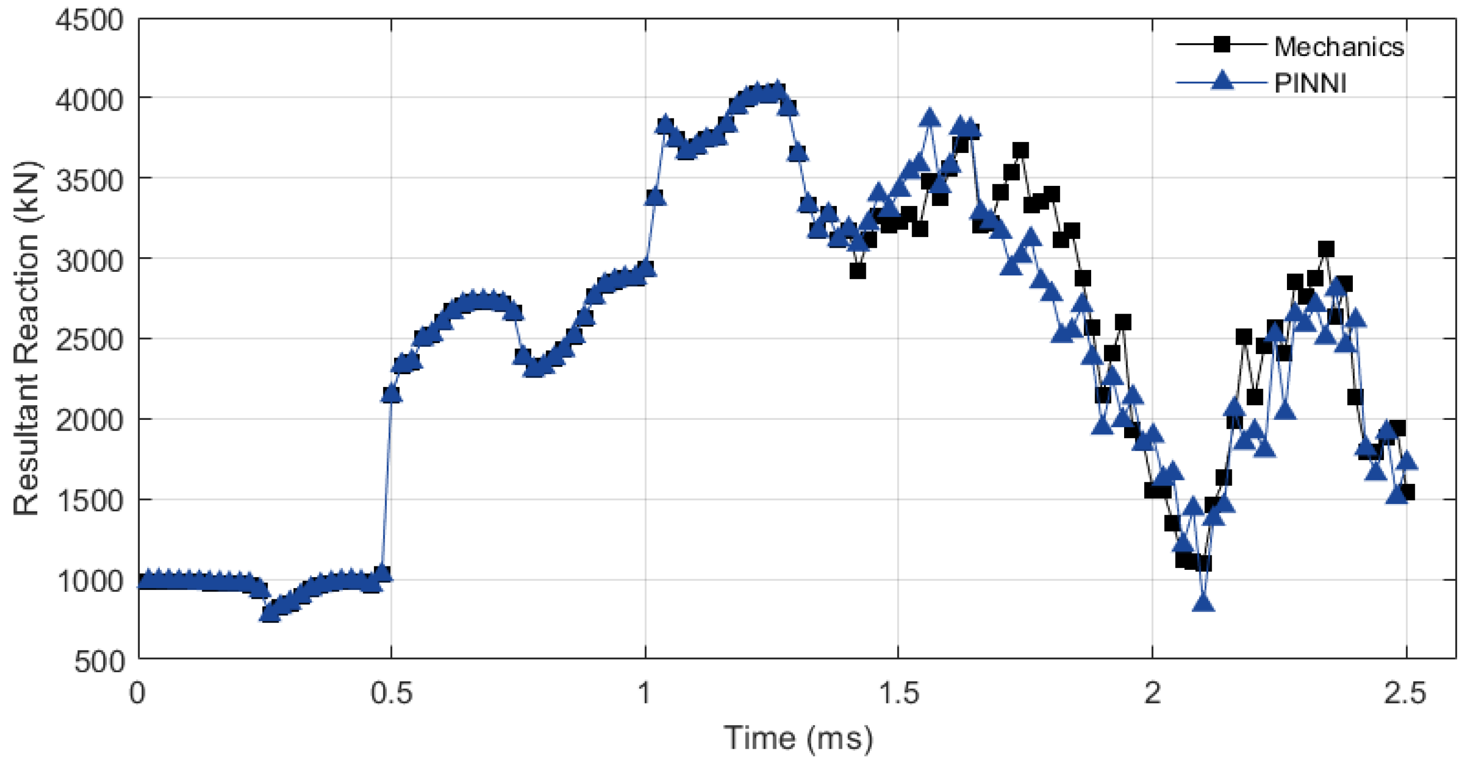
To facilitate the comparison between the mechanical and PINNI approach, we simulate this case through the mechanical AVIB and PINNI approach, respectively. The simulation results are shown in Figure 6, Figure 7, Figure 8 and Figure 9.
The simulated deformed mesh is shown in Figure 6. From Figure 6, it can be seen that the fracture propagates in a mirror manner at the beginning, then propagates in a zigzag manner, and finally branches. These are the typical features of dynamic fracture propagation. Comparing the simulated result by the mechanics and PINNI, we can find that the deformed mesh configurations are very similar, almost the same. If we extract the failed elements and plot them in a figure, the fracture trajectory can be clearly presented, shown in Figure 7. From Figure 7, it is found that the trajectories simulated by the two methods are almost the same.
To quantitatively compare the results by the two methods, we present the fracture growth velocity in Figure 8. From Figure 8, it can be seen that the growth velocities almost overlap. If we take the result by the mechanical approach as the standard one, the relative error of the result by PINNI is 0.001254. It is noted that the crack growth velocity abruptly increases between 1.5 ms and 2 ms. This is because the fracture branches. The velocity is the summation of two branches of fractures.
To further make quantitative comparison, we plot the resultant reactions on the top boundary in Figure 9. It shows that the reaction on the top also almost overlaps. The relative error of the simulated result by PINNI is 5.2 × 1 0 5 . This suggests that the PINNI can reach the same precision as the mechanical approach. Thus, the PINNI approach is feasible and reliable in dynamic fracture simulation.

5. Discussion

The key requirements for applying PINNI in industrial settings lie in balancing training costs, hardware accessibility, and scalability to large-scale dynamic fracture problems. Regarding training costs, although 1 0 6 samples are needed to achieve the best accuracy, this is only a one-time investment, requiring just 1.7 h on a mid-range GPU. For scenarios with lower accuracy requirements, reducing the number of samples to 1 0 5 can shorten the training time to 0.13 h while maintaining an error of < 6 × 1 0 3 %, which aligns with industrial cost expectations. For large-scale problems, PINNI expands through two avenues: (1) Data generation: As all PINNI data can be generated by traditional numerical methods, it is easy to extend the dataset to industrially relevant strain ranges. Thus, the model’s accuracy is effectively guaranteed over a wide range. (2) Efficient inference: By encapsulating PINNI’s inference module into a C++ dynamic link library compatible with industrial FEM tools, the speed and compatibility can be further improved.
Benchmark comparisons with other surrogate models further confirm the PINNI’s competitiveness. Relative to the classical MLP and random forest, PINNI achieves a 19× and 790× reduction in average relative error, respectively. This results from the integration of physics constraints that avoid non-mechanical predictions. For the practical dynamic fracture simulation, PINNI’s balance of speed, accuracy, and consistency makes it more suitable than the existing surrogate approaches.
The present model also has certain limitations. Firstly, it is only applicable to the linear or hyperelastic constitutive model. This is because the present PINNI cannot remember the stress (or deformation) history. It cannot account for the effect of loading history. In the elastoplastic constitutive model, the stress history must be accounted for. Thus, the present PINNI is not applicable to the elastoplastic model or path-dependent models.

6. Conclusions

In this study, a general physics-informed neural network integration (PINNI) method is proposed to accelerate the evaluation of complex constitutive integrals in computational mechanics. This framework combines neural network integration (NNI) with physics-informed neural networks (PINNs) by approximating the integrand through a shallow multilayer perceptron with integrable activation functions. It is trained with a loss function that enforces both pointwise data fitting and global integral constraints for enhanced physical consistency and accuracy.
The well-trained PINNI has very high efficiency and precision in computation of constitutive relation. Then, the PINNI is embedded into the computation code to replace the mechanical constitutive relation to simulate the dynamic fracture propagation. It is found that the simulation results by the PINNI are almost the same as that by the mechanical approach. The computational efficiency by PINNI is significantly improved in the fracture simulation with the explicit algorithm. Thus it provides a new AI-combined method for fracture simulation.

Author Contributions

Conceptualization, Z.Z. and M.W.; methodology, M.W. and Z.Z.; software, M.W. and Z.Z.; validation, Z.Z. and M.W.; formal analysis, M.W.; resources, Z.Z.; data curation, Z.Z. and M.W.; writing—original draft preparation, M.W.; writing—review and editing, Z.Z. and Y.P.; visualization, M.W. and Z.Z.; supervision, Z.Z. and Y.P.; project administration, Z.Z. and Y.P. All authors have read and agreed to the published version of the manuscript.

Funding

This research received no external funding.

Data Availability Statement

The code of this work can be found at https://github.com/mingyang-Wan/PINNI (accessed on 15 September 2025).

Conflicts of Interest

The authors declare no conflicts of interest.

Abbreviations

The following abbreviations are used in this manuscript:
PINNPhysics-informed neural network
NNINeural network integration
AVIBAugmented virtual internal bond

References

  1. Sánchez, P.J.; Huespe, A.E.; Oliver, J. On some topics for the numerical simulation of ductile fracture. Int. J. Plast. 2008, 24, 1008–1038. [Google Scholar] [CrossRef]
  2. Besson, J. Continuum models of ductile fracture: A review. Int. J. Damage Mech. 2010, 19, 3–52. [Google Scholar] [CrossRef]
  3. Lloyd, S.; Irani, R.A.; Ahmadi, M. Using neural networks for fast numerical integration and optimization. IEEE Access 2020, 8, 84519–84531. [Google Scholar] [CrossRef]
  4. Hassan, A.; Aljawad, M.S.; Mahmoud, M. An artificial intelligence-based model for performance prediction of acid fracturing in naturally fractured reservoirs. ACS Omega 2021, 6, 13654–13670. [Google Scholar] [CrossRef] [PubMed]
  5. Noels, L.; Stainier, L.; Ponthot, J.P. Combined implicit/explicit algorithms for crashworthiness analysis. Int. J. Impact Eng. 2004, 30, 1161–1177. [Google Scholar] [CrossRef]
  6. Martinez, X.; Rastellini, F.; Oller, S.; Flores, F.; Oñate, E. Computationally optimized formulation for the simulation of composite materials and delamination failures. Compos. Part B Eng. 2011, 42, 134–144. [Google Scholar] [CrossRef]
  7. Kuchnicki, S.N.; Cuitiño, A.M.; Radovitzky, R.A. Efficient and robust constitutive integrators for single-crystal plasticity modeling. Int. J. Plast. 2006, 22, 1988–2011. [Google Scholar] [CrossRef]
  8. Wang, J.; Lu, L.; Zhu, F. Efficiency analysis of numerical integrations for finite element substructure in real-time hybrid simulation. Earthq. Eng. Eng. Vib. 2018, 17, 73–86. [Google Scholar] [CrossRef]
  9. Perera, R.; Agrawal, V. Multiscale graph neural networks with adaptive mesh refinement for accelerating mesh-based simulations. Comput. Methods Appl. Mech. Engrg. 2024, 429, 117152. [Google Scholar] [CrossRef]
  10. Aldakheel, F.; Satari, R.; Wriggers, P. Feed-forward neural networks for failure mechanics problems. Appl. Sci. 2021, 11, 6483. [Google Scholar] [CrossRef]
  11. Baek, J.; Chen, J.-S. A neural network-based enrichment of reproducing kernel approximation for modeling brittle fracture. Comput. Methods Appl. Mech. Eng. 2024, 419, 116590. [Google Scholar] [CrossRef]
  12. Goswami, S.; Anitescu, C.; Chakraborty, S.; Rabczuk, T. Transfer learning enhanced physics informed neural network for phase-field modeling of fracture. Theor. Appl. Fract. Mech. 2020, 106, 102447. [Google Scholar] [CrossRef]
  13. van de Weg, B.P.; Greve, L.; Andres, M.; Eller, T.; Rosic, B. Neural network-based surrogate model for a bifurcating structural fracture response. Eng. Fract. Mech. 2021, 241, 107424. [Google Scholar] [CrossRef]
  14. Horvat, C.; Roach, L.A. WIFF1.0: A hybrid machine-learning-based parameterization of wave-induced sea ice floe fracture. Geosci. Model Dev. 2022, 15, 803–814. [Google Scholar] [CrossRef]
  15. Vu-Quoc, L.; Humer, A. Deep learning applied to computational mechanics: A comprehensive review, state of the art, and the classics. CMES Comput. Model. Eng. Sci. 2023, 137, 1070–1343. [Google Scholar] [CrossRef]
  16. Herrmann, L.; Kollmannsberger, S. Deep learning in computational mechanics: A review. Comput. Mech. 2024, 74, 281–331. [Google Scholar] [CrossRef]
  17. Zhang, B.; Allegri, G.; Hallett, S.R. Embedding artificial neural networks into twin cohesive zone models for composites fatigue delamination prediction under various stress ratios and mode mixities. Int. J. Solids Struct. 2022, 236-237, 111311. [Google Scholar] [CrossRef]
  18. Xi, X.; Yin, Z.Q.; Yang, S.T.; Li, C.Q. Using artificial neural network to predict the fracture properties of the interfacial transition zone of concrete at the meso-scale. Eng. Fract. Mech. 2021, 242, 107488. [Google Scholar] [CrossRef]
  19. Hu, W.F.; Shih, Y.J.; Lin, T.S.; Lai, M.C. A shallow physics-informed neural network for solving partial differential equations on static and evolving surfaces. Comput. Methods Appl. Mech. Eng. 2024, 418, 116486. [Google Scholar] [CrossRef]
  20. Raissi, M.; Yazdani, A.; Karniadakis, G.E. Hidden fluid mechanics: Learning velocity and pressure fields from flow visualizations. Science 2020, 367, 1026–1030. [Google Scholar] [CrossRef] [PubMed]
  21. Tran, H.; Gao, Y.F.; Chew, H.B. Numerical and experimental crack-tip cohesive zone laws with physics-informed neural networks. J. Mech. Phys. Solids 2024, 193, 105866. [Google Scholar] [CrossRef]
  22. Koeppe, A.; Bamer, F.; Selzer, M.; Nestler, B.; Markert, B. Explainable artificial intelligence for mechanics: Physics-explaining neural networks for constitutive models. Front. Mater. 2022, 8, 834946. [Google Scholar] [CrossRef]
  23. Krizhevsky, A. One weird trick for parallelizing convolutional neural networks. arXiv 2014, arXiv:1404.5997. [Google Scholar] [CrossRef]
  24. Zhang, Z.N.; Gao, H.J. Simulating fracture propagation in rock and concrete by an augmented virtual internal bond method. Int. J. Numer. Anal. Methods Geomech. 2012, 36, 459–482. [Google Scholar] [CrossRef]
  25. Gao, H.J.; Klein, P. Numerical simulation of crack growth in an isotropic solid with randomized internal cohesive bond. J. Mech. Phys. Solids 1998, 46, 187–218. [Google Scholar] [CrossRef]
  26. Xu, X.P.; Needleman, A. Numerical simulations of fast crack growth in brittle solids. J. Mech. Phys. Solids 1994, 42, 1397–1434. [Google Scholar] [CrossRef]
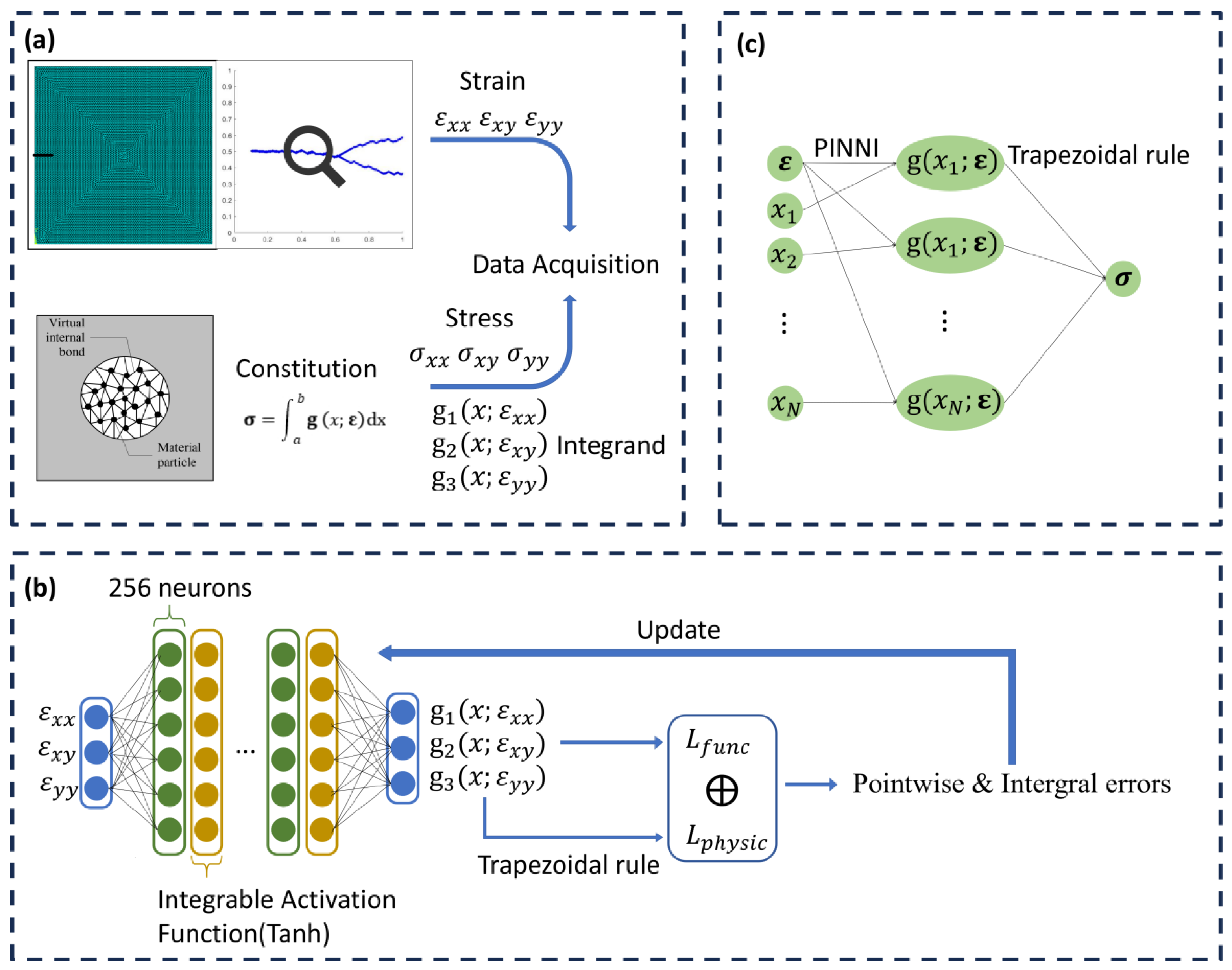
Figure 1. Flowchart of PINNI strategy. (a) Data acquisition. (b) Framework of PINNI. (c) Inference and integration computational graph.
Applsci 15 10336 g001
Figure 2. Comparison between the predicted values and the true ones. The components and training set coefficients of determination ( R 2 ) corresponding to the three subgraphs are (a) σ x x , R 2 = 0.9992; (b) σ x y , R 2 = 0.9989; (c) σ y y , R 2 = 0.9991.
Applsci 15 10336 g002
Figure 3. Comparison between the predicted integrand values and the true ones. The components and training set coefficients of determination ( R 2 ) corresponding to the three subgraphs are (a) g ( θ , ε x x ) , R 2 = 0.9940; (b) g ( θ , ε x y ) , R 2 = 0.9888; (c) g ( θ , ε y y ) , R 2 = 0.9940, with physics loss weight λ = 0.5 .
Applsci 15 10336 g003
Figure 4. Performance comparison of numerical integration and neural network inference.
Applsci 15 10336 g004
Figure 5. Simulation object and meshing scheme for dynamic fracture propagation.
Applsci 15 10336 g005
Figure 6. Simulated deformed mesh configuration (a) by mechanics and (b) by PINNI. The nodal displacement is magnified 400 times.
Applsci 15 10336 g006
Figure 7. Simulated fracture trajectory (a) by mechanics and (b) by PINNI.
Applsci 15 10336 g007
Figure 8. Comparison between the fracture growth velocity simulated by mechanics and PINNI.
Applsci 15 10336 g008
Figure 9. Comparison between the resultant reactions of the top boundary simulated by mechanics and PINNI.
Applsci 15 10336 g009
Table 1. Impact of training samples, integrand point count ( N ), and physics loss weight λ on average relative error (%).
Training Samples N λ
00.10.512
1 × 10 4 502.01.71.31.62.0
1001.19.0 × 10−16.5 × 10−18.2 × 10−11.1
2003.2 × 10−12.6 × 10−12.9 × 10−13.1 × 10−13.4 × 10−1
5001.1 × 10−19.0 × 10−28.5 × 10−29.5 × 10−21.2 × 10−1
10004.0 × 10−23.2 × 10−22.8 × 10−23.0 × 10−24.5 × 10−2
20001.5 × 10−21.2 × 10−21.0 × 10−21.1 × 10−21.8 × 10−2
1 × 10 5 509.8 × 10−18.2 × 10−14.7 × 10−15.7 × 10−17.8 × 10⁻¹
1005.2 × 10−14.2 × 10−11.9 × 10−12.3 × 10−13.2 × 10−1
2001.8 × 10−11.4 × 10−15.0 × 10−29.0 × 10−21.2 × 10−1
5005.5 × 10−24.2 × 10−22.0 × 10−22.8 × 10−24.0 × 10−2
10001.8 × 10−21.4 × 10−27.0 × 10−31.0 × 10−21.5 × 10−2
20006.0 × 10−34.6 × 10−32.5 × 10−33.2 × 10−35.0 × 10−3
5 × 10 5 506.2 × 10−14.8 × 10−12.3 × 10−12.5 × 10−13.9 × 10⁻¹
1003.0 × 10−12.2 × 10−18.5 × 10−29.0 × 10−21.4 × 10−1
2001.0 × 10−17.4 × 10−23.2 × 10−23.7 × 10−25.3 × 10−2
5003.0 × 10−22.2 × 10−21.2 × 10−21.4 × 10−22.0 × 10−2
10001.0 × 10−27.5 × 10−34.0 × 10−34.8 × 10−37.0 × 10−3
20003.4 × 10−32.6 × 10−31.5 × 10−31.8 × 10−32.9 × 10−3
1 × 10 6 503.1 × 10−12.5 × 10−12.1 × 10−12.3 × 10−12.8 × 10⁻¹
1001.5 × 10−11.3 × 10−11.2 × 10−11.2 × 10−11.4 × 10−1
2004.5 × 10−23.7 × 10−23.2 × 10−23.5 × 10−24.3 × 10−2
5001.2 × 10−29.1 × 10−37.1 × 10−38.2 × 10−31.1 × 10−2
10003.1 × 10−32.5 × 10−31.9 × 10−32.2 × 10−33.0 × 10−3
20004.0 × 10−42.8 × 10−47.8 × 10−51.1 × 10−42.3 × 10−4
Table 2. Comparison of mean relative error and R 2 for PINNI, MLP, and random forest on the same dataset.
ModelAverage Relative Error (%) R 2
PINNI (Proposed) 7.8 × 10 5 0.9940
Classical MLP 1.5 × 10 1 0.9082
Random Forest 6.2 × 10 2 0.9210
Disclaimer/Publisher’s Note: The statements, opinions and data contained in all publications are solely those of the individual author(s) and contributor(s) and not of MDPI and/or the editor(s). MDPI and/or the editor(s) disclaim responsibility for any injury to people or property resulting from any ideas, methods, instructions or products referred to in the content.