Abstract
The direct current resistivity method holds advantages such as rapid, efficient, and automatic data acquisition. It is an important geophysical exploration technology for monitoring dynamic changes in subsurface geology. However, this method has such issues as volume effect and non-uniqueness in inversion. To meet the demand for high-resolution direct current resistivity inversion of dynamic geological models characterized by discontinuous changes, this study proposed a cross-gradient constrained time-lapse inversion method, thereby enhancing inversion imaging accuracy. A cross-gradient constraint term between models was incorporated into the objective function of time-lapse inversion to constrain the structural consistency and highlight local resistivity changes. This method avoided excessively smooth imaging as often caused by over-reliance on a reference model in time-lapse inversion, thereby significantly improving both the spatial resolution and quantitative accuracy of direct current resistivity monitoring inversion images. Numerical examples confirmed that the proposed method delivers higher inversion imaging accuracy in identifying dynamic resistivity changes, evidenced by a substantially lower normalized mean-square error (MSE). Furthermore, physical model experiments and a case study confirmed the stability of this method under actual monitoring conditions. The proposed method provides a more precise and effective inversion imaging technique for refined monitoring of dynamic changes in subsurface geologic bodies.
1. Introduction
Typically, subsurface media are in a state of dynamic change. Refined monitoring and accurate imaging of this change process are significant and practical for revealing the spatiotemporal variation patterns of subsurface media, assessing related geological risks, and guiding underground construction [1,2,3,4]. In recent years, geophysical exploration technology has been widely applied to the long-term monitoring and analysis of this dynamic geological process due to its non-invasiveness and extensive spatiotemporal coverage [5,6,7]. The most common geophysical monitoring methods include time-lapse seismic monitoring, time-lapse transient electromagnetic monitoring, and time-lapse resistivity monitoring [8]. In particular, the time-lapse resistivity monitoring method offers convenient data acquisition, low cost, and capability for near-real-time monitoring, making it one of the primary techniques for dynamic monitoring of shallow geology [9]. It has been widely applied in the monitoring of hydrogeological processes [10,11], the tracking of contaminant migrations [12,13,14], the evaluation of landslide stability [15,16,17], and the monitoring of carbon dioxide geosequestration [18,19,20]. It is also extensively used for the monitoring of water inrush and the warning of safety risks in underground coal mines [21,22,23].
Resistivity monitoring is a technology that collects apparent resistivity data over and over again at designated time intervals under a fixed observation system and then reveals the dynamic changes in the subsurface resistivity distribution through inversion imaging [24]. However, this method has such issues as the volume effect and the non-uniqueness in inversion [25]. In actual measurements, the reliability of apparent resistivity data is compromised owing to the influence of random time-varying noise and measurement errors [26,27]. This leads to insufficient resolution in the models obtained from inversion imaging results, making detailed changes in actual subsurface structures difficult to characterize accurately. Therefore, increasing the imaging accuracy of the time-lapse inversion method for resistivity monitoring of complex dynamic changes in geological structures has become a frontier in this field of research.
There has been extensive research both in China and in foreign countries on time-lapse inversion methods for resistivity monitoring, proposing many categories of inversion strategies. The first category is the individual independent inversion method, in which the apparent resistivity data acquired at each time point are inverted and imaged individually [28,29]. The second category is the data ratio normalization-based inversion method. Specifically, the inversion is conducted after the datasets are normalized by the ratio of the apparent resistivity data obtained at subsequent times to those at a reference time (the initial time or the preceding time). This method highlights changes in the electrical structure at subsequent times relative to the reference time [30,31]. The third category is the data difference normalization-based inversion method. Specifically, the inversion is carried out after the datasets are normalized by the difference between the apparent resistivity data obtained at subsequent times and those at a reference time. This method can alleviate the impact of systematic errors on the inversion results [32]. The fourth category is the constrained resistivity time-lapse inversion method. Loke [33] suppressed artifacts by adding a cross-model temporal constraint term concerning a reference model into the objective function and delved into the applicability of multiple cross-model roughness matrices. Oldenborger et al. [34] further applied this inversion method to a three-dimensional resistivity monitoring scenario involving solute injection and extraction processes in an aquifer. Based on this result, an inversion strategy based on sequential model updates was introduced, improving the computational efficiency and model recovery accuracy. Miller et al. [35] successfully applied this method to the dynamic monitoring of small watersheds in arid or semi-arid regions. Kim et al. [36] put forward a spatially varying cross-model constrained resistivity time-lapse inversion method based on the minimum support norm, highlighting the areas with significant changes and inhibiting excessive smoothing in the time-lapse inversion results. Fiandaca et al. [37] further expanded on this idea, proposing inversion methods based on the generalized minimum support norm and the asymmetric minimum support norm. Moreover, Hermans et al. [38] introduced a covariance operator to construct a regularization term, balancing the stability and resolution of the inversion results.
The methods described above focus on time-slice inversion of static, time-invariant models and may fail when the target process evolves rapidly. A fifth category, the four-dimensional (4D) resistivity inversion method, is designed to mitigate this limitation. Kim et al. [39] introduced a 4D resistivity inversion method capable of inverting multiple time-step datasets simultaneously, significantly enhancing the stability and imaging resolution of the time-lapse inversion results. Subsequently, Karaoulis et al. [40,41] reported a 4D inversion method based on active temporal constraints (4D-ATC), enabling dynamic adjustment of the temporal constraint strength according to the degree of subsurface structural changes at different times.
The time-lapse inversion method for resistivity monitoring has achieved marked progress. Yet, the predictive models obtained through time-lapse inversion may excessively converge towards the reference model. As a result, the imaging outcomes are overly smoothed, making it difficult to unveil the true variations in subsurface resistivity. This paper proposes a new inversion approach to this problem, which is to incorporate cross-gradient terms based on the constrained resistivity time-lapse inversion framework. This method is tailored to monitoring scenarios involving dynamic geological models that undergo discontinuous changes, such as the rapid formation of subsidence cavities induced by mining activities and the detection of underground excavation cavities in border areas. The aim of this study is to preserve the structural information of the reference model while markedly reducing the smoothing of regions that undergo genuine change, thereby enhancing inversion imaging accuracy. To this end, we developed an inversion framework that incorporates an inter-model cross-gradient structural constraint into the objective function and verified its feasibility through numerical simulations, laboratory model experiments, and a case study.
2. Methodology
In this study, the 2.5D forward modeling approach was employed for numerical simulations, and the least-squares inversion method was adopted for inversion to balance the simulation accuracy and computational efficiency simultaneously [42]. 2.5D forward modeling assumes a two-dimensional electrical structure. The domain is discretized and solved on a 2D section using the finite-element method, while the forward response retains the three-dimensional point-electrode source effect. The electric potential is decomposed along strike using a Fourier transform into a series of wavenumber components. For each component, a corresponding 2D boundary-value problem is solved. The responses for all wavenumbers are then synthesized by an inverse Fourier transform to reconstruct the true response of a 3D point source [43]. All forward modeling and inversion algorithms were independently implemented in the MATLAB R2023b environment.
2.1. Independent Time-Lapse Inversion
Independent time-lapse inversion for resistivity monitoring refers to separate inversions on the apparent resistivity data obtained from different time steps to obtain predictive models of subsurface resistivity at corresponding times. Specifically, an objective function is constructed for each time step individually. This objective function is composed of a data residual term and a model constraint term , as expressed below:
where is the error between the observed data and the predicted data (i.e., ); is the Jacobian matrix; is the model perturbation quantity; is the data weighting matrix; is the model weighting matrix. In this study, was a spatially varying diagonal matrix automatically determined by analyzing the model parameter resolution matrix and its diffusion function, namely the Active Constraint Balancing (ACB) method [44].
The inversion iteration equation can be derived by calculating derivatives through the optimization of model perturbation quantities, as follows:
This model perturbation quantity is utilized to iteratively update the model during the inversion process. This updating is continued till the root-mean-square error (RMS) between the observed data and the predicted data falls below a specified tolerance or the maximum number of inversion iterations is reached [42].
2.2. Constrained Time-Lapse Inversion
To overcome the susceptibility of independent time-lapse inversion to noise and its insufficient utilization of temporal correlation, a constrained time-lapse inversion method is proposed. In this method, a cross-model temporal constraint term is incorporated additionally into the objective function. Generally, the inversion results obtained from the previous time (or the initial time) are used as the reference and initial model for the inversion at subsequent time points to integrate prior information into the inversion process [45]. The objective function for the constrained time-lapse inversion method is shown below:
where represents the time weighting matrix; represents the normalized difference between parameters of the reference model and estimation model, namely:
The inversion iteration equation can be derived by calculating derivatives through the optimization of model perturbation quantities, as follows:
2.3. Cross-Gradient Constrained Time-Lapse Inversion
To further mitigate the over-reliance on the reference model in constrained time-lapse inversion and the resulting over-smoothing effect, a cross-gradient constrained time-lapse inversion method is proposed in this study. It is a constrained time-lapse inversion method that utilizes a cross-gradient function. The temporal constraint term is determined by calculating the spatial gradient fields of the reference model and the inversion model at the current time step separately and then calculating the cross product of the gradient vectors of these two models’ gradient fields at each model element. The larger this value was, the more inconsistent the gradient directions of the two models at that model element were; the smaller this value was, the more consistent the gradient directions were. The cross-gradient temporal constraint term with respect to the model parameters is expressed as follows:
where denotes the cross-gradient constraint weighting matrix, namely the product of a constant regularization parameter and unit matrix; denotes the gradient operator and stands for the cross-product operator.
To incorporate the cross-gradient temporal constraint term into the inversion framework, we recast the model parameter vector in terms of its perturbation . We define the associated cross-gradient structural constraint function as , and perform a first-order Taylor expansion of . The specific calculation formula is given as follows:
is the partial derivative of the cross-gradient function regarding the model parameters, denoted as . It was calculated using the central difference method.
The corresponding overall objective function of the model perturbation quantity was expressed as follows:
The inversion iteration equation can be derived by calculating derivatives through the optimization of model perturbation quantities, as follows:
In terms of the proposed cross-gradient temporal constraint term in resistivity time-lapse inversion, the traditional resistivity difference constraint was replaced with the consistency in the spatial gradient directions of the models. Traditional forms of temporal constraints are generally based on the differential or incremental forms of model parameters, penalizing resistivity differences between the inversion model and reference model to maintain the consistency of the inversion results. Yet, these forms of constraints suppress true resistivity variations, leading to overly smooth inversion results and reducing the resolution capability towards geological changes. In contrast, the cross-gradient constraint term focused on penalizing the directional inconsistency of the gradient fields between the inversion model and reference model. This constraint term emphasized the consistency of structural patterns rather than the absolute differences in resistivity values.
To provide a clearer understanding of the implementation of cross-gradient constrained time-lapse inversion, Figure 1 presents the inversion workflow at time T2.
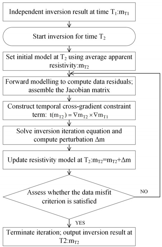
Figure 1.
Flowchart of the cross-gradient constrained time-lapse inversion at time T2.
Before a subsurface region underwent geological changes due to disturbances of actual construction or operation, this region exhibited resistivity distribution uniform in the reference model and spatial gradients small or even approaching zero. According to the construction method of the cross-gradient constraint term, the penalty imposed by the cross-gradient temporal constraint term remained small after the occurrence of real geological changes, regardless of the model resistivity changes in this region. Consequently, the model updating process was naturally dominated by the data residual term, and updating of resistivity in regions subjecting to real geological changes was encouraged. This mechanism allowed for imposing a weaker temporal constraint on the changed region without setting additional conditional functions, thus highlighting the true variations in resistivity.
3. Numerical Examples
3.1. Time-Lapse Resistivity
To verify the performance of the proposed time-lapse inversion method, numerical experiments with a pole-dipole acquisition configuration were conducted for two-dimensional resistivity monitoring. A total of 24 electrodes were set on the surface at equal spacing of 4 m. The survey line is 92 m long and centrally positioned. A resistivity model containing two time points (T1 and T2) was designed. The model is assumed to be isotropic and spatially homogeneous. Numerical test cases comprising a homogeneous background with geometrically regular anomaly bodies are a common benchmarking setup for validating resistivity inversion methods [36,46], enabling assessment of the inversion algorithm’s intrinsic imaging performance under controlled conditions.
Figure 2a illustrates the basic model at T1. This model featured a background resistivity of 100 Ω·m and a circular high-resistivity anomalous body with a resistivity of 500 Ω·m. The center of the anomalous body was located at x = 63 m and y = −13 m, with a radius of 6 m. The two-dimensional numerical model covers an area of 100 m × 30 m and is discretized into a uniform 100 × 30 rectangular grids, giving a total of 3000 cells. Figure 2b displays the time-lapse model at T2. In comparison to the basic model, this time-lapse model incorporated an additional identical circular high-resistivity anomalous body with a resistivity of 500 Ω·m. This additional anomalous body was positioned to the lower left of the first anomalous body and centered at x = 41 m and y = −16 m and also has a radius of 6 m. On account of these two resistivity models, synthetic data were generated using a forward modeling program based on the 2.5D finite element method. Random Gaussian white noise with an amplitude of 2% was then added to the synthetic apparent resistivity data.
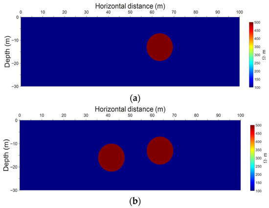
Figure 2.
Time-lapse resistivity models for two time points. (a) The basic model at T1. (b) The time-lapse model at T2.
3.2. Time-Lapse Inversion Results
Figure 3 presents the independent time-lapse inversion results at T1 and T2. Figure 3a shows the inversion results at T1, and Figure 3b presents the inversion results at T2. The initial inversion models were constructed using the average apparent resistivity data at corresponding times. The maximum number of inversion iterations was set to 10 uniformly.
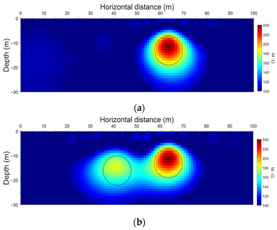
Figure 3.
Independent time-lapse inversion results at two time points. The black outline in the figure represents the actual anomalous regions with high resistivity. (a) Independent inversion result for the synthetic data of the basic model at T1 (RMS = 1.81%). (b) Independent inversion result for the synthetic data of the time-lapse model at T2 (RMS = 2.10%).
As seen in Figure 3a, the circular high-resistivity anomalous body in the upper right of the model could be clearly identified with the inversion results at T1. This anomalous body exhibited a morphology and position identical to the true model. However, its imaged morphology was slightly larger than the actual one due to the volume effect. As presented in Figure 3b, the two circular high-resistivity anomalous bodies could still be roughly identified with the inversion results at T2. Nevertheless, there were such issues as the volume effect and the non-uniqueness in inversion. The two anomalous bodies were connected notably in the inverted image, failing to accurately represent the two independent anomalous bodies in the true model. Although the ACB method was employed as the model constraint term in the independent inversion process to increase the spatial resolution of the inverted image, it was still hard to obtain accurate images depicting the temporal variations in resistivity. As such, the independent time-lapse inversion method is insufficient to reveal the change features of subsurface resistivity. To overcome the mentioned issues, it is necessary to introduce a constrained time-lapse inversion method.
To fully evaluate the performance of different constrained time-lapse inversion methods, this study employs different selection criteria for the time weighting matrix in Equation (3) as comparative experiments. If is selected as the product of a constant parameter and the roughness matrix of the model parameters, (3) corresponds to the constant constrained time-lapse inversion method [33]. If is a spatially varying cross-model constraint determined based on the temporal variation in the model parameters, (3) represents the time-lapse inversion method with spatially varying constraint [36]. This method can suppress the phenomenon of smooth resistivity distribution and highlight notable changes.
In addition, for the different constrained time-lapse inversion methods, a homogeneous model constructed from the mean apparent resistivity value was adopted as the initial model, and the synthetic data at T1 were independently inverted. The inversion result was completely consistent with Figure 3a. This inversion model was then utilized as both the initial model and reference model for the constrained time-lapse inversion at T2. On this basis, the T2 inversion results obtained with the different constrained time-lapse inversion methods are presented below.
Figure 4a provides the result of constant constrained time-lapse inversion. In this method, a uniform temporal constraint was imposed on all grid cells in the model to minimize the parameter differences between the prediction model and reference model. The constant temporal regularization parameter was set to1 × 10−3. The center of the high-resistivity anomalous body newly emerged in the lower left at T2 shifted upward slightly compared to the results obtained from the independent inversion. However, the constant temporal constraint was over-uniform, holding down the updating of genuine resistivity, resulting in excessively smooth imaging results of the anomalous body. This was specifically manifested as an upward deformation of the overall anomalous body, which deviated from the true model. Additionally, the constant constrained time-lapse inversion method did not resolve the issue of the connection between two anomalous bodies in independent inversion. The degree of differentiation between anomalous bodies remained insufficient.
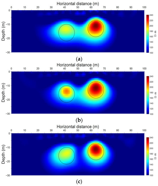
Figure 4.
Results of constrained time-lapse inversion. The black outline in the figure denotes the actual regions with anomalous resistivity. (a) Result of constant constrained time-lapse resistivity inversion at T2 (RMS = 1.97%). (b) Result of time-lapse resistivity inversion with spatially varying constraint at T2 (RMS = 2.17%). (c) Result of cross-gradient constrained time-lapse inversion at T2 (RMS = 2.45%).
Figure 4b presents the result of time-lapse inversion with spatially varying constraint. In this method, the intensity of temporal constraint was adjusted per the degree of the model’s parameter changes over time. Namely, weak constraints were applied to regions with significant changes, while strong constraints were imposed on regions with insignificant changes, thus yielding a more focused inversion image. The inversion result unveiled that the newly emerged high-resistivity anomalous body in the lower left showed a significant recovery in resistivity. The resistivity in its central region was notably higher than that obtained in other time-lapse inversion methods, hence validating the method’s ability to emphasize locally changed regions. However, there were certain drawbacks in the results of inversion with spatially varying constraint. Firstly, the morphology of the lower left anomalous body deviated from the true model. The true resistivity model consisted of two anomalous bodies of the same size. Yet, this feature was weakened in the inversion result but well represented in the independent time-lapse inversion result. In addition, the time-lapse inversion method with spatially varying constraint still failed to resolve the issue of the connection between two anomalous bodies. The independence between the anomalous bodies was still not fully reflected in the inversion result.
Figure 4c exhibits the result of cross-gradient constrained time-lapse inversion. In this method, the temporal constraint term minimized the difference in gradient directions between the inversion model at the current time and the reference model. This method highlighted genuine resistivity changes while maintaining structural consistency, yielding a more accurate distribution of subsurface resistivity. The constant regularization parameter in the cross-gradient constraint weighting matrix was set to 1 × 10⁻⁴. The objective function of this study contains only one constant regularization parameter for the cross-gradient structural constraint term, and its value directly affects the inversion quality. If this parameter is too small, the structural consistency constraint will be weakened, and the inversion result will be dominated by the data fitting term. If this parameter is too large, the structural constraint will be too strong, which will cause the inversion result to be over-smoothed and to mask the real changes. To determine the optimal value, this paper adopts the L-curve method [47]. In the L-curve diagram of the data fitting norm and the cross-gradient constraint norm, a significant inflection point can be identified. The corresponding optimal regularization parameter is 1 × 10⁻⁴, which achieves the best balance between data fitting and cross-gradient structural constraint. The L-curve is shown in Figure 5.
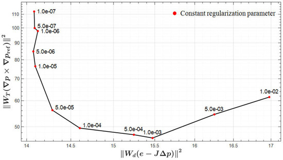
Figure 5.
L-curve of the data residual term versus the cross-gradient temporal constraint term. The constant regularization parameter was scanned over the range 1 × 10⁻⁷–1 × 10⁻².
Two distinct and independent high-resistivity anomalous bodies were shown in the inversion results, essentially eliminating the connection between anomalous bodies observed in previous methods. The boundaries of the anomalous bodies were sharper, and the overall geometrical morphology fitted the true model better than that obtained in other time-lapse inversion methods. Moreover, the inversion result did not exhibit excessive smoothing in the region with a newly emerged anomalous body due to the application of a temporal constraint term. This further validated the effectiveness of the cross-gradient temporal constraint term in automatically weakening the constraints in changed regions while strengthening the constraints in unchanged regions. The drawback of the inversion model overly converging towards the reference model was avoided effectively. This numerical result fully demonstrated that this inversion method could enhance the accuracy and spatial resolution of time-lapse inversion results. It was also capable of more accurately revealing the true spatiotemporal change features of subsurface resistivity and providing a more reliable imaging basis for the accurate interpretation of resistivity monitoring data.
The L-curve method has been successfully used in multiple field resistivity and time-lapse resistivity inversion studies to select the regularization parameter [18,48]. To systematically evaluate how the cross-gradient time constraint regularization parameter affects the imaging results, we conducted a one-order-of-magnitude sensitivity test around the L-curve corner at 1 × 10⁻⁴. Specifically, comparative inversions were run at 1 × 10⁻⁵ and 1 × 10⁻³, with all other settings held constant.
The inversion results are shown in Figure 6. As seen in Figure 6a, when the cross-gradient regularization parameter is decreased to 1 × 10⁻⁵, the structural-consistency constraint weakens and the solution becomes more data-driven. The two high-resistivity anomalies remain clearly separated, and the spacing between them is well preserved. However, relative to the 1 × 10⁻⁴ case, the peak amplitude at the center of the newly added left anomaly is slightly reduced, and the boundary contrast is slightly diminished. As shown in Figure 6b, when the cross-gradient regularization parameter is increased to 1 × 10⁻³, the structural-consistency constraint is markedly strengthened. The two high-resistivity anomalies remain separated, the intervening separation zone widens substantially, the boundary of the left anomaly becomes more diffuse, and its overall outline deviates slightly from the true circular shape.
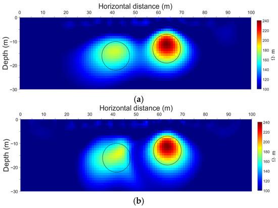
Figure 6.
Inversion results for different cross-gradient regularization parameters. The black outline in the figure denotes the actual regions with anomalous resistivity. (a) Inversion result with the cross-gradient regularization parameter set to 1 × 10⁻⁵. (b) Inversion result with the cross-gradient regularization parameter set to 1 × 10⁻³.
In this study, a normalized Mean Square Error (MSE) was introduced as an indicator to quantitatively assess the accuracy of the inversion models [38]. The purpose was to objectively evaluate the performance of different time-lapse inversion methods and quantitatively analyze the discrepancies between the inversion result and the true model. The MSE was calculated following the formula below:
where represents the time-lapse inversion model, and represents the true resistivity model. A smaller value of this indicator implies a smaller difference between the inversion result and the true model and higher accuracy in the inversion imaging result.
Only the normalized MSEs of the inversion results obtained at T2 were calculated and compared because all four methods at T1 adopted the same independent inversion process and resulted in identical models. The calculation results were summarized into a bar chart, as shown in Figure 7, to facilitate assessing the imaging accuracy of different time-lapse inversion strategies.
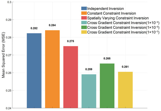
Figure 7.
Bar chart of MSEs for different time-lapse inversion methods.
In detail, the independent time-lapse inversion relied entirely on data fitting, lacking temporal prior. Thus, this inversion was susceptible to the volume effect of resistivity, leading to poor overall inversion accuracy, with a high MSE (0.282). This method was the baseline among the four methods. The constant constrained inversion method incorporated an additional temporal constraint term into the objective function. However, it imposed uniform penalties across the entire model, making it unable to distinguish between newly emerged anomalous bodies and stable regions. Consequently, it exhibited an excessive smoothing phenomenon, resulting in an MSE (0.284) slightly higher than that of the independent method. The time-lapse inversion method with spatially varying constraint weakened the penalties on significantly changed units, recovering the model updating for newly emerged anomalous bodies to some extent. As a result, this method had the MSE reduced to 0.275. In contrast, the cross-gradient constrained inversion method constrained the structural similarity between models, highlighting true resistivity changes and achieving the minimum error. When the cross-gradient regularization parameter is set to 1 × 10⁻⁵, 1 × 10⁻⁴, and 1 × 10⁻³, the MSEs are 0.265, 0.259, and 0.261, respectively. The L-curve–selected value of 1 × 10⁻⁴ yields the lowest MSE. The quantitative results of the MSE were highly consistent with the subjective judgment of the inversion images. This quantitative analysis further corroborated the comprehensive advantages of cross-gradient constraints in inhibiting the volume effect, maintaining structural consistency in time-lapse inversion, and highlighting true resistivity changes.
To quantitatively characterize the convergence behavior and data fit of the different inversion methods, we use the root-mean-square error (RMS), expressed as a percentage, as the evaluation metric and plot its evolution as an RMS (%) curve. RMS (%) is defined as the root mean square of the relative residuals between the observed and predicted data [42]. For observations, it is computed as:
RMS (%) directly reflects the magnitude of the relative error between observed and predicted data; its trajectory over iterations can be used to diagnose convergence and the level of fit. Figure 8 shows the RMS (%) curves at epoch T2 for the different inversion methods. In the case of the cross-gradient constrained time-lapse inversion, only the curve with a regularization parameter of 1 × 10⁻⁴ is shown, since the RMS (%) curves obtained with 1 × 10⁻³ and 1 × 10⁻⁵ differ only marginally. All curves exhibit a rapid initial decrease followed by a plateau and stabilize after 4–5 iterations, indicating good convergence across methods. In terms of the final RMS (%), the time-lapse inversion with a constant constraint is lowest (1.970%), followed by independent inversion (2.100%) and the time-lapse inversion with a spatially varying constraint (2.170%). The cross-gradient constrained time-lapse inversion yields similar values under the three regularization weights, 2.447% (1 × 10⁻⁵), 2.450% (1 × 10⁻⁴), and 2.456% (1 × 10⁻³), all slightly higher than the other methods. This indicates that introducing the cross-gradient time constraint into the objective function trades a slightly higher data misfit for stronger structural stability and boundary preservation, consistent with its improvement in the MSE metric.
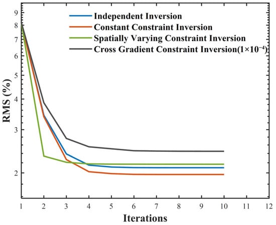
Figure 8.
RMS (%) curves at epoch T2 for different inversion methods.
To evaluate the impact of the cross-gradient time constraint on the time-lapse inversion results, we compute and present the cross-gradient field between each method’s inverted model and the reference model, thereby characterizing the spatial distribution of structural differences. Denote the model from a given inversion method as and the reference model as ; the cross-gradient field is calculated as:
We visualize the cross-gradient field, the visualization results are shown in Figure 9. On this basis, we adopt the L2 norm of the cross-gradient field as a quantitative metric, computed as:
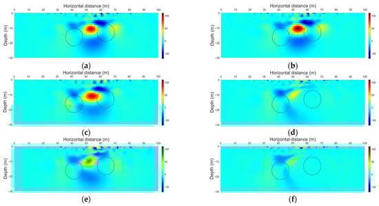
Figure 9.
Cross-gradient fields at epoch T2 for different inversion methods and their L2 norms. The black outline in the figure denotes the actual regions with anomalous resistivity. (a) Independent inversion, L2 norm = 650.29. (b) Constant constrained time-lapse resistivity inversion, L2 norm = 700.71; (c) Time-lapse resistivity inversion with spatially varying constraint, L2 norm = 663.59. (d) Cross-gradient constrained time-lapse inversion with regularization parameter 1 × 10⁻⁴, L2 norm = 362.78. (e) Cross-gradient constrained time-lapse inversion with regularization parameter 1 × 10⁻⁵, L2 norm = 461.15. (f) Cross-gradient constrained time-lapse inversion with regularization parameter 1 × 10⁻³, L2 norm = 293.43.
As shown in Figure 9, the three methods without the cross-gradient time constraint exhibit similar behavior in the cross-gradient field—broad spatial extent and larger magnitudes—and correspondingly high L2 norms: 650.29 for independent inversion, 700.71 for time-lapse inversion with a constant constraint, and 663.59 for time-lapse inversion with a spatially varying constraint. After introducing the cross-gradient time constraint, both the spatial extent and magnitude of the cross-gradient field decrease markedly. With the cross-gradient regularization parameter set to 1 × 10⁻⁴, the L2 norm drops to 362.78, and the map shows a clearly reduced spatial footprint and overall lower magnitudes. When the parameter is 1 × 10⁻⁵, the L2 norm rises to 461.15 and the overall distribution becomes more similar to that of the independent inversion. When the parameter is 1 × 10⁻³, the L2 norm further decreases to 293.43, with both the magnitude and spatial distribution reaching their minima. These results indicate that introducing the cross-gradient time constraint effectively suppresses structural inconsistency between models; moreover, the influence of the constraint becomes more pronounced as the regularization parameter increases.
To quantitatively compare computational efficiency across the inversion methods, we recorded the wall-clock time of the first iteration. All tests were conducted in a unified environment (MATLAB R2023b, Intel Core i7-12700H CPU, 16 GB RAM). The measured times were 23.21 s for the time-lapse independent inversion, 25.41 s for the time-lapse inversion with a constant constraint, 25.52 s for the time-lapse inversion with a spatially varying constraint, and 27.79 s for the cross-gradient constrained time-lapse inversion. The time differences arise mainly from the complexity of the constraint terms in the objective function. The time-lapse independent inversion includes only the data-misfit term and a model-smoothness regularization, so it has the smallest computational burden. The constant constraint and spatially varying constraint methods add model-difference-based temporal terms, which require additional matrix operations and therefore slightly increase runtime. The cross-gradient constrained method imposes a structural constraint that requires evaluation of the spatial gradient fields of the current and reference models and their cross product, as well as construction of the partial-derivative matrix of the cross-gradient functional with respect to the model parameters using a centered finite-difference scheme. These steps further increase computational cost. Given the improvements in inversion accuracy and resolution delivered by the cross-gradient constraint, this modest overhead is acceptable.
4. Physical Model Experiments
To validate the effectiveness of the proposed time-lapse inversion method, a rectangular concrete tank (internal dimension: 100 cm × 100 cm × 50 cm) was constructed based on numerical experiments. The experiment used a sand–cement mixture to construct a stable, controllable direct current conductive environment. Such sandbox/water-tank physical models are widely employed in resistivity methodological studies [49,50,51] to evaluate, under controlled conditions, the relative performance of data acquisition, inversion workflows, and constraint strategies. It should be noted that these analog materials cannot fully capture the complex electrical behavior of natural rock masses and may lead to optimistic estimates of imaging contrast in real geological media. The potential implications are analyzed further in Section 6.4 (Justification for the Simplified Medium Assumptions). The schematic diagram of the physical model structure is shown in Figure 10a, and the field physical model of the rectangular concrete tank is presented in Figure 10b. The inversion domain of the physical model was discretized into a 100 × 50 grid of cells, each measuring 1 cm × 1 cm. The model-filling medium was prepared by mixing sand and P.O 32.5 ordinary Portland cement at a 7:1 mass ratio.
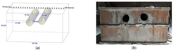
Figure 10.
Physical model experiment. (a) Schematic diagram of the physical model structure. The symbol ‘#’ is used to denote the electrode number. (b) Field physical model of the rectangular concrete tank.
In the experiments, temporal changes in subsurface resistivity were simulated by excavating cavities successively. The cavity positions were kept consistent with those in the numerical model. The upper right excavated cavity was centered at x = 63 cm, y = −13 cm, with a radius of 6 cm. The lower left excavated cavity was centered at x = 41 cm, y = −16 cm, also with a radius of 6 cm. After each cavity excavation, the mud was cleared away. The apparent resistivity data were collected after the cavity became dried. Specifically in the experiment, the upper right cavity was excavated first, followed by the measurement of apparent resistivity data. These apparent resistivity data were used as the observed data at T1. Subsequently, the lower left cavity was excavated, followed by the measurement of another set of apparent resistivity data. These apparent resistivity data were used as the observed data at T2. A total of 24 copper nails were used as observation electrodes, evenly spaced at an interval of 40 mm along the centerline of the tank’s top surface and perpendicular to the axial direction of the cavities. The survey line is 92 cm long and centrally positioned. This study used the YBD12 network-parallel direct current resistivity system for underground mining applications. The electrodes were small copper-pin electrodes. The source employed an alternating-polarity square wave. The current-injection duration was 0.5 s. The transmitter voltage was 24 V. The sampling interval was 50 ms. The apparent resistivity data were collected using a pole-dipole acquisition method. Given the great resistivity difference between the concrete matrix and air, all apparent resistivity data were logarithmically transformed using base 10 during data preprocessing. The logarithmic data were then uniformly adopted as input/output vectors for all inversion methods in the physical model experiments [36,38].
Under the T1 operating condition, the measured apparent resistivity data were first solved using the independent inversion strategy. The inversion result is displayed in Figure 11a. As an inversion result, a high-resistivity anomalous body located in the upper right of the tank was imaged clearly. Its spatial position was almost consistent with the coordinates of the actual cavity excavated at T1. Although there was some smearing at the boundaries of the high-resistivity zone, the overall morphology and size were recovered accurately. Therefore, this inversion model result was used as the initial and reference model for the constrained time-lapse inversion at T2.
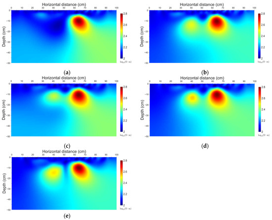
Figure 11.
(a) Result of independent time-lapse inversion at T1 (RMS = 5.13%). (b) Result of independent time-lapse inversion at T2 (RMS = 5.51%). (c) Result of constant constrained time-lapse inversion at T2 (RMS = 8.01%). (d) Result of time-lapse inversion with spatially varying constraint at T2 (RMS = 8.97%). (e) Result of cross-gradient constrained time-lapse inversion at T2 (RMS = 8.74%).
Under the T2 operating condition, the collected apparent resistivity data were solved using four different inversion strategies, separately. Figure 11b shows the result of independent time-lapse inversion. This method could image a newly excavated cavity in the lower left without incorporating any prior information. However, due to the non-uniqueness in inversion and the volume effect, the two high-resistivity anomalous bodies in the image appeared connected, failing to accurately manifest the two independent cavity structures in the physical model.
Figure 11c displays the result of the constant constrained time-lapse inversion method. In this method, the entire model was added with a uniform temporal smoothing term, establishing a temporal correlation with the reference model. Consequently, the imaging of the newly added cavity was more convergent than the independent inversion method. However, because of the temporal smoothing constraint, the newly excavated cavity in the lower left appeared to be slightly elevated. This inversion method suppressed some of the true resistivity changes, causing slight deviations in the overall morphology from the actual physical model.
Figure 11d presents the result of time-lapse inversion with spatially varying constraint. In this method, penalties in significantly changed regions were weakened, thereby boosting the response to the newly excavated cavity and resulting in a more focused inversion image in the lower left area. Yet, there were still connected artifacts between the two anomalous bodies, making it difficult to properly depict the independence between the two bodies.
In comparison, the cross-gradient constrained time-lapse inversion method (Figure 11e) fully leveraged the prior constraint for consistency in gradient directions. The boundaries of the high-resistivity anomalous bodies corresponding to the two cavities were clearly defined and separated from each other. The sizes and morphologies of the anomalous bodies in the inversion results closely matched those of the actual model, reconstructing the resistivity changes resulting from the two independent excavations in the time series. Figure 12 shows the RMS (%) curves at epoch T2 for different inversion methods. The independent inversion attains the lowest RMS (%), followed in order by the time-lapse inversion with a constant constraint, the cross-gradient constrained time-lapse inversion, and the time-lapse inversion with a spatially varying constraint. In addition, Figure 13 presents the cross-gradient fields at epoch T2 for the different methods together with their L2 norms.
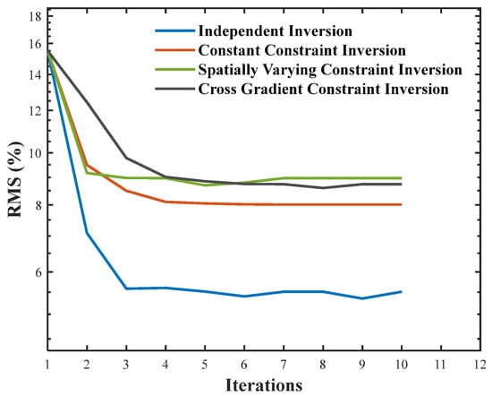
Figure 12.
RMS (%) curves at epoch T2 for different inversion methods.
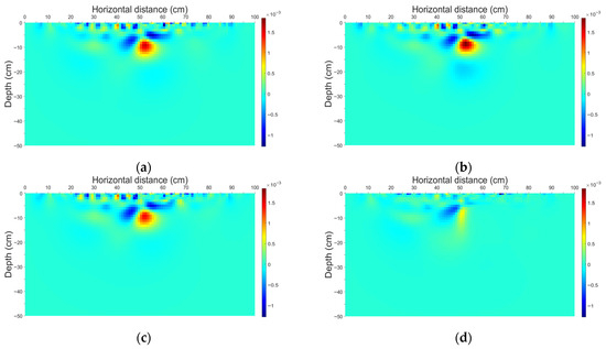
Figure 13.
Cross-gradient fields at epoch T2 for different inversion methods and their L2 norms. (a) Independent inversion, L2 norm = 0.0102; (b) Constant constrained time-lapse resistivity inversion, L2 norm = 0.0106; (c) Time-lapse resistivity inversion with spatially varying constraint, L2 norm = 0.0098; (d) Cross-gradient constrained time-lapse inversion, L2 norm = 0.0051.
Overall, the cross-gradient constraint not only maintained the structural consistency of the time-lapse inversion results but also greatly enhanced the resolution capability for local geological anomalies. The overall imaging accuracy of this inversion method surpassed those of the other three inversion methods, becoming more reliable for refined monitoring of dynamic geological changes.
5. Case Study
5.1. Background Information
Coal-bearing strata exhibit pronounced geological complexity. Superposed multi-phase tectonism has produced densely developed discontinuities with limited lateral continuity. In this context, concealed adverse geological bodies, such as blind faults and collapse columns, exhibit diverse spatial geometries and markedly variable connectivity. These factors collectively increase the uncertainty of underground engineering and the likelihood of hazard initiation. Under the disturbance induced by longwall retreat, the coal seam and its roof and floor strata undergo substantial stress redistribution. This redistribution drives the propagation and coalescence of pre-existing fractures and can reactivate concealed structures, thereby elevating geohazard risk. Accordingly, implementing continuous, quantitative monitoring of the coal-mining retreat process is of fundamental importance.
This study focuses on a coal mine in eastern China that employs strike longwall mining. The surrounding rock of the working face is dominated by sandstone and mudstone; the immediate roof consists of medium-grained sandstone, with a siltstone parting forming a false roof. The immediate floor comprises sandy mudstone and is underlain by sandstone constituting the main floor. A fault is present in the area, and a geological cross-section is shown in Figure 14. Mining-induced disturbance may trigger slip or shear failure along this fault, thereby altering its connectivity. Accordingly, we apply the direct current resistivity method in conjunction with time-lapse inversion to image signatures of fault reactivation during extraction.
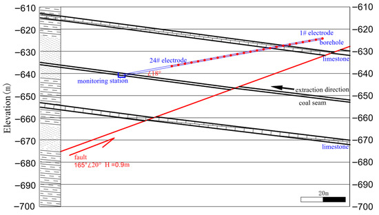
Figure 14.
Geological cross-section of the study area and layout of the monitoring and observation systems. The cross-section illustrates the stratigraphy and a fault (strike 165°, dip 20°, throw 0.9 m). The monitoring layout marks the locations of the monitoring station and the inclined monitoring borehole. Twenty-four electrodes (1#–24#, red dots) were installed in the borehole at 2.6 m spacing. The vertical axis indicates elevation (m), and the scale bar represents 20 m.
For monitoring the roof strata of a coal mine working face, an upward-inclined borehole is drilled along the strike within the face, equipped with electrode sensors to form a borehole direct current resistivity monitoring system. Subsequent inversion for a 2D/2.5D resistivity profile to characterize the electrical structure of the roof has been validated as a common and effective approach under the confined conditions of underground mines [52,53]. In implementation, an alcove within the panel roadway was selected to host a direct current resistivity monitoring station. A monitoring borehole (dip 18°, depth 91 m) was drilled in the alcove. After drilling, electrodes were installed and grouted to the surrounding rock to ensure adequate coupling. The survey line was 59.8 m long with 2.6 m electrode spacing; 24 electrodes were deployed, and apparent resistivity data were acquired using a pole–dipole array. This study used the YBD12 network-parallel direct current resistivity system for underground mining applications. The electrodes were stainless-steel electrodes. The source employed an alternating-polarity square wave. The current-injection duration was 0.5 s. The transmitter voltage was 96 V. The sampling interval was 50 ms. The layout of the monitoring borehole and observation system is shown in Figure 14. The volume between the survey line and the roof of the working face was defined as the target monitoring domain. Inversion employed a rectangular computational mesh with 1.3 m × 1.3 m cells. Two monitoring times were analyzed: D = 85 m (T1) and D = 75 m (T2), where D denotes the distance from the mining face to the monitoring station. Apparent resistivity datasets from both times were statistically summarized, as shown in Figure 15.
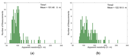
Figure 15.
Statistical distributions of apparent resistivity at two monitoring times. (a) T1 (D = 85 m), mean = 101.46 Ω·m. (b) T2 (D = 75 m), mean = 122.18 Ω·m.
5.2. Inversion Results
Time-lapse inversion was performed on the apparent resistivity observations acquired at two time points, D = 85 m (T1) and D = 75 m (T2). The T1 inversion result is shown in Figure 16a. The image reveals a high-resistivity anomaly near the deepest section of the monitoring borehole, which coincides with the limestone horizon in the study area and is consistent with the relatively higher resistivity of limestone compared with the adjacent strata. The T1 inversion model was then used as the reference model for the T2 inversion.
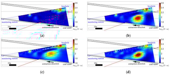
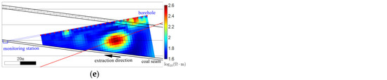
Figure 16.
Case study inversion results: (a) Independent inversion at T1 (RMS = 9.37%). (b) Independent inversion at T2 (RMS = 9.97%). (c) Constant constrained inversion at T2 (RMS = 11.44%). (d) Spatially varying constraint inversion at T2 (RMS = 10.62%). (e) Cross-gradient constraint inversion at T2 (RMS = 10.27%).
At T2, four inversion strategies were applied: independent inversion, constant constrained inversion, spatially varying constraint inversion, and cross-gradient constraint inversion. Figure 16b shows the independent inversion result. Figure 16c shows the constant constrained inversion result. Figure 16d shows the spatially varying constraint inversion result. Figure 16e shows the cross-gradient constraint inversion result. All results are plotted using a common color scale.
Within the monitored area, a fault has been exposed inside the working face. The fault zone is highly fractured and of low integrity, making it susceptible to stability problems under mining influence. In addition, during the retreat period no obvious or sustained water inflow or seepage was observed in the roof area of the working face within the direct current resistivity monitoring footprint. At epoch T2, all inversion results in Figure 16b–e reveal a newly emergent high-resistivity anomaly near the fault. In plan view the anomaly is approximately elliptical; its center coincides with the mapped fault trace, and its major axis is roughly parallel to the fault strike. This pronounced spatial correspondence indicates that the anomaly is closely related to fault activity.
During retreat, the in-panel fault may experience fracture dilation, shear slip, caving of the goaf (mined-out area), and local water ingress or escape. These processes modify pore structure, fracture connectivity, and saturation, thereby changing resistivity. Given the absence of conspicuous inflow and the spatial characteristics of the high-resistivity anomaly, we interpret the newly observed high-resistivity body at T2 as fault-fracture opening caused by mining-induced stress redistribution. Fracture dilation permits air ingress; because air has extremely high resistivity, its presence provides a direct physical cause of the strong high-resistivity response. It should be noted that inferring geological processes from resistivity inversion alone carries uncertainty, and the observed anomaly may reflect multiple mechanisms acting together. The above interpretation for the T2 high-resistivity anomaly should therefore be regarded as a reasoned inference rather than a definitive conclusion.
Specifically, in the independent inversion the volume effect causes partial spatial linkage between the new high resistivity anomaly and the limestone high resistivity zone. In the constant constrained inversion the new high resistivity anomaly remains discernible. Its peak amplitude is lower than in the independent inversion. Its centroid shifts slightly upward. Its outer margin expands moderately and the boundary becomes smoother. The local linkage to the limestone high resistivity zone becomes more pronounced. In the spatially varying constraint inversion, the anomaly’s central position is essentially stable. Its peak resistivity exceeds that of the independent inversion and the core becomes more focused. The local linkage to the limestone zone is still identifiable but weaker, and the background limestone high resistivity band is more diffuse relative to the reference model. In the cross-gradient constraint inversion the anomaly’s peak amplitude is also slightly higher than in the independent inversion and its boundary becomes slightly more compact. The previous local linkage to the limestone high resistivity zone is no longer evident, and the anomaly appears as a relatively independent high resistivity body. Figure 17 depicts the RMS (%) curves for the different inversion methods. Figure 18 shows the spatial distribution of the cross-gradient fields for the different methods together with the corresponding L2 norms.
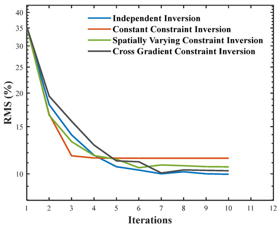
Figure 17.
RMS (%) curves at epoch T2 for different inversion methods.
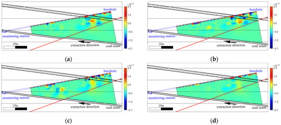
Figure 18.
Cross-gradient fields at epoch T2 for different inversion methods and their L2 norms. (a) Independent inversion, L2 norm = 0.0073; (b) Constant constrained time-lapse resistivity inversion, L2 norm = 0.0084; (c) Time-lapse resistivity inversion with spatially varying constraint, L2 norm = 0.0085; (d) Cross-gradient constrained time-lapse inversion, L2 norm = 0.0056.
Taken together, all methods consistently image a near elliptical high resistivity anomaly in the vicinity of the fault, with its major axis approximately aligned with the fault strike. In comparison, the spatially varying constraint inversion yields the highest peak at the anomaly center and produces a more focused core region. The cross-gradient constraint inversion performs better in structural delineation, clearly defining the boundary between the new high resistivity anomaly near the fault and the pre-existing limestone high resistivity zone. The overall image presents these as mutually independent high resistivity units, making this approach better suited to monitoring scenarios dominated by discontinuous changes.
6. Discussion
6.1. Scenario Applicability of the Method
This method is primarily tailored to monitoring dynamic geological models that un-dergo discontinuous changes. Its applicability may therefore be restricted when the target evolves through progressive, gradual expansion of an existing structure, such as the slow migration of a tracer plume. Future research will focus on enhancing the method so that it can accommodate monitoring scenarios characterized by continuous, smoothly evolving changes.
6.2. Cross-Gradient and 4D Inversion
This study proposes and validates a new temporal constraint strategy, the cross-gradient time constraint, evaluated within a constrained time-lapse inversion framework. It is important to emphasize that, in principle, this strategy does not depend on a specific inversion framework and can be directly embedded in a 4D inversion framework.
The 4D inversion framework is an important route for time-lapse imaging. It incorporates the full time series of data and models into a single objective function and solves them simultaneously. In monitoring scenarios with many epochs and continuously evolving media, this approach exploits temporal information more fully, enhances overall temporal consistency and noise robustness, and has demonstrated strong stability across a variety of applications [24,39]. By contrast, the constrained time-lapse inversion framework solves the problem epoch by epoch, providing a more direct solution path with a lower computational burden [48]. Given that our dataset contains only two epochs and the changes are localized and abrupt, the potential advantages of the 4D framework cannot be fully realized in this case. Moreover, the 4D framework entails strong space–time coupling and higher algorithmic complexity [54]. Therefore, at this stage we adopt the constrained time-lapse inversion framework for validation, which helps attribute improvements in the inversion results specifically to the temporal constraint strategy itself [55].
When the number of epochs is limited (for example, only two epochs in this study), the difference in imaging performance between the constrained time-lapse inversion framework and the 4D inversion framework is not pronounced, and the advantage of integrating the full time series in 4D is not fully realized [24]. Moreover, many existing 4D inversion methods employ model-difference-based temporal constraints. Although such constraints are effective in suppressing nonphysical temporal oscillations, fixed weights can adversely affect localized abrupt changes, leading to amplitude attenuation and boundary blurring. Our experimental results corroborate this limitation.
To address these shortcomings, prior studies have proposed active time constraint (ATC) and related spatiotemporally adaptive weighting schemes to increase sensitivity to localized genuine changes. These approaches update the temporal weights based on change indicators (often the model update) and apply spatial diffusion rules, and the imaging outcome can be highly sensitive to the associated parameters. Inappropriate parameter choices may cause non-geological over-focusing and mislead geological interpretation [40].
Unlike model-difference-based temporal constraints, the cross-gradient time constraint introduced here penalizes directional inconsistency in the model gradients between epochs rather than directly penalizing amplitude differences. It is therefore better suited to emphasizing true local changes while preserving sharp boundaries. We select the regularization parameter using the L-curve method, which reduces reliance on ad hoc thresholds and scheduling rules. In both the numerical and the physical-model experiments in this study, this constraint did not produce obvious over-smoothing and showed advantages in boundary delineation.
Future work will embed the cross-gradient time constraint within a 4D inversion framework and perform systematic, head-to-head comparisons with representative methods to evaluate its applicability in that framework and to assess its advantages and potential limitations relative to other 4D approaches.
6.3. 2.5D Approximation and 3D Effects
This study performs inversion imaging under scenarios with inherently three-dimensional characteristics using a 2.5D framework. Given that dimensionality reduction may introduce systematic bias, this issue warrants a systematic discussion.
In this work, the 2.5D inversion is implemented on a 2D mesh while incorporating the three-dimensional point-source effect via spectral integration over strike wavenumbers, under the premise that the electrical structure is invariant along strike. Consequently, it better approximates the true 3D response than conventional 2D inversion. When out-of-section anomalies have finite along-strike extent, 2D imaging is prone to pronounced 3D effects that can produce projection artifacts and related issues [43,56]. Under identical acquisition conditions, introducing 2.5D can partially mitigate these distortions. Considering computational cost, 2.5D inversion is also well-suited to long profiles, single-line acquisitions, and multi-epoch time-lapse applications [57].
By contrast, 3D inversion discretizes the subsurface in three dimensions and does not rely on the assumption of along-strike uniformity, thereby allowing electrical variations in all directions to be accounted for simultaneously and yielding a more complete representation of the true 3D structure. Accordingly, when multiple survey lines are available within the study area, 3D inversion is preferable.
In our field site, the monitoring area lies in a confined underground environment. Limitations imposed by the roadway cross-section, borehole construction, and electrode deployment precluded multi-line layouts or a full 3D acquisition. Under the practical constraint of having only a single survey line along strike, adopting 2.5D inversion is therefore a reasonable and feasible engineering choice [52]. The proposed cross-gradient time constraint is a form of regularization that aims to preserve structural consistency between adjacent epochs while highlighting differences caused by genuine geological change. This strategy is intrinsically independent of the spatial dimensionality and discretization of the forward operator; it depends only on computing the model gradient field. In spaces of different dimensionality, the gradient operator is defined accordingly. Hence, the method is readily extensible to 3D inversion.
To further verify the robustness of the proposed cross-gradient time constraint under truly 3D conditions, future work will focus on inversion studies using 3D synthetic experiments.
6.4. Justification for the Simplified Medium Assumptions
This study adopts simplified assumptions in both the numerical simulations and the physical-tank experiment to benchmark the method under controlled conditions. In the simulations, we use a homogeneous, isotropic background with geometrically regular anomalies; in the physical experiment, we employ a sand-cement analog. These controlled and comparable settings allow us to test the imaging performance of the cross-gradient constrained time-lapse inversion, which is a common and reasonable practice in geophysical inversion studies.
Nevertheless, it must be recognized that such simplifications depart systematically from real subsurface media, which affects the transferability of our conclusions to engineering applications. First, natural formations typically exhibit electrical heterogeneity and anisotropy, which alter current-flow patterns and cause the observations to reflect a complex composite response. Under these conditions, inversions predicated on homogeneity and isotropy may introduce imaging bias and reduce interpretational reliability [58]. In addition, our analysis is based on a direct current resistivity assumption and does not account for induced polarization (IP). In clay-rich and mineralized strata, conduction mechanisms are more complex, involving surface conduction and spectral induced polarization (SIP), which leads to frequency-dependent effective resistivity [59]. This implies an inherent non-uniqueness in apparent-resistivity variations: direct current measurements alone cannot discriminate between structural changes and polarization effects, risking misattribution of the latter as the former.
Despite these limitations, the overall strategy of enforcing structural consistency to enhance the resolution of multi-epoch imaging and suppress artifacts remains effective. Future work will focus on developing an inversion framework that incorporates an anisotropic resistivity tensor and on constructing high-fidelity models with heterogeneous backgrounds to more realistically simulate current-flow distributions. To address non-uniqueness, we will also explore joint inversion of resistivity and IP parameters. These efforts aim to delineate the method’s applicability bounds under complex geological conditions and to provide a more robust basis for engineering deployment.
6.5. Noise Effects and Method Applicability
In the numerical simulations described above, we first superimposed 2% Gaussian random noise on the observations to test the method’s robustness under noisy conditions, a practice that is common in resistivity inversion studies. However, field noise often departs from a purely Gaussian distribution; in addition to instrument precision and electrode contact resistance, it may include finite-amplitude systematic perturbations or non-Gaussian disturbances. To better approximate field conditions, we therefore added an additional 4% random noise on top of the 2% Gaussian noise, so as to capture the coexistence of Gaussian fluctuations and finite-amplitude random disturbances in real data. The noise-contaminated data were then used in the time-lapse inversion analyses presented here. The inversion results for the different methods are shown in Figure 19.
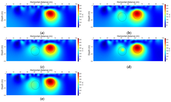
Figure 19.
Inversion results under 2% Gaussian random noise plus an additional 4% random noise. The black outline in the figure denotes the actual regions with anomalous resistivity. (a) Time-lapse independent inversion at epoch T1. (b) Time-lapse independent inversion at epoch T2. (c) Constant constrained time-lapse resistivity inversion at epoch T2. (d) Time-lapse resistivity inversion with spatially varying constraint at epoch T2. (e) Cross-gradient constrained time-lapse inversion at epoch T2.
Under the 2% Gaussian noise plus 4% random noise setting, all time-lapse inversions are affected to varying degrees, with common symptoms including increased artifacts, blurred boundaries, and shape shifts. Specifically, Figure 19b shows that the newly introduced high-resistivity anomaly has a weaker amplitude, diffuse boundaries, and a slight overall upward shift; volumetric smearing produces a tendency for local connectivity between the two high-resistivity zones. In Figure 19c, the new high-resistivity anomaly is more focused than in 19b and the connectivity artifact is reduced, but the model-difference time constraint makes the upward shift more pronounced. In Figure 19d, the anomaly’s central amplitude increases and the peak position lies slightly above the true center; the overall morphology is displaced and elongated toward the upper left, deviating from the true circular outline, and the separation between the two anomalies remains limited. In Figure 19e, two high-resistivity anomalies are clearly separated and the connectivity artifact is largely eliminated. Although the equal-sized features cannot be fully reconstructed under the noise contamination, the degree of recovery is markedly better than with the other methods, and the morphology and structural consistency more closely resemble the true model.
Under this noise setting, we evaluate the MSE at epoch T2 for each inversion method: time-lapse independent inversion, MSE = 0.3212; time-lapse inversion with a constant constraint, MSE = 0.3230; time-lapse inversion with a spatially varying constraint, MSE = 0.3202; and cross-gradient constrained time-lapse inversion, MSE = 0.3046.
In addition, Figure 20 presents the RMS (%) curves for the different inversion methods. Figure 21 also shows the spatial distribution of the cross-gradient fields for the different methods together with the corresponding L2 norms.
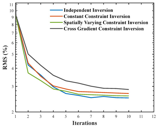
Figure 20.
RMS (%) curves at epoch T2 for different inversion methods.
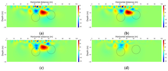
Figure 21.
Spatial distribution of the cross-gradient fields for different inversion methods and their corresponding L2 norms. The black outline in the figure denotes the actual regions with anomalous resistivity. (a) Independent inversion (L2 norm = 446.11). (b) Constant constrained time-lapse resistivity inversion (L2 norm = 459.31). (c) Time-lapse resistivity inversion with spatially varying constraint (L2 norm = 439.68). (d) Cross-gradient constrained time-lapse inversion (L2 norm = 228.25).
7. Conclusions
(1) A cross-gradient constrained time-lapse resistivity inversion method is proposed, in which a cross-gradient term is integrated into the constrained time-lapse inversion framework to enforce structural similarity between the inversion model and a reference model. By promoting updates attributable to genuine geological changes while preserving structural consistency across epochs, the method reliably depicts temporal variations in subsurface resistivity and accurately captures time-varying features. Consequently, the approach improves imaging fidelity and provides a novel structural prior for resistivity monitoring, with strong applicability to long-term monitoring and the identification of dynamic geological changes.
(2) Numerical simulations and similar physical model experiments were conducted to thoroughly validate the imaging performance of the proposed method. Compared with traditional time-lapse inversion methods, the proposed method could consistently produce images that most aligned with the subsurface resistivity changes. In synthetic tests, the proposed method preserved the geometric structure of anomalous bodies and reduced the normalized MSE, markedly improving the accuracy and resolution of the inversion results. The physical tank experiments also demonstrated that the proposed method exhibited notable advantages in reconstructing given subsurface features, showcasing its potential in time-lapse imaging for high-resolution monitoring. Finally, the method was applied to a case study monitoring fault activation under coalface retreat conditions; the results clearly delineated the boundary between the newly developed high-resistivity anomaly in the fault neighborhood and the pre-existing high-resistivity limestone belt, further demonstrating its practical effectiveness.
Author Contributions
Conceptualization, S.C. and B.W.; methodology, S.C.; software, S.C.; validation, S.C., B.W. and H.Y.; formal analysis, S.C. and H.Y.; investigation, S.C.; resources, B.W. and H.Y.; data curation, B.W.; writing—original draft preparation, S.C.; writing—review and editing, B.W.; visualization, S.C.; supervision, B.W. and H.Y.; project administration, B.W. and Y.L.; funding acquisition, B.W. and Y.L. All authors have read and agreed to the published version of the manuscript.
Funding
This research was supported in part by the Deep Earth Probe and Mineral Resources Exploration-National Science and Technology Major Project (2024ZD1004103), in part by the National Natural Science Foundation of China (No. 42174165, No. 42404148), and in part by the Natural Science Foundation of Jiangsu Province (No. BK20230197).
Data Availability Statement
The data presented in this study are available on request from the corresponding author.
Conflicts of Interest
All authors declare that this study was conducted without any commercial or financial relationships that could be perceived as a potential conflict of interest.
References
- Wang, J.; Zhang, S.; Lv, T.-K.; Liu, Y.; Ji, K.-P. Method application of distributed optical fiber Brillouin sensing in slope monitoring. In Proceedings of the IEEE 6th Advanced Information Management, Communication, Electronic and Automation Control Conference (IMCEC), Chongqing, China, 24–26 May 2024. [Google Scholar]
- Wang, B.; Liu, S.-D.; Li, S.-N.; Zhou, F.-B. Double-transmitting and sextuple-receiving borehole transient electromagnetic method and experimental study. Earth Sci. Res. J. 2017, 21, 77–83. [Google Scholar] [CrossRef]
- Farmani, M.B.; Kitterød, N.-O.; Keers, H. Inverse modeling of unsaturated flow parameters using dynamic geological structure conditioned by GPR tomography. Water Resour. Res. 2008, 44, W08401. [Google Scholar] [CrossRef]
- Wang, B.; Jin, B.; Huang, L.-Y.; Liu, S.-D.; Sun, H.-C.; Liu, J.-C.; Ding, X.; Wang, S.-C. A Hilbert polarization imaging method with breakpoint diffracted wave in front of roadway. J. Appl. Geophys. 2020, 177, 104032. [Google Scholar] [CrossRef]
- Whiteley, J.-S.; Chambers, J.-E.; Uhlemann, S.; Wilkinson, P.-B.; Kendall, J.-M. Geophysical monitoring of moisture-induced landslides: A review. Rev. Geophys. 2019, 57, 106–145. [Google Scholar] [CrossRef]
- Slater, L.; Binley, A. Advancing hydrological process understanding from long-term resistivity monitoring systems. WIREs Water 2021, 8, e1513. [Google Scholar] [CrossRef]
- Massarweh, O.; Abushaikha, A.S. CO2 sequestration in subsurface geological formations: A review of trapping mechanisms and monitoring techniques. Earth-Sci. Rev. 2024, 253, 104793. [Google Scholar] [CrossRef]
- Lu, T.; Liu, S.-D.; Wang, B.; Wu, R.-X.; Hu, X.-W. A review of geophysical exploration technology for mine water disaster in China: Applications and trends. Mine Water Environ. 2017, 36, 331–340. [Google Scholar] [CrossRef]
- Barker, R.; Moore, J. The application of time-lapse electrical tomography in groundwater studies. Lead. Edge 1998, 17, 1454–1458. [Google Scholar] [CrossRef]
- Chang, P.-Y.; Chang, L.-C.; Hsu, S.-Y.; Tsai, J.-P.; Chen, W.-F. Estimating the hydrogeological parameters of an unconfined aquifer with the time-lapse resistivity-imaging method during pumping tests: Case studies at the Pengtsuo and Dajou sites, Taiwan. J. Appl. Geophys. 2017, 144, 134–143. [Google Scholar] [CrossRef]
- Thompson, J.; Buda, A.; Shober, A.; Ntarlagiannis, D.; Collick, A.; Kennedy, C.; Mosesso, L.; Reiner, M.; Triantafilis, J.; Pokhrel, S.; et al. Electrical geophysical monitoring of subsurface solute transport in low-relief agricultural landscapes in response to a simulated major rainfall event. J. Hydrol. 2025, 646, 132313. [Google Scholar] [CrossRef]
- Daily, W.; Ramirez, A. Electrical resistance tomography during in-situ trichloroethylene remediation at the Savannah River Site. J. Appl. Geophys. 1995, 33, 239–249. [Google Scholar] [CrossRef]
- Ugbor, C.C.; Ikwuagwu, I.E.; Ogboke, O.J. 2D inversion of electrical resistivity investigation of contaminant plume around a dumpsite near Onitsha expressway in southeastern Nigeria. Sci. Rep. 2021, 11, 11854. [Google Scholar] [CrossRef]
- Nivorlis, A.; Rossi, M.; Dahlin, T. Temporal filtering and time-lapse inversion of geoelectrical data for long-term monitoring with application to a chlorinated hydrocarbon contaminated site. Geophys. J. Int. 2022, 228, 1648–1664. [Google Scholar] [CrossRef]
- Wilkinson, P.; Chambers, J.; Uhlemann, S.; Meldrum, P.; Smith, A.; Dixon, N.; Loke, M.H. Reconstruction of landslide movements by inversion of 4-D electrical resistivity tomography monitoring data. Geophys. Res. Lett. 2016, 43, 1166–1174. [Google Scholar] [CrossRef]
- Palis, E.; Lebourg, T.; Vidal, M.; Levy, C.; Tric, E.; Hernandez, M. Multiyear time-lapse ERT to study short- and long-term landslide hydrological dynamics. Landslides 2017, 14, 1333–1343. [Google Scholar] [CrossRef]
- Lapenna, V.; Perrone, A. Time-lapse electrical resistivity tomography (TL-ERT) for landslide monitoring: Recent advances and future directions. Appl. Sci. 2022, 12, 1425. [Google Scholar] [CrossRef]
- Bergmann, P.; Schmidt-Hattenberger, C.; Kiessling, D.; Rücker, C.; Labitzke, T.; Henninges, J.; Baumann, G.; Schütt, H. Surface-downhole electrical resistivity tomography applied to monitoring of CO2 storage at Ketzin, Germany. Geophysics 2012, 77, B253–B267. [Google Scholar]
- Bergmann, P.; Ivandic, M.; Norden, B.; Rücker, C.; Kiessling, D.; Lüth, S.; Schmidt-Hattenberger, C.; Juhlin, C. Combination of seismic reflection and constrained resistivity inversion with an application to 4D imaging of the CO2 storage site, Ketzin, Germany. Geophysics 2014, 79, B37–B50. [Google Scholar] [CrossRef]
- Khan, S.; Khulief, Y.; Juanes, R.; Bashmal, S.; Usman, M.; Al-Shuhail, A. Geomechanical modeling of CO2 sequestration: A review focused on CO2 injection and monitoring. J. Environ. Chem. Eng. 2024, 12, 112847. [Google Scholar] [CrossRef]
- Liu, S.-C.; Liu, X.-M.; Jiang, Z.-H.; Xing, T.; Chen, M.-Z. Research on electrical prediction for evaluating water conducting fracture zones in coal seam floor. Chin. J. Rock Mech. Eng. 2009, 28, 348–356. [Google Scholar]
- Jin, D.-W.; Zhao, C.-H.; Duan, J.-H.; Qiao, W.; Lu, J.-J.; Li, P.; Zhou, Z.-F.; Li, D.-S. Research on 3D monitoring and intelligent early warning system for water hazard of coal seam floor. J. China Coal Soc. 2020, 45, 2256–2264. [Google Scholar]
- Yang, H.; Liu, S.; Yang, C. Dynamic monitoring of mining destruction on coal seam floor with constrained time-lapse resistivity imaging inversion. IEEE Access 2022, 10, 84799–84808. [Google Scholar] [CrossRef]
- Hayley, K.; Pidlisecky, A.; Bentley, L.R. Simultaneous time-lapse electrical resistivity inversion. J. Appl. Geophys. 2011, 75, 401–411. [Google Scholar] [CrossRef]
- Liu, J.-C.; Zhang, Z.-Y.; Zhou, F.; Li, M.; Ou, Y.-W.; Yang, L.; Yi, K. Two-dimensional joint inversion of DC resistivity method and seismic traveltime tomography method based on the FCM cluster constraint. Chin. J. Geophys. 2023, 66, 3048–3059. [Google Scholar]
- Tao, T.; Han, P.; Ma, H.; Tan, H.-D. 3D time-lapse resistivity inversion. Chin. J. Geophys. 2024, 67, 3973–3988. [Google Scholar]
- Cho, I.-K.; Jeong, D.-B. 4D inversion of resistivity monitoring data with adaptive time domain regularization. J. Appl. Geophys. 2022, 198, 104559. [Google Scholar] [CrossRef]
- De Franco, R.; Biella, G.; Tosi, L.; Teatini, P.; Lozej, A.; Chiozzotto, B.; Giada, M.; Rizzetto, F.; Claude, C.; Mayer, A.; et al. Monitoring the saltwater intrusion by time-lapse electrical resistivity tomography: The Chioggia test site (Venice Lagoon, Italy). J. Appl. Geophys. 2009, 69, 117–130. [Google Scholar] [CrossRef]
- Inim, I.J.; Udosen, N.I.; Tijani, M.N.; Affiah, U.E.; George, N.J. Time-lapse electrical resistivity investigation of seawater intrusion in coastal aquifer of Ibeno, Southeastern Nigeria. Appl. Water Sci. 2020, 10, 1–12. [Google Scholar] [CrossRef]
- Daily, W.; Ramirez, A.; LaBrecque, D.; Nitao, J. Electrical resistivity tomography of vadose water movement. Water Resour. Res. 1992, 28, 1429–1442. [Google Scholar] [CrossRef]
- Liu, B.; Liu, Z.-Y.; Li, S.-C.; Fan, K.-R.; Nie, L.-C.; Zhang, X.-X. An improved time-lapse resistivity tomography to monitor and estimate the impact on the groundwater system induced by tunnel excavation. Tunn. Undergr. Space Technol. 2017, 66, 107–120. [Google Scholar] [CrossRef]
- LaBrecque, D.; Alumbaugh, D.L.; Yang, X.-J.; Paprocki, L.; Brainard, J. Three-dimensional monitoring of vadose zone infiltration using electrical resistivity tomography and cross-borehole ground-penetrating radar. Methods Geochem. Geophys. 2002, 35, 259–272. [Google Scholar]
- Loke, M.H. Constrained time-lapse resistivity imaging inversion. In Proceedings of the Symposium on the Application of Geophysics to Engineering and Environmental Problems (SAGEEP), Denver, CO, USA, 14–19 March 2001. [Google Scholar]
- Oldenborger, G.A.; Knoll, M.D.; Routh, P.S.; LaBrecque, D.J. Time-lapse ERT monitoring of an injection/withdrawal experiment in a shallow unconfined aquifer. Geophysics 2007, 72, F177–F187. [Google Scholar] [CrossRef]
- Miller, C.R.; Routh, P.S.; Brosten, T.R.; McNamara, J.P. Application of time-lapse ERT imaging to watershed characterization. Geophysics 2008, 73, G7–G17. [Google Scholar] [CrossRef]
- Kim, K.-J.; Cho, I.-K. Time-lapse inversion of 2D resistivity monitoring data with a spatially varying cross-model constraint. J. Appl. Geophys. 2011, 74, 114–122. [Google Scholar] [CrossRef]
- Fiandaca, G.; Doetsch, J.; Vignoli, G.; Auken, E. Generalized focusing of time-lapse changes with applications to direct current and time-domain induced polarization inversions. Geophys. J. Int. 2015, 203, 1101–1112. [Google Scholar] [CrossRef]
- Hermans, T.; Kemna, A.; Nguyen, F. Covariance-constrained difference inversion of time-lapse electrical resistivity tomography data. Geophysics 2016, 81, E311–E322. [Google Scholar] [CrossRef]
- Kim, J.-H.; Yi, M.-J.; Park, S.-G.; Kim, J.G. 4-D inversion of DC resistivity monitoring data acquired over a dynamically changing earth model. J. Appl. Geophys. 2009, 68, 522–532. [Google Scholar] [CrossRef]
- Karaoulis, M.C.; Kim, J.-H.; Tsourlos, P.I. 4D active time constrained resistivity inversion. J. Appl. Geophys. 2011, 73, 25–34. [Google Scholar] [CrossRef]
- Karaoulis, M.; Tsourlos, P.; Kim, J.-H.; Revil, A. 4D time-lapse ERT inversion: Introducing combined time and space constraints. Near Surf. Geophys. 2014, 12, 25–34. [Google Scholar] [CrossRef]
- Loke, M.H.; Barker, R.D. Least-squares deconvolution of apparent resistivity pseudosections. Geophysics 1995, 60, 1682–1690. [Google Scholar] [CrossRef]
- Sjödahl, P.; Dahlin, T.; Zhou, B. 2.5 D resistivity modeling of embankment dams to assess influence from geometry and material properties. Geophysics 2006, 71, G107–G114. [Google Scholar] [CrossRef]
- Yi, M.-J.; Kim, J.-H.; Chung, S.-H. Enhancing the resolving power of least-squares inversion with active constraint balancing. Geophysics 2003, 68, 931–941. [Google Scholar] [CrossRef]
- Loke, M.H.; Lane, J.W. The use of constraints in 2D and 3D resistivity modelling. In Proceedings of the 8th Environmental and Engineering Geophysical Society European Section (EEGS-ES) Meeting, Aveiro, Portugal, 21–25 October 2002. [Google Scholar]
- Jaysaval, P.; Hammond, G.E.; Johnson, T.C. Massively parallel modeling and inversion of electrical resistivity tomography data using PFLOTRAN. Geosci. Model Dev. Discuss. 2022, 2022, 1–26. [Google Scholar] [CrossRef]
- Hansen, P.C. Analysis of discrete ill-posed problems by means of the L-curve. SIAM Rev. 1992, 34, 561–580. [Google Scholar] [CrossRef]
- Loke, M.H.; Dahlin, T.; Rucker, D.F. Smoothness-constrained time-lapse inversion of data from 3D resistivity surveys. Near Surf. Geophys. 2014, 12, 5–24. [Google Scholar] [CrossRef]
- Pollock, D.; Cirpka, O.A. Fully coupled hydrogeophysical inversion of a laboratory salt tracer experiment monitored by electrical resistivity tomography. Water Resour. Res. 2012, 48, W01505. [Google Scholar] [CrossRef]
- Singha, K.; Day-Lewis, F.D.; Johnson, T.; Slater, L.D. Advances in interpretation of subsurface processes with time-lapse electrical imaging. Hydrol. Process. 2015, 29, 1549–1576. [Google Scholar] [CrossRef]
- Adepelumi, A.A.; Solanke, A.A.; Sanusi, O.B.; Shallangwa, A.M. Model tank electrical resistivity characterization of LNAPL migration in a clayey-sand formation. Environ. Geol. 2006, 50, 1221–1233. [Google Scholar] [CrossRef]
- Wu, R.-X.; Wu, Y.-Z.; Sun, B.-Y.; Zhou, G.-Q.; Zheng, L.-L. Monitoring of Overburden Failure with a Large Fractured-Height Working Face in a Deep Jurassic Coal Seam Based on the Electric Method. Appl. Sci. 2024, 14, 10293. [Google Scholar] [CrossRef]
- Du, L.; Zhu, W.-J.; Wang, L.; Li, H.; Jiao, X.-Y.; Qin, T. Using roof borehole electrical resistivity tomography to monitor roof water infiltration in a mine work face. Sci. Rep. 2025, 15, 2621. [Google Scholar] [CrossRef]
- Dimech, A.; Cheng, L.-Z.; Chouteau, M.; Chambers, J.; Uhlemann, S.; Wilkinson, P.; Meldrum, P.; Mary, B.; Fabien-Ouellet, G.; Isabelle, A. A review on applications of time-lapse electrical resistivity tomography over the last 30 years: Perspectives for mining waste monitoring. Surv. Geophys. 2022, 43, 1699–1759. [Google Scholar] [CrossRef] [PubMed]
- Kim, J.-H.; Supper, R.; Tsourlos, P.; Yi, M.-J. Four-dimensional inversion of resistivity monitoring data through Lp norm minimizations. Geophys. J. Int. 2013, 195, 1640–1656. [Google Scholar] [CrossRef]
- Bai, P.; Vignoli, G.; Hansen, T.M. 1D stochastic inversion of airborne time-domain electromagnetic data with realistic prior and accounting for the forward modeling error. Remote Sens. 2021, 13, 3881. [Google Scholar] [CrossRef]
- Engebretsen, K.W.; Zhang, B.; Fiandaca, G.; Madsen, L.M.; Auken, E.; Christiansen, A.V. Accelerated 2.5-D inversion of airborne transient electromagnetic data using reduced 3-D meshing. Geophys. J. Int. 2022, 230, 643–653. [Google Scholar] [CrossRef]
- Wiese, T.; Greenhalgh, S.; Zhou, B.; Greenhalgh, M.; Marescot, L. Resistivity inversion in 2-D anisotropic media: Numerical experiments. Geophys. J. Int. 2015, 201, 247–266. [Google Scholar] [CrossRef]
- Kemna, A.; Binley, A.; Cassiani, G.; Niederleithinger, E.; Revil, A.; Slater, L.; Williams, K.H.; Flores Orozco, A.; Haegel, F.-H.; Hördt, A.; et al. An overview of the spectral induced polarization method for near-surface applications. Near Surf. Geophys. 2012, 10, 453–468. [Google Scholar] [CrossRef]
Disclaimer/Publisher’s Note: The statements, opinions and data contained in all publications are solely those of the individual author(s) and contributor(s) and not of MDPI and/or the editor(s). MDPI and/or the editor(s) disclaim responsibility for any injury to people or property resulting from any ideas, methods, instructions or products referred to in the content. |
© 2025 by the authors. Licensee MDPI, Basel, Switzerland. This article is an open access article distributed under the terms and conditions of the Creative Commons Attribution (CC BY) license (https://creativecommons.org/licenses/by/4.0/).