Hybrid Ship Design Optimization Framework Integrating a Dual-Mode CFD–Surrogate Mechanism

Abstract

Reducing hydrodynamic resistance remains a central concern in modern ship design. The Simulation-Based Design technique offers high-fidelity optimization through computational fluid dynamics, but this comes at the cost of computational efficiency. In contrast, surrogate models trained offline can accelerate the process but often compromise on accuracy. To address this issue, this study proposes a hybrid optimization framework connecting a computational fluid dynamics solver and a convolutional neural network surrogate model within a dual-mode mechanism. By comparing selected computational fluid dynamics evaluations with surrogate predictions during each iteration, the system is able to balance the precision and efficiency adaptively. The framework integrates a particle swarm optimizer, a free-form deformation modeler, and a dual-mode solver. Case studies on three benchmark hulls including KCS, KVLCC1, and JBC have shown 3.40%, 3.95%, and 2.74% resistance reduction, respectively, with computation efficiency gains exceeding 44% compared to the traditional Simulation-Based Design process using full computational fluid dynamics. This study provides a practical attempt to enhance the efficiency of hull form optimization while maintaining accuracy.

1. Introduction

Optimizing hull form is a key part of improving ship performance. It directly affects resistance, fuel consumption, and the vessel’s overall efficiency. Traditional optimization methods mainly rely on designers’ experience, tank testing, and reference databases [1]. While such methods have contributed to ship development for decades, their effectiveness is often limited by a narrow design space, long experimental cycles, and high costs. In recent years, the rapid advancement of Computational Fluid Dynamics (CFD) and Simulation-Based Design (SBD) has shifted hull optimization from an experience-driven process to a knowledge-driven one grounded in high-precision numerical evaluation [2,3].

The literature on computational hull optimization can be broadly categorized into three methodological strands:

Pure CFD approaches leverage high-fidelity simulations to evaluate hydrodynamic performance accurately. Through numerical simulation, CFD can accurately assess the flow over the hull surface, analyze resistance characteristics, visualize flow field distribution, and evaluate overall performance [4,5]. Simulation-Based Design (SBD) platforms, such as CAESES, combine parametric modeling with optimization algorithms and CFD solvers to automate design exploration. Examples include the work of Zhang Yongxing et al., who reduced wave-making resistance of a catamaran by 6.2% using CAESES and STAR-CCM+ [6], and Gao Xuan et al., who achieved a 2% power reduction and improved wake uniformity by 6.4% for a full hull form [7]. Bao Jiale applied SBD to optimize the bow and stern fins of a SWATH vessel, achieving roughly a 10% reduction in total resistance [8]. In another case, Ni Qijun applied Free Form Deformation (FFD) and Particle Swarm Optimization (PSO) to improve the bow shape of the “Exploration No. 1” research vessel, leading to noticeable gains in efficiency [9]. Others, like Victor Bolbot et al., combined CAESES with semi-empirical methods to optimize the bow of the KVLCC2 tanker, yielding designs comparable to the LEADGE bow with reduced added resistance [10]. Nonetheless, such frameworks typically remain dependent on full CFD evaluations throughout the optimization process, incurring substantial computational overhead. Although CFD outperforms experimental methods in flexibility and repeatability, its application in iterative optimization requires numerous simulations, leading to prohibitive computational costs and extended development timelines.

Pure surrogate methods aim to overcome these computational barriers by employing machine learning techniques to build fast-to-evaluate models. Regression models, including neural networks [11,12], response surface models (RSMs) [13], and Kriging [14], have been widely adopted to approximate the relationship between design variables and performance indicators such as resistance coefficients [15,16]. Once trained on a relatively small set of CFD results, they can predict performance outcomes much faster [17]. For instance, Zhang et al. proposed an improved dung beetle optimizer combined with a random forest surrogate model to optimize the hull form of a 24,000 TEU container ship, achieving a 5.43% resistance reduction [18]. Similarly, Shen’s CBR surrogate model, integrating CNN, BP, and RBF, reduced resistance by 4.95% compared with the original hull form [19]. Other studies suggest that using sampling methods like Latin Hypercube combined with Kriging or Co-Kriging can further enhance model robustness and efficiency [20,21].

Hybrid frameworks seek to integrate the accuracy of CFD with the efficiency of surrogates. Hybrid frameworks seek to integrate the accuracy of CFD with the efficiency of surrogates. A prominent strategy within this category is the multi-fidelity approach, which leverages a large number of fast, low-fidelity CFD simulations to guide a smaller set of high-fidelity CFD evaluations. For example, Liu et al. [22] developed a multi-fidelity Co-Kriging surrogate model that effectively combined these two data fidelities for the hull form optimization of DTMB-5415, significantly reducing the computational burden while maintaining high predictive accuracy. Similarly, Wei et al. [23] applied a multi-fidelity deep neural network to the same test case, demonstrating further improvements in optimization efficiency. However, these methods typically rely on a predetermined, static combination of fidelities.

Despite these advances, a critical challenge remains: pure CFD methods are accurate but expensive, pure surrogate models are efficient but limited by data quality and generalization ability, while existing hybrid frameworks often lack adaptive switching mechanisms between high and low-fidelity evaluations. This study introduces a novel dual-mode solver framework that dynamically alternates between CFD and a convolutional neural network surrogate model based on real-time error assessment, a strategy that enhances computational efficiency without compromising accuracy.

This approach is particularly relevant in the context of increasing regulatory pressure to improve energy efficiency and reduce greenhouse gas emissions from shipping, as reflected in the IMO’s decarbonization strategy. By significantly reducing the computational cost of hull optimization, the proposed method supports the rapid development of greener vessels with lower resistance and reduced fuel consumption.

The main contributions of this work are as follows:

(1) Establish a developed SBD system within a dual-mode solver mechanism, solving ship hull samples by surrogate model or CFD solver dynamically, depending on the error between them; (2) Evaluate the system’s performance by comparing it with CAESES in the optimization of open-source ships, including KCS, JBC and KVLCC1.

As shown in Figure 1, the proposed framework, originally developed in this study, clearly delineates the collaborative interplay among three core modules. (i) The FFD modeler parametrically generates novel hull forms by manipulating control points; (ii) the dual-mode solver, serving as the central evaluation unit, combines the high accuracy of computational fluid dynamics with the efficiency of a convolutional neural network surrogate model; and (iii) the PSO optimizer drives the iterative process, intelligently updating and selecting candidate designs until an optimal solution is obtained. Together, these form a complete optimization workflow. Following the introduction, Section 2 (“Materials and Methods”) presents the system design and experimental plan; Section 3 (“Results”) reports the performance evaluation and comparison results; Section 4 (“Discussion”) summarizes the contributions, discusses limitations, and outlines directions for future research.

2. Materials and Methods

2.1. Ship Models and Specifications

This paper optimizes three standard ship types: the KRISO Container Ship (KCS), the KRISO Very Large Crude Carrier (KVLCC1), and the Japan Bulk Carrier (JBC). The KCS is a modern container ship, boasting high speed and good hydrodynamic performance; the KVLCC1 is a typical very large oil tanker, with a large draft and displacement, representing the design characteristics of the oil tanker type; and the JBC is a typical bulk carrier model, with a large block coefficient, suitable for transporting bulk cargo. These three models are widely used in actual shipping and are designed for different transportation tasks, making them of high research value.

The specifications of the three ships are listed in

Table 1. Specifications of the ship models.

Parameter	Symbol/Unit	KCS	KVLCC1	JBC
Scale Ratio	–	31.5990	64.3860	40.0000
Length Between Perpendiculars	LPP/m	7.2786	4.9700	7.0000
Draft	T/m	0.3420	0.3230	0.4125
Wetted Surface Area	Sw/m2	9.5540	6.5890	12.2230
Block Coefficient	CB	0.6420	0.8099	0.8580
Froude Number	Fr	0.2800	0.1420	0.1420
Speed	V/(m·s−1)	2.1960	0.9940	1.1790

, and the corresponding ship models are shown in Figure 2. The complete geometry databases of KCS and KVLCC1 are obtained from the official SIMMAN 2008 Workshop database [24], while the geometry of JBC is taken from the Tokyo 2015 CFD Workshop database [25].

2.2. System Framework

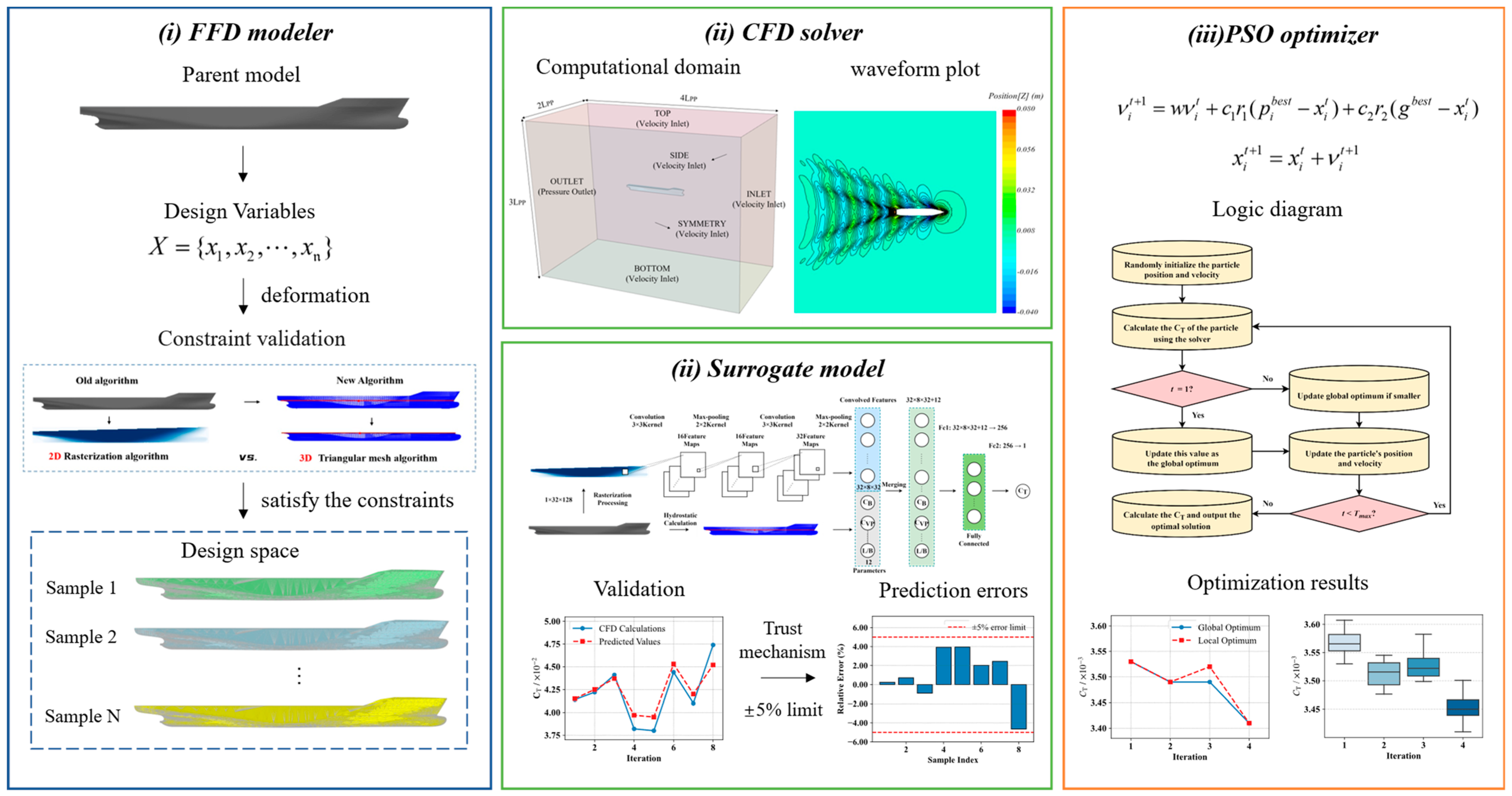
The hull form optimization system developed in this study is built upon the Simulation-Based Design (SBD) framework, integrating key technologies such as optimization algorithms, geometric modeling, and Computational Fluid Dynamics (CFD) into a closed-loop, fully automated optimization process [26], as illustrated in Figure 3. The system is designed to refine hull designs and toward the optimal performance through multiple optimization cycles iteratively, thereby enabling efficient and effective ship design. It consists of three modules: the optimizer, the modeler, and the solver, corresponding, respectively, to optimization techniques, automatic hull geometry modification, and CFD simulation.

The optimizer is responsible for sampling and updating the population using optimization algorithms. These algorithms can be broadly classified into two categories. The first category is gradient-based optimization, which includes methods such as the steepest descent method [27] and Sequential Quadratic Programming (SQP) [28]. The second category is stochastic search optimization, including Particle Swarm Optimization (PSO) [29] and Genetic Algorithms (GA) [30]. In ship design optimization, the optimizer evaluates and refines ship models based on performance-related parameters.

The modeler applies parametric deformation techniques to decode sample data and construct 3D ship models. This process generally falls into two approaches: geometry modification based on ship parameters and geometry modeling–based methods. Parameter-based geometry modification—such as parametric modeling [31] and the Lackenby deformation method [32]—reshapes hull geometry quickly by adjusting parameters like L/B or block coefficient. Geometry modeling–based methods, such as CAD modeling [33] and Free-Form Deformation (FFD) [34], allow not only overall hull deformation but also precise local adjustments, while maintaining control over volume changes before and after deformation.

The solver uses CFD software to perform numerical simulations and hydrodynamic calculations, predicting viscous flow fields around the hull and estimating ship resistance. Based on the Reynolds-Averaged Navier–Stokes (RANS) equations combined with turbulence models, the solver can accurately predict resistance characteristics under free-surface conditions. In other studies, surrogate models such as neural networks [35] and response surfaces [36] have often been used in place of CFD solvers to improve computational efficiency.

These three modules work in close coordination: the optimizer generates design samples, the modeler transforms them into hull geometries, and the solver evaluates their performance. The results are then fed back to the optimizer, guiding the next round of refinement. Through this loop, the design progressively converges toward the optimal hull form.

2.2.1. PSO Optimizer

Ship design and performance optimization problems often feature high-dimensional design spaces and nonlinear constraints. Such complexity limits the effectiveness of purely gradient-based optimization methods in finding global optima [37]. By contrast, swarm intelligence optimization algorithms have become an important tool in engineering optimization, as they do not rely on gradient information, have strong global search capabilities, and are relatively easy to implement [38]. Among these, Particle Swarm Optimization (PSO) has been widely applied to hull form optimization [39] and energy efficiency improvement [40] because of its small number of parameters, fast convergence, and stable performance in various engineering tasks.

Compared with other evolutionary algorithms such as Genetic Algorithms (GA) or NSGA-II, PSO is chosen in this study because it requires fewer control parameters, converges faster in continuous design spaces, and provides reliable performance with relatively low computational overhead. Since the objective of this work is to validate the feasibility of the proposed dual-mode optimization framework rather than to benchmark different optimizers, PSO offers a practical balance between efficiency and robustness under the limited number of expensive CFD-based evaluations [41].

In PSO, each particle represents a candidate solution, and its motion in the search space is determined by both position and velocity. During the iteration process, particles adjust their trajectories based on their own historical best position (personal best, p^best) and the best position found by the swarm (global best, g^best), enabling dynamic evolution of the solutions. The velocity and position are updated using the following equations:

$$v_i^{t+1}=w{v}_i^t+c_1{r}_1(p_i^{best}-x_i^t)+c_2{r}_2(g^{best}-x_i^t)$$

(1)

$$x_i^{t+1}=x_i^t+v_i^{t+1}$$

(2)

Here, $x_i^t$ and $v_i^t$ denote the position and velocity of the particle at iteration, $w$ is the inertia weight, $c_1$ and $c_2$ are learning factors, $r_1,r_2~U(0,1)$ are random numbers that help increase search diversity.

In this study, PSO aims to minimize the total resistance coefficient, with the design variables being the control point parameters of the FFD method. The optimizer first reads the initial positions and velocities of the particle swarm from a historical sample database and evaluates the objective function for each particle. The global best solution is initialized with the state of the first particle, after which the iterative update process begins. In each generation, particle velocities and positions are updated according to Equations (1) and (2), new models are generated, and their performance is evaluated by the solver. The personal and global best values are then updated. When the maximum number of iterations is reached, the current best design is output. The PSO parameter settings used in this study are given in

Table 2. PSO optimizer parameter settings.

$\mathbf{Inertia} \mathbf{Weight} \mathit{w}$	Learning Factor c1	Learning Factor c2	Position Range	Velocity Range
0.3	0.35	0.8	[−1, 1]	[0.04, 0.06]

. The inertia weight (w = 0.3) and learning factors (c₁ = 0.35, c₂ = 0.8) follow recommended values in the literature [42] and have been validated in our previous studies [17]. The relatively small inertia weight promotes local exploitation, while the asymmetric learning factors (c₂ > c₁) prioritize swarm knowledge over individual memory, which accelerates convergence and reduces the number of costly function evaluations. The position range ([−1, 1]) and velocity range ([0.04, 0.06]) are chosen to constrain the FFD control point displacements within realistic bounds: large enough to ensure effective exploration of the design space, but limited to avoid unphysical hull distortions.

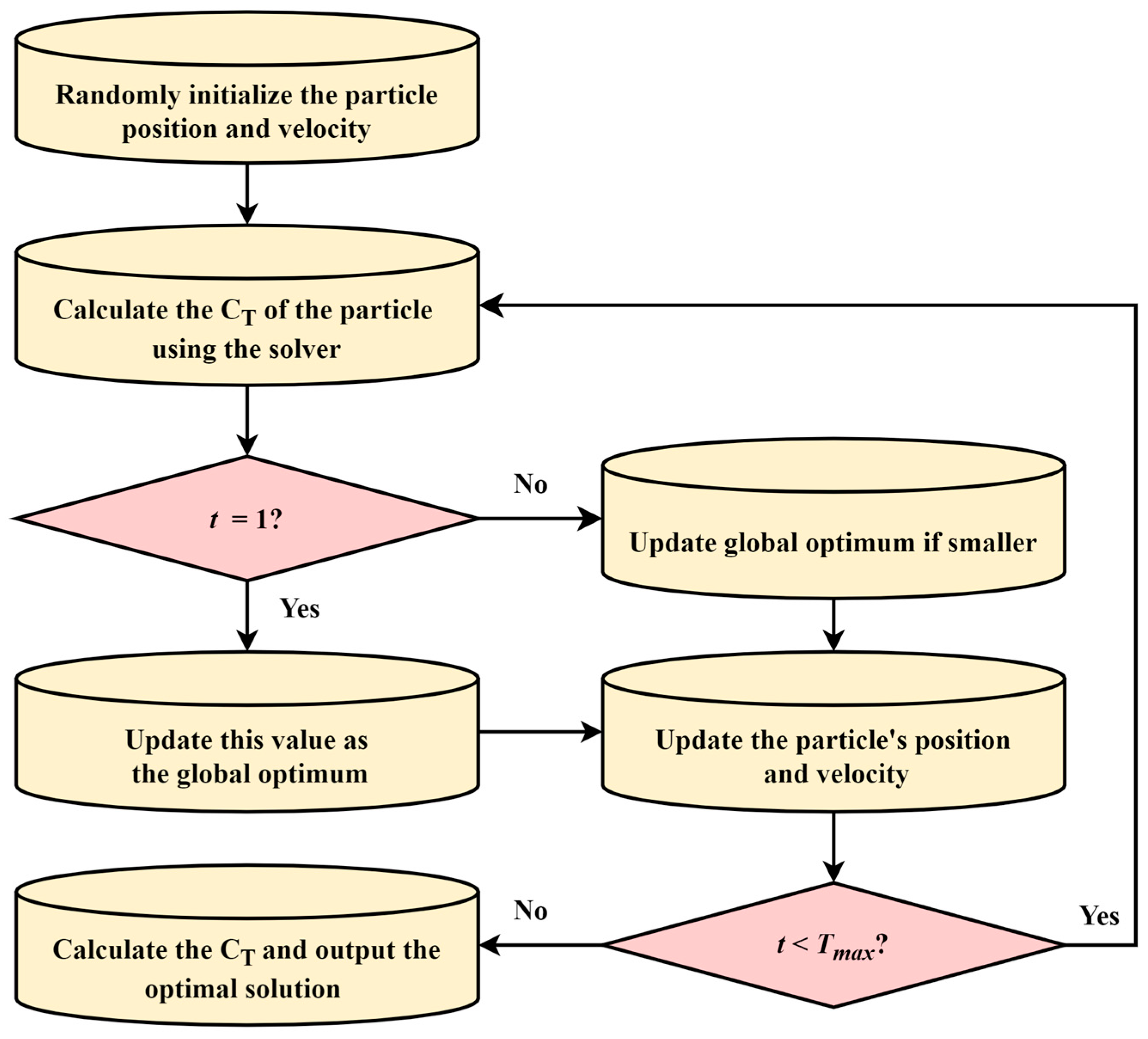
The flow chart of PSO optimizer is illustrated in Figure 4. The initial population is first converted into 3D geometric models by the modeler. The solver then computes the corresponding total resistance coefficient C_T. Based on this performance feedback, the optimizer dynamically adjusts the particle swarm and continues iterating until the termination condition is met. This optimization module, working in conjunction with the modeler and solver, forms the core optimization engine of the SBD framework in this study.

2.2.2. FFD Modeler

In the previous section, the optimizer module has already produced the design variables that describe hull deformations. This section focuses on the selection and implementation of the geometric modeling method, which transforms these abstract parameters into three-dimensional hull geometries for subsequent hydrodynamic performance evaluation. The choice of geometric modeling approach not only affects the expressiveness of the design variables but also directly determines the exploration capability of the design space and the computational accuracy during optimization.

Some popular techniques such as blending methods, Bezier patches, radial basis interpolation, and the Lackenby transformation each have their strengths but also notable limitations. The blending method depends heavily on the initial set of hull forms, making it difficult to go beyond the original geometry. The Bezier patch approach enables precise local shape adjustments but is less efficient for large-scale deformations. Radial basis interpolation offers a small number of design variables and computational flexibility, yet tends to produce distortions when applied to large surface modifications. The Lackenby transformation involves few parameters and is well-suited to global scale changes, but lacks the ability to finely control local surface features [43].

To overcome these drawbacks and enable more flexible, fine-grained, and continuous geometric transformations, this study adopts the Free-Form Deformation (FFD) technique. First proposed by Sederberg and Parry in 1986 [44], FFD has been widely applied in computer graphics, but its systematic application to ship design and optimization has only gained traction in the past decade. The core idea of FFD is to embed the target object in a regular control volume and achieve continuous deformation by moving the positions of control points, thereby allowing both global and local geometry adjustments.

The process begins by establishing a local coordinate system for the control volume enclosing the object. Taking X₀ as the origin and S, T, and U as the three directional vectors, any point X within the control volume can be expressed in the local coordinates as:

$$X_{(s,t,u)}=X_0+sS+tT+uU$$

(3)

Here, s, t, and u are the coordinates of the point in the local system, ranging from [0, 1].

Once the local coordinates are obtained, polynomial basis functions are used to map the control points, as expressed in Equation (4):

$$X_{(s,t,u)}={{\displaystyle \sum }}_{i=0}^l{{\displaystyle \sum }}_{j=0}^m{{\displaystyle \sum }}_{k=0}^n{B}_i^l(s)B_j^m(t)B_k^n(u)\cdot P_{ijk}$$

(4)

where $X_{(s,t,u)}$ represents the position of a parameter point in the deformed space, $P_{ijk}$ is the new position of the $(i,j,k)$ control point, and $B_i^l(s),B_j^m(t),B_k^n(u)$ is the cubic Bernstein basis function.

Figure 5 illustrates the application of Free-Form Deformation (FFD) to hull form modification. The initial hull geometry is embedded within a three-dimensional control lattice composed of uniformly distributed control nodes, with local densification around the fore and aft-body region to enable precise shape adjustments. By displacing selected control points in the x, y, or z directions, the surrounding hull surface deforms smoothly through the FFD interpolation function. These displacement values are later treated as design variables for the optimizer, which employs CFD evaluations to guide the iterative hull optimization process.

The selection of control points in the FFD lattice plays a key role in defining the design space and influencing optimization outcomes. In this study, control points were uniformly distributed overall, with local densification around the fore and aft-body regions. This arrangement provides an appropriate balance between computational efficiency and optimization precision.

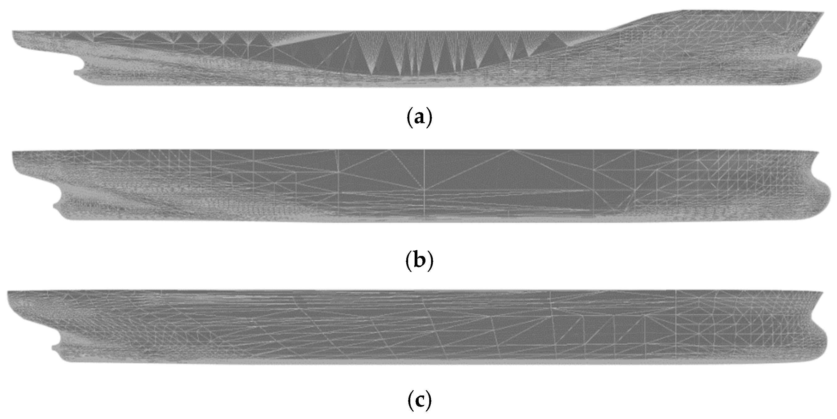
To prevent excessive geometric distortion or displacement-related errors such as variations in displacement volume, the magnitude of control point shifts in the x, y, and z directions is limited to within 2%. Additionally, a geometry verification algorithm is implemented to ensure modeling accuracy. To provide a clearer explanation for Figure 6, the verification algorithm works on the deformed STL geometry through a multi-step process: (a) The algorithm first parses the STL file to extract the vertices and normal vectors of all triangular facets. (b) The waterplane contour at a specified draft is precisely determined by calculating the intersection lines between the triangulated surface and the draft plane. (c) These intersection points are sorted and connected to form a closed, non-intersecting polygon representing the waterline. (d) The closed waterplane polygon is then triangulated into a set of simple triangles for which area and centroid calculations are straightforward. (e) Finally, the hydrostatics are computed by integrating the properties of these triangles, ensuring high numerical precision necessary for reliable CFD evaluation.

As illustrated in Figure 7, compared with the 2D rasterization algorithm mapping the 3D surface offset on the central plane and calculating hydrostatics based on projected area, the proposed 3D triangular mesh algorithm, however, preserves the 3D features of the original geometry. As a result, it achieves significantly higher accuracy for parameters closely related to 3D volume and surface area, such as wetted surface area (m²) and displacement volume (m³).

To evaluate the accuracy of the algorithms, the KCS benchmark model is used. The reference values (“Reference Data”) for all hull form parameters are obtained from the complete geometry database provided by the official SIMMAN 2008 website, which serves as the benchmark for this study. The evaluation results of both the conventional and proposed algorithms are summarized in

Table 3. Evaluation results of conventional and proposed algorithms for hull form parameter calculation in the KCS benchmark case.

Parameter	Symbol/Unit	Reference Data 1	Old	Error 1 2	New	Error 2 2
Displacement	$\nabla$/m3	1.646	1.557	5.4%	1.647	0.06%
Square coefficient	CB	0.642	0.613	4.52%	0.642	0.00%
Prismatic coefficient	CP	0.654	0.656	0.30%	0.656	0.30%
Waterline coefficient	CWP	0.822	0.791	3.77%	0.821	0.12%
Medium cross-section Coefficient	CM	0.985	0.955	3.05%	0.978	0.71%
Wetted surface area	Sw/m2	9.554	8.878	7.08%	9.543	0.12%

¹ Reference Data of KCS is provided by the official website of SIMMAN 2008 [24]. ² Error 1 and Error 2 denote the relative deviations of the Conventional and Proposed algorithms from the reference data, respectively.

. The proposed method limits calculation errors against the reference data for all hull form parameters to within 1% (maximum is 0.71% from C_M), with a particularly notable improvement in displacement volume accuracy.

2.2.3. Dual-Mode Solver

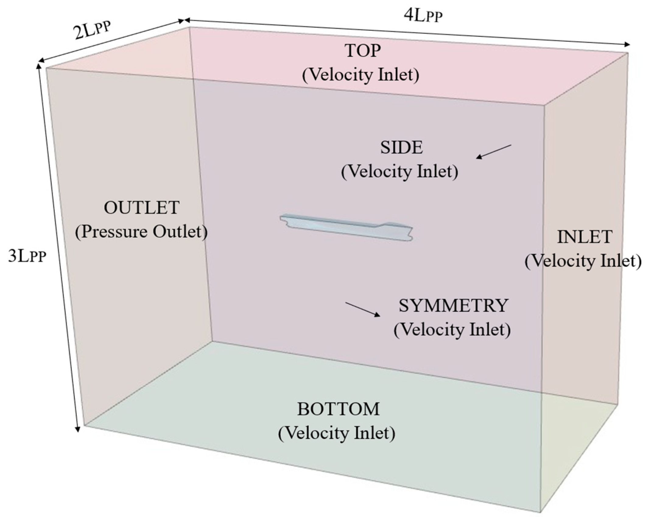
In the previous section, the FFD modeler converted the design variables output by the optimizer into computable three-dimensional hull models. To assess the hydrodynamic performance of these designs, a numerical solver is required to simulate the surrounding flow field and predict resistance. The CFD solver is the core tool for this task. Its fundamental principle involves discretizing the governing equations of fluid motion, then solving them iteratively on a computational grid to obtain the velocity field, pressure field, and total resistance around the hull. Widely used in ship design, CFD offers high-accuracy numerical predictions that complement physical experiments, providing a robust physical basis for performance optimization.

However, high-fidelity CFD simulations come at a steep computational cost, particularly in hull form optimization, where numerous candidate designs must be evaluated repeatedly. For example, resistance prediction for a single hull at full scale with a refined mesh can require several hours or more, making large-scale exploration of the design space impractical.

To address this challenge, surrogate models have been increasingly introduced into hydrodynamic performance prediction in recent years. The core idea is to employ data-driven methods to learn the nonlinear mapping between input features and target performance, thereby reducing computational demands while sacrificing only minimal accuracy [45]. Among these, deep learning approaches, owing to their powerful feature extraction and generalization capabilities, have shown strong performance in tasks such as hull resistance prediction [46] and ship speed estimation [47]. In particular, Convolutional Neural Networks (CNNs), which excel at capturing both local and global geometric features, have proven well-suited for hydrodynamic performance prediction [48].

Building on this foundation, the present study proposes a hydrodynamic performance evaluation framework that integrates a two-dimensional Convolutional Neural Network (2D CNN) with a dual-mode mechanism. The method dynamically switches between CFD simulation and surrogate model prediction during optimization, striking a balance between computational accuracy and efficiency to enable fast yet reliable hull performance assessment.

Here, the 2D CNN serves as the surrogate model, and its logical structure is illustrated in Figure 8. The 2D CNN effectively captures local spatial features on the hull surface and extracts multi-scale geometric patterns through convolution operations, enhancing both generalization capability and prediction accuracy.

In the data preprocessing stage, the hull surface is projected onto a two-dimensional grid and rasterized at a fixed resolution of 32 × 128, yielding a 2D tensor. The network input consists of two parts: (1) The rasterized 2D hull geometry data. (2) A 12 × 1 vector containing principal dimensions and form coefficients.

The raster data are first processed through the convolutional network to extract features, after which the 12 × 1 parameter vector is concatenated with the flattened convolutional features.

The 2D CNN architecture designed in this study comprises two convolutional layers and two pooling layers. The convolution operations capture multi-scale local geometric features of the hull surface, while pooling operations reduce data dimensionality. Finally, the flattened convolutional features are fused with the 12-dimensional parameters and passed through fully connected layers to perform regression, producing the total resistance coefficient C_T as the output.

The model is trained using a dataset of 200 pre-computed CFD samples, split into 80% for training and 20% for validation.

Table 4. Key hyperparameters and training configuration of the CNN model.

Item	Data Split	Loss Function	Optimizer	Batch Size	Epochs	Learning Rate	Activation
Setting	80% training, 20% test	MSE	Adam	10	50	0.001	LeakyReLU

summarizes the key hyperparameters and training configuration.

The prediction accuracy of the CNN model is evaluated on the test set. As shown in Figure 9, the scatter plot of predicted versus true C_T values indicates that most points cluster near the ideal 1:1 line, indicating high predictive accuracy.

In this study, the input dataset is inherently high-dimensional, consisting of 12 principal coefficients together with 4096 rasterized geometric features. Traditional methods such as Kriging and RSM typically struggle to maintain predictive accuracy when applied to such high-dimensional and highly nonlinear data, as their scalability and feature extraction capability are limited. By contrast, CNNs are well-suited to this task because convolutional layers can effectively capture local and global geometric patterns while mitigating the curse of dimensionality.

For a horizontal comparison, reference values for the Kriging model and RSM are taken from relevant studies and are listed together with the CNN results in

Table 5. Comparison of CNN, RSM, and Kriging models on the test set.

Model	Metric	NRMSE	R2	eavg
CNN	CT	0.042	0.979	0.003
RSM [49]	RT	0.070	0.939	0.049
Kriging [50]	RT	0.015	0.955	0.009

. As can be seen, the proposed CNN achieves a normalized root mean square error (NRMSE) of 0.042 and an R² of 0.979, outperforming the RSM (NRMSE = 0.070, R² = 0.939) and Kriging (NRMSE = 0.015, R² = 0.955) baselines. These results demonstrate that the CNN model provides more accurate resistance prediction in the context of high-dimensional hull-form data.

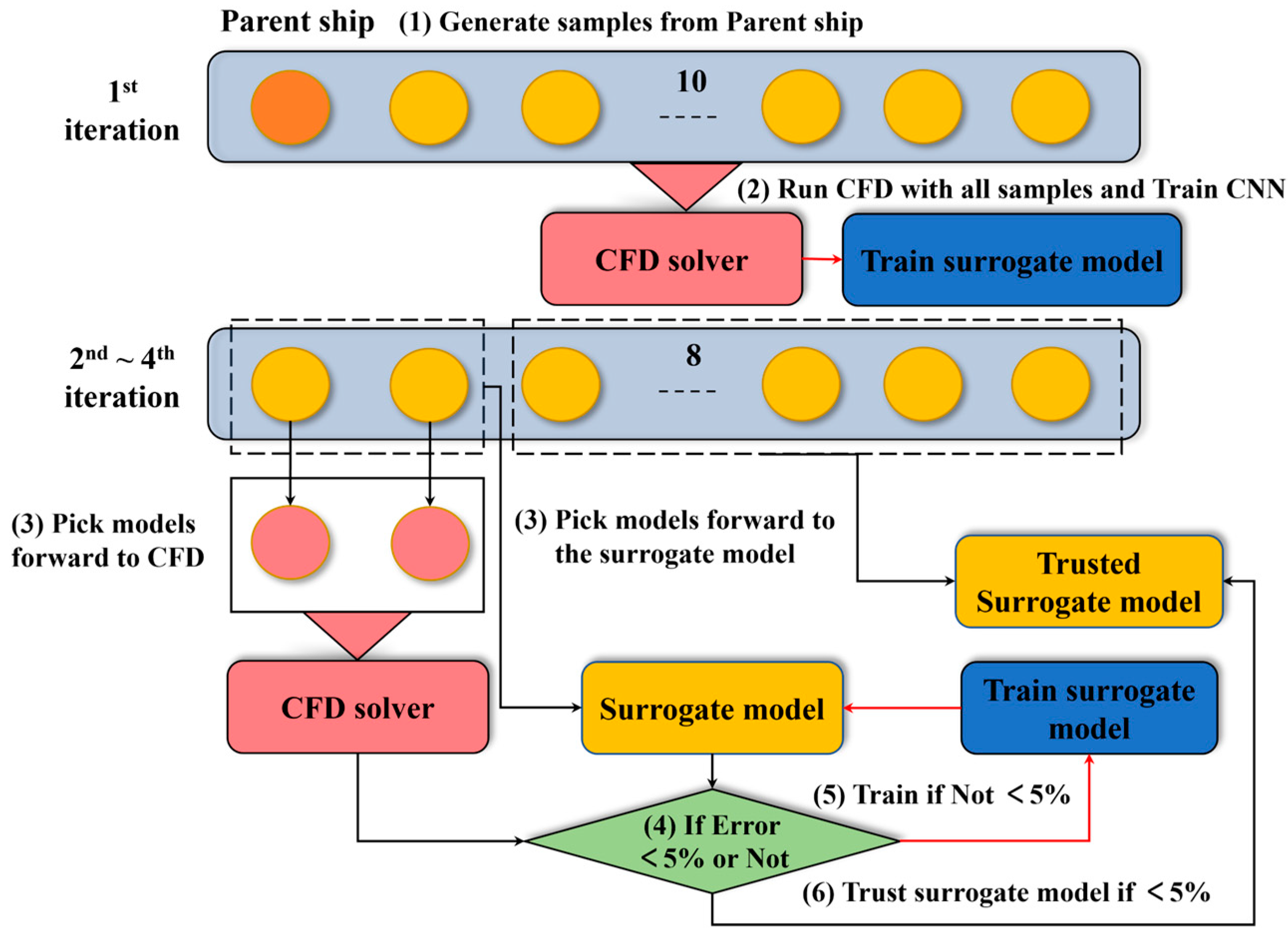
The overall workflow is illustrated in Figure 10 and can be divided into three main stages:

1.

Initial Exploration Stage: At the start of optimization, the CFD solver is applied to all three-dimensional hull samples. The resulting high-fidelity hydrodynamic data are used to train the surrogate model, providing both an accurate performance baseline and guidance for determining promising search directions;

2.

Hybrid-Mode Iteration Stage: From the second optimization cycle onward, a hybrid strategy is applied: Only a subset of ship designs is evaluated using CFD, while the surrogate model predicts the remaining designs. The choice of evaluation method depends on the prediction error of the surrogate model:

• Case 1: If the surrogate model’s prediction error is below 5%, the model’s output is accepted directly, improving computational efficiency;
• Case 2: If the surrogate model’s prediction error exceeds 5%, CFD is used for that sample. The new CFD data are then incorporated into retraining the surrogate model until its error falls below the 5% threshold.

3.

Final stage: Once the maximum number of optimization cycles is reached, the final optimized hull form and its performance metrics are output.

Table 6. Demonstrative short-term test conditions.

Ship	Cycles	Population Size	CFD Samples	Time Step (s)	Simulation Time (s)	Speed (m/s)
JBC	3	8	4	0.03	0.3	1.179

presents a short-term demonstrative case designed to validate the functionality of the dual-mode solver and to illustrate its working principle in a computationally affordable manner. The simulation duration is limited to 0.3 s, and the number of cycles and samples per cycle are intentionally kept small, allowing a clear demonstration of the stochastic sampling, optimization, and CFD verification procedure, while avoiding excessive computational overhead. The chosen ship speed corresponds to the standard JBC test condition from the Tokyo 2015 CFD Workshop, ensuring representativeness of the setup.

The dual-mode solver’s behavior in this test is shown in Figure 11:

• Figure 11a: First iteration—all samples are evaluated using both CFD and the 2D CNN surrogate model for comparison. Blue solid lines indicate CFD results, and red dashed lines indicate surrogate predictions.
• Figure 11b: Second iteration—CFD is applied only to the first 4 samples, with the rest predicted by the surrogate model.
• Figure 11c: Third iteration—followed the same computation mode as the second iteration.

The relative error between surrogate predictions and CFD calculations is computed according to Equation (5). If the error for a given cycle is within 5%, the surrogate model is considered reliable and is used for the remaining samples; otherwise, additional CFD calculations are performed to retrain the model until the error falls below the threshold.

$$ϵ={\displaystyle \frac{C_{T,\mathrm{Predict}}-C_{T,\mathrm{CFD}}}{C_{T,\mathrm{CFD}}}}\times 100\%$$

(5)

The choice of a 5% error threshold for surrogate model acceptance is supported by empirical studies in naval architecture, such as Chen et al. [51], who reported surrogate model errors in the range of 3–7% for similar ship resistance prediction tasks. The error evaluation results for the short-term test are presented in Figure 12. Across all iterations, the surrogate model’s prediction error remained below 5%, confirming its reliability and applicability in the hybrid computation framework.

2.3. CFD Simulation

Before carrying out the optimization task, it is first necessary to perform hydrodynamic calculations on the parent ship as the starting point of the optimization. During the numerical calculation process, in order to reduce the calculation cost, this study scaled down the three ship types KCS, KVLCC1 and JBC, and only selected the scaled half-ship for numerical simulation. The calculation domain adopts a rectangular calculation domain, and its dimensions are set to 4L_PP, 2L_PP and 3L_PP, respectively, and the coordinate origin is located at the intersection of the hull station 0 and the still water surface. In terms of boundary condition setting, the outlet is set as the pressure outlet, the center plane and the symmetry plane are symmetry boundaries, and the remaining boundaries are set as velocity inlets. In addition, in order to reduce the influence of wave reflection on the calculation results, wave-damping boundary conditions are applied at the inlet, outlet and side. The calculation domain setting and boundary conditions are shown in Figure 13.

To ensure numerical reliability, a quantitative grid convergence study is carried out following the ITTC recommended procedure. As shown in Table 7, three systematically refined mesh sets are generated using a constant mesh refinement ratio of $r_G=\sqrt{2}$, with baseline mesh sizes of 0.1 m, 0.1414 m, and 0.2 m, yielding three mesh sets: $S_{G1}$, $S_{G2}$, $S_{G3}$.

$$R_G={\displaystyle \frac{S_{G2}-S_{G1}}{S_{G3}-S_{G2}}}$$

(6)

where $S_{G1}$, $S_{G2}$ and $S_{G3}$ denote the computed results for the fine, medium, and coarse meshes, respectively.

The uncertainty calculation results are shown in Table 8, the calculated R_G values for the KCS, KVLCC1, and JBC hulls are 0.136, 0.515, and 0.737, all within the range (0, 1). This confirms that the resistance results satisfy the ITTC convergence criterion and demonstrate grid convergence [52]. The U_G values are below 2.2% in all cases, indicating that the mesh resolution is sufficient for reliable resistance prediction. Balancing computational cost and accuracy, the medium mesh $S_{G2}$ is selected for all subsequent simulations.

Table 7. Numerical resistance results for different mesh densities compared with experimental data.

Hull Form	KCS				KVLCC1				JBC
–	$S_{G3}$	$S_{G2}$	$S_{G1}$	D  1	$S_{G3}$	$S_{G2}$	$S_{G1}$	D  1	$S_{G3}$	$S_{G2}$	$S_{G1}$	D  1
Grid cells (×104)	86.24	150.86	283.29	–	50.48	111.68	212.24	–	99.15	179.85	262.5	–
RT (N)	81.10	80.66	80.60	80.13	13.02	13.35	13.52	13.87	34.48	34.86	35.14	36.37

¹ D denotes the experimental measurement of total resistance [53,54,55].

Table 7. Numerical resistance results for different mesh densities compared with experimental data.

Hull Form	KCS				KVLCC1				JBC
–	$S_{G3}$	$S_{G2}$	$S_{G1}$	D  1	$S_{G3}$	$S_{G2}$	$S_{G1}$	D  1	$S_{G3}$	$S_{G2}$	$S_{G1}$	D  1
Grid cells (×104)	86.24	150.86	283.29	–	50.48	111.68	212.24	–	99.15	179.85	262.5	–
RT (N)	81.10	80.66	80.60	80.13	13.02	13.35	13.52	13.87	34.48	34.86	35.14	36.37

¹ D denotes the experimental measurement of total resistance [53,54,55].

Table 8. Mesh uncertainty analysis.

RT	RG	PG	δRE*G	CG	UG/%
KCS	0.136	5.749	0.00947	6.333	0.138
KVLCC1	0.515	1.914	−0.181	0.941	1.302
JBC	0.737	0.881	−0.784	0.357	2.156

Table 8. Mesh uncertainty analysis.

RT	RG	PG	δRE*G	CG	UG/%
KCS	0.136	5.749	0.00947	6.333	0.138
KVLCC1	0.515	1.914	−0.181	0.941	1.302
JBC	0.737	0.881	−0.784	0.357	2.156

2.4. Two Optimization Schemes

In the field of hull form optimization, traditional approaches generally fall into two categories: full CFD-based optimization and full surrogate model-based optimization.

The full CFD approach, such as that implemented in the CAESES optimization platform, relies entirely on CFD solvers to perform high-fidelity simulations for every hull generated in each optimization iteration. This method provides precise flow field data and accurate resistance predictions. However, it is computationally expensive and demands substantial computing resources, often requiring several days or even weeks to complete a single optimization process.

By contrast, surrogate model-based optimization replaces the CFD solver with a pre-trained data-driven model to deliver rapid performance predictions. While this approach dramatically increases computational efficiency, it inevitably sacrifices some degree of accuracy.

To address this trade-off, the present study employs a dual-mode solver that combines the strengths of both methods. This hybrid approach leverages CFD for accuracy and a convolutional neural network surrogate model for efficiency, aiming to minimize accuracy loss while markedly reducing computational time.

The present work focuses on resistance optimization as the first step, since total resistance in calm water remains the most fundamental and widely adopted performance metric for hull form evaluation. Compared with propulsion and seakeeping, resistance can be directly obtained from high-fidelity CFD simulations with relatively low uncertainty, which makes it particularly suitable for verifying the feasibility of the proposed dual-mode optimization strategy. By contrast, seakeeping and propulsion performance involve additional complexities, which substantially increase the computational cost and introduce uncertainties beyond the scope of this initial study. For these reasons, the present work limits the scope to resistance, while the extension of the hybrid optimization framework to seakeeping and propulsion will be considered in future research.

The proposed hybrid optimization strategy is applied to three benchmark hulls, KCS, KVLCC1, and JBC, each at its respective design speed, to minimize total resistance. For KCS, the objective function is given in Equation (7), while for KVLCC1 and JBC it is given in Equation (8) [56]:

$$Min f=R_T (Fr=0.26)$$

(7)

$$Min f=R_T (Fr=0.142)$$

(8)

Here, $R_T$ denotes the total resistance in still water.

To ensure that the hydrodynamic characteristics remain consistent before and after optimization, the change in displacement is constrained to within 1%. The displacement constraint is expressed as:

$${\displaystyle \frac{\left|\nabla -{\nabla }_{original}\right|}{\nabla }}\le 1\%$$

(9)

where $\nabla$ represents the displacement.

To validate the effectiveness of the proposed method, we use full CFD optimization in CAESES as a baseline, keeping all experimental conditions identical, including hardware configuration, baseline hull models, and initial simulation cases. The experiments are run on the laboratory’s high-performance computing server equipped with dual Intel Xeon Gold 6326 CPUs (2.90 GHz, 32 cores in total).

For reference, under the JBC test condition with an 18 s simulation window, a single sample requires approximately 34.5 min of computation. Considering computational cost and resource usage, the optimization settings for the three hull forms are summarized in

Table 9. Optimization settings for the three hull forms.

Hull Form	Time Step (s)	Simulation Time (s)	Speed (m/s)	Iterations
KCS	0.03	40	2.196	40
KVLCC1	0.03	18	0.994	40
JBC	0.03	18	1.179	40

. The optimization settings are determined based on numerical stability and convergence requirements. Specifically, the time step (0.03 s) represents a balance between stability and computational cost, which is widely adopted in CFD-based ship resistance simulations. The simulation time for each hull form is established according to the resistance convergence behavior: KVLCC1 and JBC reach a stable signal within 18 s, while KCS requires longer time. The ship speeds correspond to the design speeds of the three hull forms, ensuring realistic and practically meaningful optimization conditions. The number of iterations is set to 40 as a compromise between optimization accuracy and computational efficiency, following preliminary calibration tests.

2.4.1. CAESES Optimization Scheme

The CAESES-based optimization adopts a serial, single-sample evolutionary strategy, with a population size of 1 and 40 consecutive iterations. The design variables include three global parameters and one bow-specific parameter: ΔC_P and ΔX_CB are allowed to vary by ±1%. The design waterline entrance width (Y) and bow bulb angle (Z) are expressed in dimensionless relative values, with the ranges summarized in

Table 10. Design Variables and Variation Ranges for Hull Optimization.

Variable Description	Symbol	Variation Range			Geometry Reconstruction Method
		KCS	KVLCC1	JBC
Prismatic coefficient variation	ΔCP	[−0.01, 0.01]	[−0.01, 0.01]	[−0.01, 0.01]	Lackenby
Longitudinal position of the center of buoyancy	ΔXCB	[−0.01, 0.01]	[−0.01, 0.01]	[−0.01, 0.01]	Lackenby
Inflow-end width of design waterline	Y	[−0.1, 0.1]	[−0.02, 0.02]	[−0.02, 0.02]	Brep Morphing
Bulbous bow angle	Z	[−0.1, 0.1]	[−0.1, 0.1]	[−0.2, 0.2]	Delta Shift

. The variation ranges of the design variables are selected according to established practices in ship hydrodynamic optimization, supported by literature guidelines and preliminary validation. The prismatic coefficient (ΔC_P) and the longitudinal position of the center of buoyancy (ΔX_CB) are allowed to vary within ±1%, which is a conventional range in the application of the Lackenby transformation, ensuring realistic geometry without excessive deformation. The range of the design waterline entrance width (Y) depends on the sensitivity of each hull: a wider interval is used for KCS, while narrower bounds are adopted for KVLCC1 and JBC to prevent non-physical shapes. Similarly, the bulbous bow angle (Z) is adjusted within ranges reflecting hull-specific bow geometry.

To maintain diversity in the design space, three geometric reconstruction methods, Lackenby, Brep Morphing, and Delta Shift are used to target multi-scale hull modifications: overall translation, entrance width adjustment, and bulbous bow angle variation, respectively. Figure 14 highlights the corresponding hull regions affected by each method.

The optimization process (Figure 15) begins with Sobol sequence sampling for an initial, space-filling exploration of the design space. From these samples, a subset of promising hull forms is identified. The Tsearch optimization algorithm is then applied in the vicinity of the best-performing samples to converge on the final optimized hull form.

2.4.2. Optimization Scheme Using the Proposed System

The proposed system employs a parallel evaluation strategy, with a population size of 10 over 4 optimization rounds. The total number of evaluated samples matches that of the CAESES scheme for fair comparison.

The deformation region is identical to that shown in Figure 16, and the optimization variables are defined as follows:

• Figure 16a: y—bulbous bow width; z—upward curvature of the bulbous bow;
• Figure 16b: y—bow control point width;
• Figure 16c: y—stern control point width.

To avoid geometric distortion and ensure the numerical stability of hydrodynamic simulations, the variation range of each optimization variable is restricted to within ±2% of its original coordinate value.

As shown in

Table 11. SBD system cases.

Hull Form	Iterations	Population Size	CFD Validations per Iteration
KCS	4	10	2
KVLCC1	4	10	2
JBC	4	10	2

and Figure 17, each iteration generates 10 hull samples. In the first iteration, all samples are evaluated using the STAR-CCM+ CFD solver, and the corresponding results are used to train the CNN surrogate model. From the second iteration onwards, the framework switches to a hybrid strategy: among the newly generated samples, only two are selected for both CFD solution and surrogate model calculations to verify the surrogate model’s accuracy. An error-checking mechanism is also added: if the surrogate model’s prediction error remains below 5%, the surrogate model is trusted, and the remaining samples are evaluated using the trusted surrogate model; otherwise, the solution is solved using CFD calculations, and the model is retrained and calibrated. This setup maintains prediction accuracy while substantially reducing computational cost by reducing the number of CFD simulations.

3. Results

3.1. Comparison of Optimization Processes

This section compares the optimization process and performance outcomes between the CAESES platform and the proposed SBD system across three hull forms. In the CAESES scheme, each CFD simulation is executed with 60 processes dedicated to a single case, so that only one design is evaluated at a time. In contrast, the proposed SBD system adopts a particle swarm optimization (PSO) algorithm with a population size of 10 per generation. Here it should be noted that population size does not equate to the number of parallel CFD cases. Instead, in our implementation the 60 CPU processes are distributed across 5 concurrent CFD simulations (12 processes per case), enabling multiple candidate designs to be evaluated simultaneously. This parallel evaluation strategy significantly reduces the wall-clock time per generation, while maintaining the same total number of evaluations as in the baseline.

The efficiency gain comes from a more balanced use of computing resources. When all CPU processes are assigned to a single CFD case, adding more processes does not always make the simulation much faster because of increasing communication overhead. In contrast, running several CFD cases at the same time with fewer processes per case makes better use of the available CPUs. This approach improves hardware utilization.

The CAESES optimization results are shown in Figure 18, where the Sobol and Tsearch algorithms each perform 20 iterations, with the results of a single sample displayed per iteration. The optimization behavior differs among the hull forms:

• KCS (Figure 18a): Considerable fluctuations in total resistance coefficient during initial iterations reflect broad design space exploration by the Sobol algorithm;
• KVLCC1 (Figure 18b): Large-amplitude oscillations of the resistance coefficient through the early-mid stages indicate extensive global search with limited convergence. Subsequent application of Tsearch algorithm achieves notable resistance reduction;
• JBC (Figure 18c): Despite persistent volatility in resistance coefficient, the combined method demonstrates clear convergence in final iterations, yielding lower resistance than standalone Sobol optimization.

In contrast, the iteration process of the proposed SBD system is illustrated in Figure 19 and Figure 20. Due to the parallel evaluation strategy, four rounds of iterations are plotted. In Figure 19, red and blue lines denote the global optimum and the best solution per iteration, while the box plots in Figure 20 depict solution distributions, aiding in the assessment of dispersion and stability.

• KCS (Figure 19a and Figure 20a): Convergence curves show a rapid initial decrease in resistance coefficient (C_T), reaching a near-optimal region by iteration 4 and stabilizing. Corresponding box plots exhibit a continuous and marked narrowing of the solution range, indicating low dispersion and a highly concentrated, stable solution set;
• KVLCC1 (Figure 19b and Figure 20b): Convergence curves display an overall decreasing trend but with pronounced fluctuations, suggesting high sensitivity of C_T to changes in design variables. Box plots maintain consistently wide ranges, exhibit large boundary variations, and contain outliers, indicating high dispersion and relatively unstable optimization behavior;
• JBC (Figure 19c and Figure 20c): Convergence curves exhibit transient increases before converging to the near-optimal region, demonstrating the algorithm’s ability to escape local optima. Box plots show a marked narrowing of the solution range in later iterations, signifying reduced dispersion and stabilization during the final convergence phase.

Table 12. Comparison of optimization time between the SBD system and the conventional full-CFD approach.

Hull Form	SBD System Opt. Time	CAESES Opt. Time	Efficiency Gain (%)
KCS	24 h 29 min	54 h 53 min	44.61%
KVLCC1	12 h 34 min	26 h 05 min	48.18%
JBC	12 h 26 min	25 h 18 min	49.14%

compares the optimization time between the proposed SBD system and the conventional full-CFD approach in CAESES. The SBD system, which incorporates a dual-mode solver, completes the optimization process in significantly less time across all three hull forms: KCS, KVLCC1, and JBC. Specifically, the SBD system reduces the optimization time by 44.61% for KCS, 48.18% for KVLCC1, and 49.14% for JBC.

This notable improvement in efficiency, nearly halving the time required for KVLCC1 and JBC, is primarily due to a reduction of 24 full CFD evaluations achieved through the strategic use of the dual-mode solver. By combining high-fidelity CFD simulations with faster surrogate evaluations, the SBD system minimizes computational expense while maintaining optimization quality, substantially accelerating the overall workflow.

3.2. Comparison of Hydrodynamic Performance

To systematically evaluate the effects of the two ship optimization schemes, this section compares the wave pattern characteristics and resistance performance improvements based on the experimental data from both the CAESES system and the proposed system.

First, in terms of wave pattern comparison, Figure 21 presents the free surface wave cut results at a transverse section located 0.1 times the L_PP from the centerline for the three ships, optimized by the proposed system and the CAESES, respectively:

• KCS (Figure 21a): The parent hull exhibits relatively large wave amplitudes near the sides. Both the CAESES hull and the SBD hull show reduced wave amplitudes along the sides compared to the parent hull. Furthermore, at the stern, the wave crest of the SBD hull is lower than that of the parent hull and the CAESES hull;
• KVLCC1 (Figure 21b): Both optimization methods substantially reduce stern wave height. The wave pattern becomes almost flat, showing that the waves are being well controlled. The wave amplitude along the sides is also smaller than that of the parent hull;
• JBC (Figure 21c): The parent and optimized hulls show minor variations along the bow and sides. For both optimization methods, the wave crests at the bow are slightly lower and the wave troughs slightly deeper compared to those of the parent hull, while along the sides, the wave crests are slightly higher. The wave profiles in other regions remain largely consistent.

To complement these qualitative observations,

Table 13. Quantitative comparison of bow and stern wave height reductions for representative hulls.

Ship	Region	Parent (m)	CAESES (m)	Reduction 1	SBD (m)	Reduction 2
KCS	Bow crest	0.0223	0.0220	1.34%	0.0214	4.04%
	Bow trough	−0.0365	−0.0273	25.21%	−0.0348	4.66%
	Stern crest	0.0289	0.0308	−6.57%	0.0252	12.80%
	Stern trough	−0.0257	−0.0240	6.61%	−0.0234	8.95%
KVLCC1	Bow crest	0.0108	0.0106	1.85%	0.0105	2.78%
	Bow trough	−0.0159	−0.0155	2.52%	−0.0166	−4.40%
	Stern crest	0.0136	0.0089	34.56%	0.0096	29.41%
	Stern trough	−0.0124	−0.0093	25.00%	−0.0099	20.16%
JBC	Bow crest	0.0137	0.0130	5.11%	0.0121	11.68%
	Bow trough	−0.0218	−0.0219	−0.46%	−0.0208	4.59%
	Stern crest	0.0094	0.0094	0%	0.0099	−5.32%
	Stern trough	−0.0109	−0.0109	0%	−0.0109	0%

Reduction 1 and Reduction 2 denote the percentage deviations of the CAESES and SBD results from the parent data, respectively.

summarizes the quantitative wave height reductions at bow and stern crests and troughs for representative hulls. For the KCS hull, the proposed SBD system achieved a notable reduction in stern crest height (12.80%) and outperformed the CAESES baseline in side wave reduction, though CAESES slightly outperformed SBD at the stern crest. For the KVLCC1 hull, both methods effectively reduced stern wave heights by roughly 29–35%, confirming the visual impression of a flattened stern wave pattern. For the JBC hull, improvements were relatively modest, with the proposed system achieving an 11.68% reduction in bow crest height.

In addition to wave characteristics, the total resistance coefficient is a key metric for evaluating optimization performance.

Table 14. Optimization effect of the total resistance coefficient.

Hull	CT (×10−3) Before Opt.	CT (×10−3) After Opt.		CT Reduction (%)
		SBD System	CAESES	SBD System	CAESES
KCS	3.53	3.41	3.44	3.40%	2.55%
KVLCC1	4.05	3.89	3.89	3.95%	3.95%
JBC	4.02	3.91	3.93	2.74%	2.23%

summarizes the total resistance coefficients for the three hull forms before and after optimization using the SBD system and the conventional full-CFD approach in CAESES. Both optimization approaches effectively reduce the total resistance coefficient. For the KCS and JBC, the performance of the SBD system is generally comparable to that of CAESES, with minor improvements observed in some cases; for the KVLCC1, both methods yield essentially equivalent results.

It should be noted that reduction efficiency is influenced by factors such as design variable ranges, initial hull conditions, and simulation settings, and thus some variability in results is expected. Importantly, the proposed SBD system, by integrating CFD simulations with a surrogate model in a dual-mode solver, substantially improves computational efficiency while maintaining effective resistance reduction.

3.3. Comparison of Hull Form Optimization

This subsection presents the results of hull optimization using the two approaches, highlighting the hulls with minimum total resistance relative to the original designs.

Table 15. Hull form coefficients before and after optimization.

Hull Form	Model	L/B	B/T	L/T	CB	CVP	CWL	$\nabla$ (m3)
KCS	Parent ship	7.56	2.98	22.56	0.642	0.782	0.821	1.65
	Optimized ship	7.56	2.98	22.56	0.643	0.781	0.823	1.65
KVLCC1	Parent ship	5.75	2.79	16.04	0.797	0.893	0.893	1.17
	Optimized ship	5.75	2.79	16.04	0.791	0.889	0.890	1.16
JBC	Parent ship	6.47	2.73	17.63	0.844	0.929	0.910	2.79
	Optimized ship	6.47	2.73	17.63	0.839	0.930	0.902	2.77

summarizes the main hull form coefficients before and after optimization for the three hulls. It can be observed that the principal dimensions remain largely unchanged, and the displacement variation is within 1%, satisfying the design constraints.

The hull lines before and after optimization are compared in Figure 22 and Figure 23, where the blue lines represent the original hull forms and the red lines indicate the optimized shapes. Key observations for each hull are as follows:

• KCS (Figure 22a and Figure 23a): Post-optimization contraction of forebody sectional area with improved hull transition continuity. Stern reshaping achieves slenderized form and increased waterline flare angle;
• KVLCC1 (Figure 22b and Figure 23b): Negligible forebody modifications observed. Stern exhibits thinner near the transom region than others;
• JBC (Figure 22c and Figure 23c): Inward contraction of waterline forebody profile accompanied by enhanced stern curvature uniformity.

3.4. Validation of Optimization Results

To further evaluate the hydrodynamic performance of the optimized hulls, this section conducts a validation study based on pressure distribution and resistance–speed relationships, ensuring the effectiveness and reliability of the optimization.

The pressure coefficient C_P is a nondimensional parameter commonly used to characterize pressure distribution on a body surface. It is defined as [57]:

$$C_p={\displaystyle \frac{P-P_0}{0.5\rho U_0^2}}$$

(10)

where P is the local static pressure, P₀ is the reference pressure, $\rho$ is the fluid density, and U₀ is the inflow velocity. A positive C_P indicates a region of higher-than-reference pressure, while a negative C_P corresponds to a low-pressure zone. This makes C_P particularly useful for visualizing flow features.

In terms of pressure distribution, Figure 24 presents the comparison of pressure coefficients around the bow region before and after optimization:

• KCS (Figure 24a): Post-optimization, the bulbous bow exhibits a noticeable downward shift, as evidenced by the high-pressure region (C_P 0.44 to 1.00) extending slightly lower along the bow. The transition between these high-pressure zones appears more gradual and uniform, with contour lines becoming less dense compared to the pre-optimization state, suggesting a reduction in abrupt pressure gradients;
• KVLCC1 (Figure 24b): After optimization, the pressure concentration at the center of the bulbous bow is alleviated, with the peak pressure (C_P around 1.00) showing a broader and less intense red zone compared to the pre-optimized state. The slight upward tilt of the bulbous bow is indicated by the upward shift in the high-pressure contour lines, resulting in a reduced bow wave amplitude. The pressure recovery zone transitions more steeply, with tighter contour spacing in the mid-pressure range (C_P 0.10 to 0.40), enhancing airflow attachment;
• JBC (Figure 24c): The optimized design shows a reduced high-pressure area at the forward bow (C_P 0.64 to 1.00), where the red and yellow zones are smaller and less expansive compared to the pre-optimization state, indicating a decrease in peak pressure intensity. Simultaneously, the low-pressure region beneath the hull (C_P −0.80) has contracted, with the blue contour lines receding toward the center, suggesting a reduction in the extent of negative pressure. This adjustment enhances flow uniformity across the hull bottom.

A resistance-speed analysis is further conducted under multiple operating conditions. The selected Froude numbers are:

• KCS hull: Fr = 0.24, 0.26, 0.28, 0.30;
• KVLCC1 & JBC hulls: Fr = 0.118, 0.142, 0.166, 0.190.

From the resistance-speed curves shown in Figure 25, the following observations can be made: For KCS, the optimized hull showed minor improvement at Fr = 0.24, but outperformed the parent hull at all higher speeds. For KVLCC1, the optimization is most effective at Fr = 0.142, with diminishing benefits at higher speeds. For JBC, the optimized hull consistently outperformed the parent hull across all conditions, especially under high-speed scenarios where the optimization effect is more pronounced.

Overall, the optimized hulls exhibit clear reductions in total resistance under various operating conditions, with the JBC hull showing the most pronounced improvement at high speeds. These results validate the effectiveness of the proposed optimization methodology. Furthermore, the self-developed SBD optimization system demonstrates strong adaptability and robustness, providing an efficient and reliable framework for optimizing diverse hull forms. By integrating CFD with surrogate model prediction in a dual-mode strategy, the system not only ensures resistance reduction but also notably enhances computational efficiency, contributing to improved vessel performance and reduced energy consumption.

4. Discussion

This study proposes a hull form optimization system integrating Free-Form Deformation (FFD), Particle Swarm Optimization (PSO), and a dual-mode solver, aiming to balance optimization accuracy and computational efficiency. Analysis of three benchmark ships, KCS, KVLCC1, and JBC demonstrates the system’s potential in balancing resistance reduction and computational efficiency. Nevertheless, its positioning and value warrant objective assessment within the existing research framework.

The ship hull optimization field persistently faces the “accuracy-efficiency” trade-off dilemma. As noted in Ref. [56], while full CFD-based optimization enables high-fidelity hydrodynamic evaluation through high-quality meshing and precise time-stepping, the associated computational time and resource consumption grow exponentially, rendering it impractical for time-sensitive optimization tasks. Surrogate model optimization can substantially accelerate the process (Ref. [23]), but it is often constrained by the coverage and quality of training data. As highlighted by Shen in Ref. [19], “surrogate model training data predominantly originates from CFD simulations, yet acquiring resistance responses for all possible hull parameter combinations in practical scenarios is challenging,” potentially leading to reduced prediction accuracy in unexplored regions of the design space.

Compared to these two approaches, the proposed dual-mode optimization framework seeks to mitigate this conflict through the “selective integration of CFD evaluation and neural network prediction.” Initially, it relies on CFD to construct a high-fidelity dataset, ensuring baseline model accuracy. During iterations, the computational mode is dynamically selected based on the surrogate model’s prediction error. This strategy avoids the resource waste inherent in full-CFD optimization while reducing the surrogate model’s dependence on static training sets through real-time data supplementation. Results indicate resistance reductions of 3.40%, 3.95%, and 2.74% for the KCS, KVLCC1, and JBC hulls, respectively. Although the resistance reduction magnitude is lower than the 10% achieved by Bao et al. [8] for SWATH hulls, it is comparable to the 2% effective power reduction reported by Gao Xuan [7] using full-CFD CAESES optimization. Significantly, the proposed framework achieved these results with computational efficiency gains of 44.61–49.14% over conventional approaches. Additionally, compared to Zhang Yongxing’s [6] full-CFD optimization using CAESES + STAR-CCM+, the current framework demonstrates better preservation of the accuracy-efficiency balance.

Analysis of the physical mechanisms reveals that the performance improvements in the optimized hulls align with established principles. Pressure distribution analysis indicates a contraction of high-pressure zones near the bow and a reduction in low-pressure zones along the hull bottom. Resistance-speed curves confirm that optimization effects are more pronounced at higher Froude numbers. In addition, targeted FFDs in high-sensitivity regions, such as stern compaction for KVLCC1 and waterline contraction in the JBC forebody, directly demonstrate that flow modifications in critical hull areas yield crucial resistance reductions, validating the optimization strategy.

Regarding engineering applicability, this study demonstrates a practical approach to reducing computational burden in hull optimization. By employing neural networks to replace repetitive CFD calculations, the framework enables an automated closed-loop process integrating optimizer, modeler, and solver components with minimal manual intervention. This aligns with the automation philosophy of the CAESES platform while introducing supplementary strategies for computational cost control. It must be emphasized, however, that this approach remains preliminary, representing a refinement and adaptation of existing data-driven methods.

Beyond these technical aspects, it is important to place the proposed framework in the broader context of ship design practice. Modern ship design is increasingly constrained by the dual challenges of energy efficiency and carbon reduction targets set by the International Maritime Organization (IMO). By enabling resistance-oriented optimization with significantly reduced computational demand, the proposed dual-mode system provides designers with a practical tool that can shorten design cycles, lower computational costs, and facilitate early-stage exploration of multiple design alternatives. Compared with prior works that focus either on full-CFD optimization or static surrogate-based strategies, the present framework contributes a dynamic integration approach that better balances accuracy and efficiency.

Regarding generalization, while the present validation is limited to three benchmark hulls (KCS, KVLCC1, and JBC), the methodology itself is not restricted to conventional monohulls. With suitable retraining of the surrogate model and incorporation of diverse datasets, the framework could in principle be extended to unconventional hull forms.

Despite these promising initial results, the study has certain limitations to acknowledge:

• Limited deformation methods: The current framework relies exclusively on Free-Form Deformation (FFD) for geometry manipulation. While generally effective, alternative approaches like CAESES-integrated Lackenby transformation or Brep Morphing could potentially enhance geometric flexibility and robustness in future implementations;
• Focused optimization objective: This study deliberately focuses on resistance reduction as a primary demonstration case, since resistance is a fundamental performance indicator and provides a clear benchmark for validating the proposed dual-mode framework. The exclusion of seakeeping and propulsion is not due to methodological limitations but to maintain clarity in assessing the framework’s effectiveness. These additional objectives remain essential in practical design and will be explored in future extensions of this work.
• Model generalization scope: The neural network surrogate model is developed and validated using three benchmark hull forms. Its applicability to unconventional hull geometries warrants further investigation, potentially through transfer learning or multi-fidelity modeling techniques.

Despite these limitations, the developed dual-mode framework establishes a foundational and extensible platform for future work. While this study focused on resistance, the methodology is inherently capable of evolving into a larger multi-objective optimization that integrates seakeeping and propulsion. This would involve training the surrogate model to predict additional performance metrics, such as motion responses in waves or wake field characteristics. In fact, incorporating such multi-objective extensions is part of our planned future work.

Collectively, this hull optimization framework demonstrates a viable approach to balancing computational accuracy and efficiency. Broader validation across additional hull types and operating conditions would strengthen its applicability. Future work will prioritize deformation method diversification and multi-objective functionality development to advance practical ship design optimization.

5. Conclusions

This study proposed a hull form optimization framework that integrates Free-Form Deformation (FFD), Particle Swarm Optimization (PSO), and a dual-mode solver combining CFD and a convolutional neural network surrogate model. The main conclusions are as follows:

• Unlike conventional full-CFD optimization, which is accurate but computationally expensive, and static surrogate approaches, which risk accuracy loss in unexplored regions, the proposed framework introduces a dynamic error-based switching strategy. This ensures high-fidelity CFD correction only when needed, thereby reducing over-reliance on pre-generated datasets and improving efficiency without sacrificing accuracy.
• Application to three benchmark hulls (KCS, KVLCC1, and JBC) achieved total resistance reductions of 2.74–3.95%, while reducing computational cost by 44.61–49.14% compared with conventional CFD-based optimization. These results are comparable to previous CFD-based studies while demonstrating a substantially better accuracy–efficiency balance.
• The present framework employs only FFD for geometry manipulation, focuses exclusively on calm-water resistance as the optimization objective, and is validated on three benchmark hulls. These factors constrain its generality, and further testing on diverse hull forms and multiple performance indicators (e.g., propulsion, seakeeping) is required.
• To broaden applicability, future work will diversify deformation methods, incorporate multi-objective optimization, and employ transfer learning or multi-fidelity modeling to enhance surrogate generalization.

Overall, the developed dual-mode optimization system offers a practical and extensible solution for balancing accuracy and efficiency in ship hull design, providing both theoretical value and engineering relevance for sustainable ship development in line with IMO decarbonization goals.