CFD Analysis of Transition Models for Low-Reynolds Number Aerodynamics

Abstract

Low Reynolds number flows are central to the performance of airfoils used in small unmanned aerial vehicles (UAVs), micro air vehicles (MAVs), and aerodynamic platforms operating in rarefied atmospheres. Consequently, a deep understanding of airfoil behavior and accurate prediction of aerodynamic performance are essential for the optimal design of such systems. The present study employs Computational Fluid Dynamics (CFD) simulations to analyze the aerodynamic performance of a cambered plate at a Reynolds number of 10,000. Two Reynolds-Averaged Navier–Stokes (RANS) turbulence models, $\gamma$–$R{e}_{\theta }$ and $k\text{-}{k}_L\text{-}\omega$, are utilized, along with the Unsteady Navier–Stokes (UNS) equations. The simulation results are compared against experimental data, with a focus on lift, drag, and pressure coefficients. The models studied perform moderately well at small angles of attack. The $\gamma$–$R{e}_{\theta }$ model yields the lowest lift and drag errors (below 0.17 and 0.04, respectively), while the other models show significantly higher discrepancies, particularly in lift prediction. The $\gamma$–$R{e}_{\theta }$ model demonstrates good overall accuracy, with notable deviation only in the prediction of the stall angle. In contrast, the $k\text{-}{k}_L\text{-}\omega$ model and the UNS equations capture the general flow trend up to stall but fail to provide reliable predictions beyond that point. These findings indicate that the $\gamma$–$R{e}_{\theta }$ model is the most suitable among those tested for low Reynolds number transitional flow simulations.

1. Introduction

In recent years, the field of aerial mobility has attracted increasing interest, with continual innovation. UAVs and MAVs have emerged as key platforms for multiple applications, from civilian uses, such as environmental monitoring and infrastructure inspection, to military roles, including surveillance and tactical reconnaissance. Recently, there has been a growing interest in the development of UAVs for planetary explorations as well.

In many of these cases, these platforms operate under low Reynolds number flows, $Re$ < 50,000, where viscous and transitional phenomena dominate the aerodynamics. An ability to predict phenomena like Laminar Separation Bubbles (LSBs), delayed transition, or early flow separation is fundamental to the design of efficient, working vehicles. Transitional flow phenomena remain challenging to model using Computational Fluid Dynamics (CFD) and current computational approaches.

Low Reynolds number flows are characterized by a laminar boundary layer that is prone to separation. Furthermore, the separated flow can undergo transition and subsequent turbulent reattachment, forming a Laminar Separation Bubble (LSB). These phenomena significantly affect the aerodynamic characteristics of airfoils, often causing a notable decrease in performance. Fundamental work by Schmitz (1967) [1], Gaster (1967) [2], Batill and Mueller (1980) [3], and McMasters and Henderson (1980) [4] documented how early separation and LSBs impact lift and drag characteristics. These studies provided the foundation for a wide range of subsequent investigations aimed at deepening the understanding of separation, transition, and reattachment in low Reynolds number flows. Building upon these foundations, later investigations focused on detailed behavior of low Reynolds number flows [5,6] and some, more specifically, on the structure and behavior of LSBs [7,8]. In 2018, Winslow et al. [9] published a comprehensive review of basic airfoil characteristics at low Reynolds numbers. A section of this work focused on the performance of cambered plates, using a transition model incorporating intermittency. Their results, compared with experimental data from Okamoto [10], captured the general trends in lift and drag coefficients but did not predict their magnitudes accurately. Despite extensive research, accurately modeling LSBs and transitions using CFD remains a major challenge due to the sensitivity of these phenomena to flow disturbances and numerical resolution. This motivates continued evaluation and refinement of turbulence and transition models for low Reynolds number applications. The most accurate way to model these types of flows is through direct numerical simulation (DNS) [11]. It is typically overly expensive for most practical applications due to its extreme computational cost. Large Eddy Simulation (LES) offers a high-fidelity alternative by resolving the larger turbulent structures while modeling the smaller ones [12,13]. However, it still requires significantly more computational resources than other approaches. As a result, Reynolds-Averaged Navier–Stokes (RANS) models are commonly used [14,15], as they offer a good balance between accuracy and efficiency without the need for high-performance computing.

In this context, the present study seeks to assess and compare modeling approaches for transitional flow over a cambered plate, focusing on their ability to predict the aerodynamic performance of the airfoil. The models evaluated are the $\gamma$–$R{e}_{\theta }$ and $k\text{-}{k}_L\text{-}\omega$ RANS turbulence models, both developed specifically for low Reynolds number flows. Additionally, these models are assessed against the Unsteady Navier–Stokes (UNS) equations, which do not include turbulence modeling. This comparison is motivated by the study of Koning et al. [16], which demonstrated satisfactory results in capturing flow behavior over Reynolds numbers ranging from 60,000 to 460,000.

The performance of a cambered plate with 6% camber and 1% thickness is analyzed at a Reynolds number of 10,000. This value represents the aerodynamic regime encountered by micro air vehicles (MAVs), small UAVs, and other low-speed platforms. At this Reynolds number, the flow is characterized by LSBs and stall phenomena, making it a rigorous test case for turbulence and transition models. It also matches the conditions of Okamoto’s experimental dataset [10], allowing the direct validation of the simulations. The selected airfoil, optimized for maximum efficiency [9,17], is an excellent candidate for this flow regime. Two-dimensional simulations are conducted using the unsteady solver in ANSYS Fluent 2024 R1 to capture the inherently transient flow behavior. The objective is to identify the model that best describes the flow and accurately predicts the aerodynamic performance of the airfoil.

The article is organized as follows: Section 2 presents the methodology, including a brief description of the models used, geometry and mesh details, boundary conditions, and a grid independence study. Section 3 presents the simulation results along with comparisons to experimental data. Section 4 provides a discussion of the results and considerations on the methods. Finally, Section 5 summarizes the study and draws conclusions.

Research Questions and Evaluation Criteria

This study addresses the following research questions:

• Which transition models are able to capture the key flow behavior at a Reynolds number of 10,000?
• Which models provide the best predictions of aerodynamic coefficients?
• Which models require the least computational time while maintaining good accuracy?

The models are evaluated for their ability to predict key flow features, such as stalls and LSBs. In addition, their performances are assessed based on aerodynamic coefficient trends and computational time. Stall prediction is considered successful if the model indicates the onset of stall, even when the exact stall angle differs from experimental observations. Coefficient trends are assessed based on the overall shape of the lift and drag curves compared to experimental data, while allowing deviations in magnitude of up to 10–12%. Laminar Separation Bubble (LSB) capture is evaluated by the model’s ability to predict flow separation followed by reattachment up to stall, acknowledging that experimental measurements do not provide detailed LSB information. Finally, computational cost is assessed through total simulation time, allowing a comparison of accuracy relative to efficiency to be conducted. Together, these criteria help identify the model that best captures the key aerodynamic phenomena while remaining computationally practical.

2. Methodology

The methodology adopted in this study aims to replicate, as faithfully as possible, the conditions of the experimental setup used for validation [10]. Particular attention is given to key parameters, such as the Reynolds number, the flow conditions, and geometry. The computational grid, boundary conditions, and solver settings are selected to ensure consistency across the three models used. Numerical results are directly compared with each other and with the experimental data. A more detailed description of the choices made is presented in the following sections.

2.1. Models Used

The simulations are conducted in ANSYS Fluent 2024 R1, with 48 cores, using three of the built-in models. The goal is to replicate the conditions of the experimental study conducted by Okamoto in 1995 [10]. The flow regime of interest corresponds to a Reynolds number of 10,000, which falls within the low Reynolds number range (${10}^4$–${10}^5$).

Two RANS models are employed: the $\gamma$–$R{e}_{\theta }$ model and the $k\text{-}{k}_L\text{-}\omega$ model. The $\gamma$–$R{e}_{\theta }$ model is an enhanced version of the $k\text{-}\omega$ SST turbulence model. It incorporates two additional transport equations, one for intermittency ($\gamma$) and one for the momentum–thickness Reynolds number (${\mathrm{Re}}_{\theta }$). It was introduced by Menter et al. in 2002 [18] and finalized in 2006 [19] as a four-equation model capable of accurately capturing transitional flow behavior.

The $k\text{-}{k}_L\text{-}\omega$ model extends the standard $k\text{-}\omega$ formulation by adding a transport equation for laminar kinetic energy ($k_L$). The inclusion of $k_L$ improves the model’s ability to predict the onset of turbulence, making it more suitable for low-turbulence or transitional flow regimes. A detailed explanation of the model and its formulation can be found in the work of Walters and Leylek in 2004 [20], as well as in the later refinements by Walters and Cokljat [21].

The third modeling approach involves solving the Unsteady Navier–Stokes (UNS) equations without any turbulence model; while the equations are the same as those used in DNS, this approach does not resolve all scales of motion. Instead, it focuses on capturing the overall laminar or transitional flow behavior. Consequently, it can be computed using coarser grids, resulting in substantially lower computational costs. It is particularly suitable for flows where turbulence is not dominant. The potential advantages include reduced computational time and the avoidance of inaccuracies associated with turbulence modeling assumptions. However, it is expected to perform poorly once transition begins and even worse as turbulence becomes more significant. Overall, it may provide a possible alternative for directly capturing unsteady flow phenomena [16].

2.2. Mesh Generation

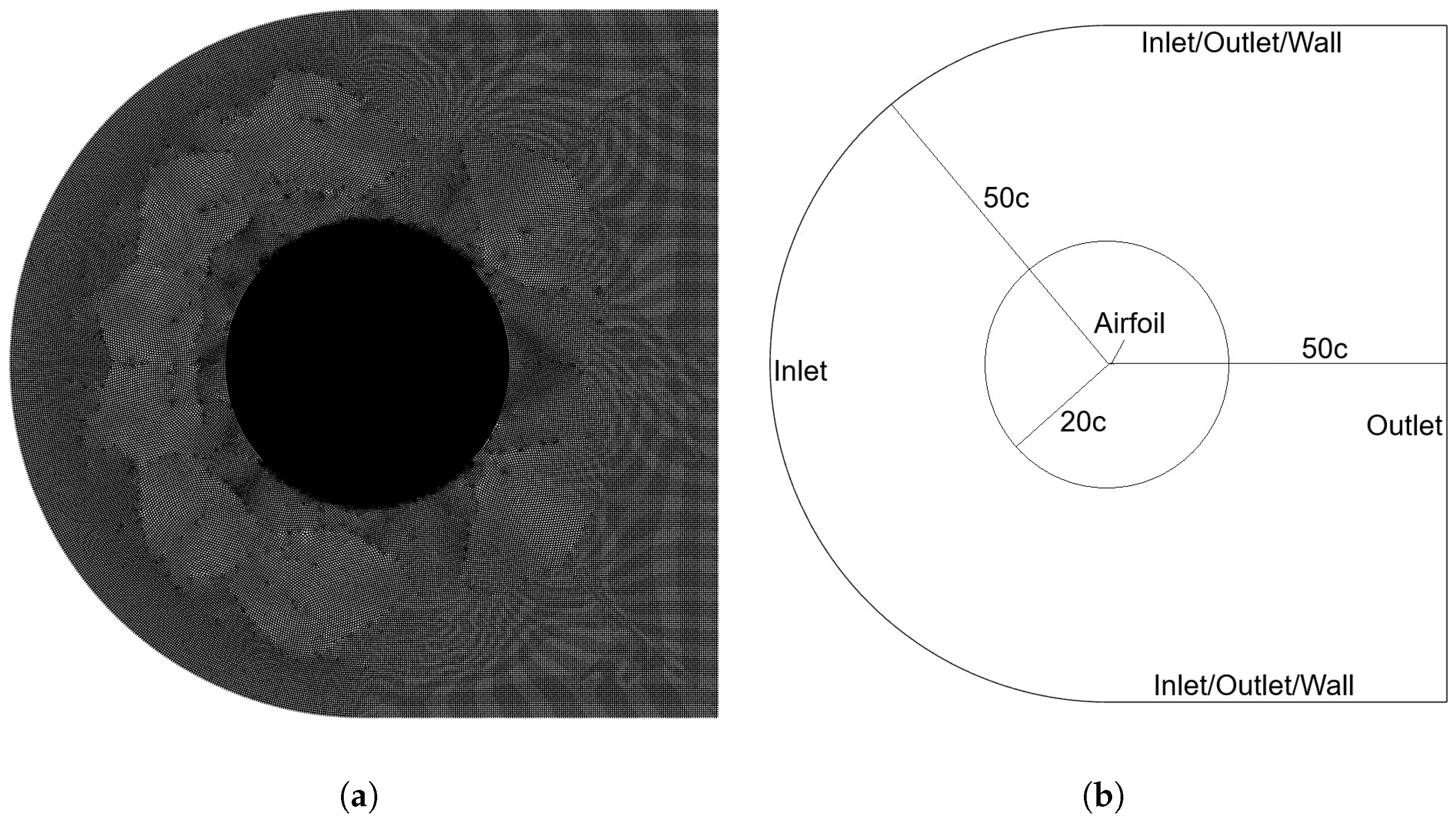
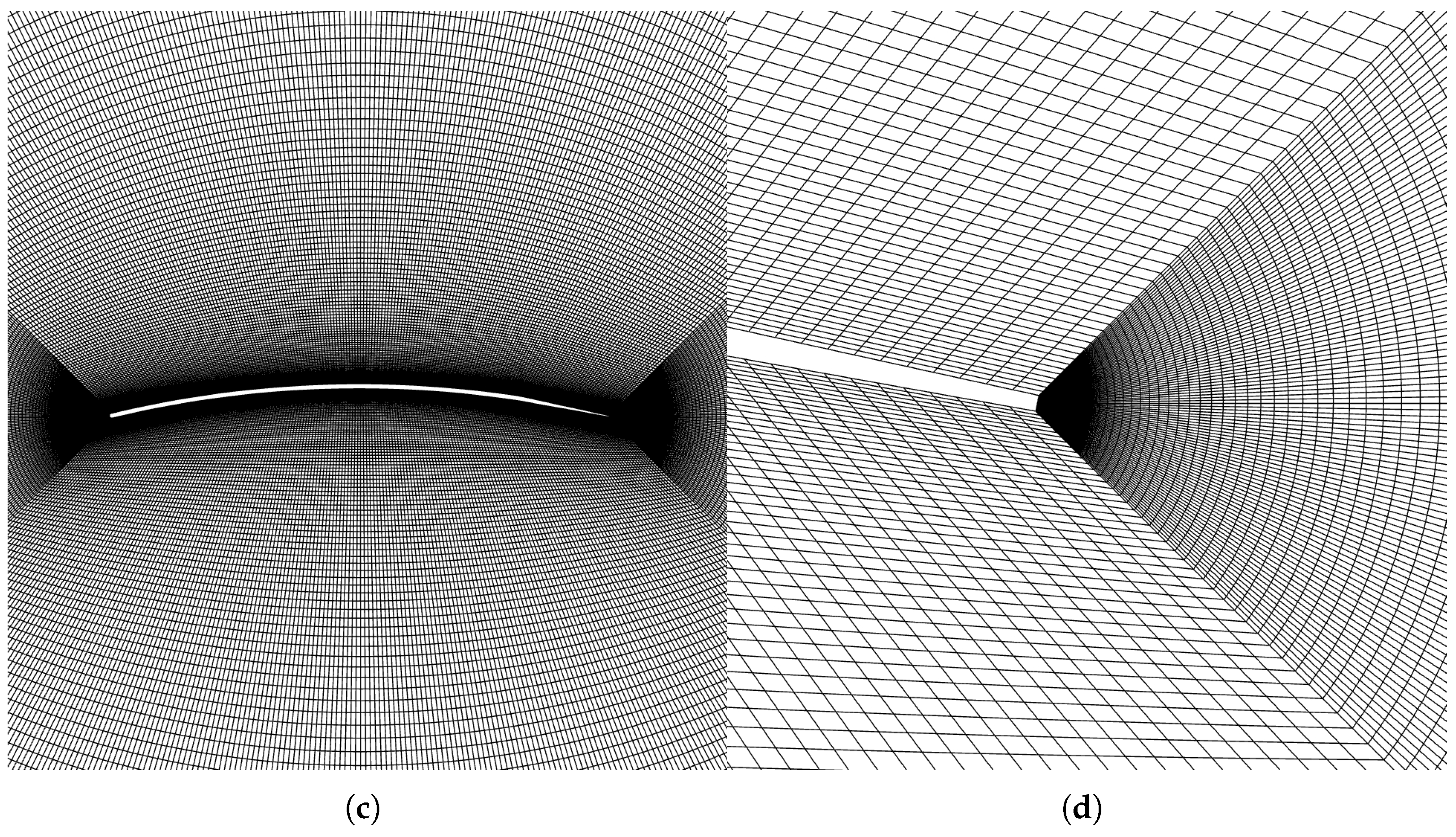
A C-type mesh (Figure 1a) is generated around a cambered plate with 6% camber and 1% thickness over a chord length of 30 mm. Figure 1b shows the computational domain extending 50c in all directions from the airfoil, along with the locations of key boundaries and geometric dimensions. To accurately resolve the boundary layer, mesh clustering is applied in a circular region surrounding the airfoil. Although inflation layers are not used, the near-wall mesh is sufficiently refined to maintain a non-dimensional wall distance of ${\mathrm{y}}^{+}\le 1$. This ensures proper capture of near-wall flow behavior. This localized refinement is visible in Figure 1c. The value of the first cell thickness, the growth rate close to the wall, and the variation of the $y^{+}$ with the angle of attack ($\alpha$) are shown in

Table 1. $y^{+}$ variation with angle of attack, using the same first cell height and growth rate for all cases.

$\mathit{\alpha }$ [°]	Min ${\mathit{y}}^{+}$	Mean ${\mathit{y}}^{+}$	Max ${\mathit{y}}^{+}$	First Cell Height [m]	Growth Rate
0	0.043	0.516	1.679	$4.2\times {10}^{-5}$	1.05
5	0.024	0.526	2.338
8	0.059	0.525	2.332
15	0.072	0.515	2.107

. The maximum values of the $y^{+}$ are always located at the leading edge of the airfoil, where the velocity gradients are highest. Over the rest of the surface, $y^{+}$ remains well within the recommended range. It ensures adequate near-wall resolution for accurately capturing laminar-to-transitional flow behavior. The trailing edge of the airfoil is slightly truncated, as shown in Figure 1d, to approximate the physical geometry used in related experiments. Furthermore, this adjustment improves mesh quality and numerical stability.

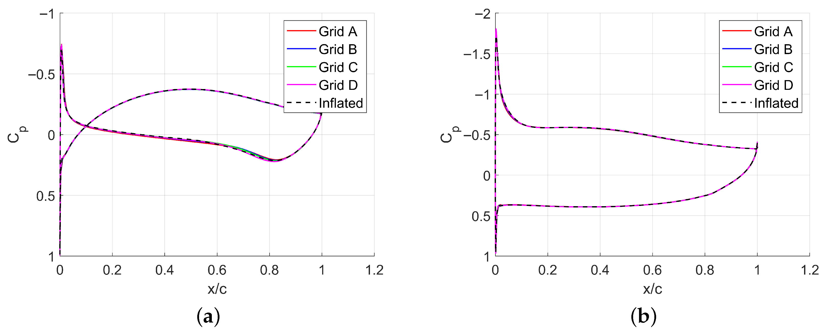
Different grid resolutions are used to conduct a mesh sensitivity study to assess the impact of mesh density on the results using UNS equations. The study includes four meshes: Grid A (200 k elements), Grid B (300 k elements), Grid C (400 k elements), and Grid D (500 k elements), and an additional enlarged mesh. Mesh accuracy is evaluated based on the predicted drag coefficient and the distribution of the pressure coefficient along the surface at two angles of attack, 0° and 5°. As shown in

Table 2. Grid independence study, showing drag coefficients at 0° and 5° and percentage errors relative to Grid B (UNS).

Grid	Elements	${\mathit{C}}_{\mathit{D}}$ 0°	${\mathit{C}}_{\mathit{D}}$ 5°	Error 0° [%]	Error 5° [%]
Grid A	200,000	0.0381663	0.0570116	0.213	0.945
Grid B	300,000	0.0380852	0.0564779	–	–
Grid C	400,000	0.0381419	0.0562283	0.149	0.442
Grid D	500,000	0.0384546	0.0561832	0.969	0.522
Enlarged	700,000	0.0383437	0.0561384	0.679	0.601

, increasing the number of elements beyond Grid B results in a maximum change in the drag coefficient of 0.9% at 0° and 0.52% at 5°. Furthermore, the pressure coefficient distributions on the airfoil surface closely match, with minimal variations between Grids B, C, and D (see Figure 2). Furthermore, the influence of the domain size of the selected mesh is determined by generating an enlarged mesh with double distance between boundaries and the airfoil. This configuration is analyzed using the same criteria to ensure that the placement of the boundaries does not affect the calculations. A minimal drag coefficient change of 0.6% is observed (Table 2). Similarly, the pressure coefficient distributions shows good agreement (see Figure 2).

Grid B, consisting of 300 k elements with domain boundaries located 50c from the airfoil surface, is selected as an optimal mesh. It provides a good balance between accuracy and computational efficiency. This mesh minimizes computational cost while exhibiting minimal deviation compared to results from finer meshes. The mesh quality metrics for Grid B are an average skewness of 0.0538, an average aspect ratio of 1.84, and an average orthogonality of 0.988.

2.3. Boundary Conditions and Settings

The simulations involving the three different models are performed using the same computational setup. This means equal boundary conditions and numerical schemes. Nonetheless, the setups for the RANS models differ on certain parameters, which are adjusted to satisfy their specific requirements. At the same time, they remain as faithful as possible to the experiments.

The domain is divided into four main regions: inlet, outlet, horizontal boundaries, and airfoil surface (see Figure 1b). At the inlet, a uniform velocity profile is applied, corresponding to a Reynolds number of 10,000. Furthermore, the flow direction is adjusted to simulate the different angles of attack. The outlet is defined as a pressure outlet with zero gauge pressure. The horizontal boundaries are defined according to the angle applied to the freestream, used to simulate the different angles of attack of the airfoil. For positive angles, the upper boundary is specified as part of the velocity inlet and the lower boundary of the pressure outlet; for negative angles, the roles are reversed. At $\alpha$ = 0°, both horizontal boundaries are treated as no-slip walls to enforce numerical stability and eliminate artificial inflow/outflow. Finally, the airfoil surface is modeled as a no-slip, smooth wall.

The RANS models employed in this study, namely the $\gamma \text{-}R{e}_{\theta }$ and $k\text{-}{k}_L\text{-}\omega$ models, require specific inlet conditions. Both models expect values for the turbulence intensity (TI) and the turbulent viscosity ratio. Additionally, the $\gamma \text{-}R{e}_{\theta }$ model requires a value for intermittency, while the $k\text{-}{k}_L\text{-}\omega$ model requires the laminar kinetic energy. The turbulence intensity is set to 0.2%, based on the experimental TI, reported to be TI ≤ 0.3% [10]. The turbulent viscosity ratio is set to 1, suggesting a laminar or nearly laminar flow. Intermittency is assigned a value of 0, reflecting the fully laminar nature of the inlet flow. The laminar kinetic energy is specified as $1\times {10}^{-4}$, consistent with the low-turbulence or nearly-laminar flow considered. Additionally, the critical momentum–thickness Reynolds number ($R{e}_{\theta ,c}$) is adjusted to 250 [22], so that it better matches the experimental study. In contrast, the UNS equations do not require any turbulence-related parameters, as no turbulence modeling is involved.

The pressure–velocity coupling is handled using the SIMPLE algorithm. Second-order upwind schemes are employed for all transport equations. Solution initialization is performed with Fluent’s standard initialization procedure, with the inlet boundary as reference. All the other solver controls not specified are left at Fluent’s default values. Furthermore, residuals are monitored through the iterations, but no convergence thresholds are imposed.

2.4. Temporal Resolution

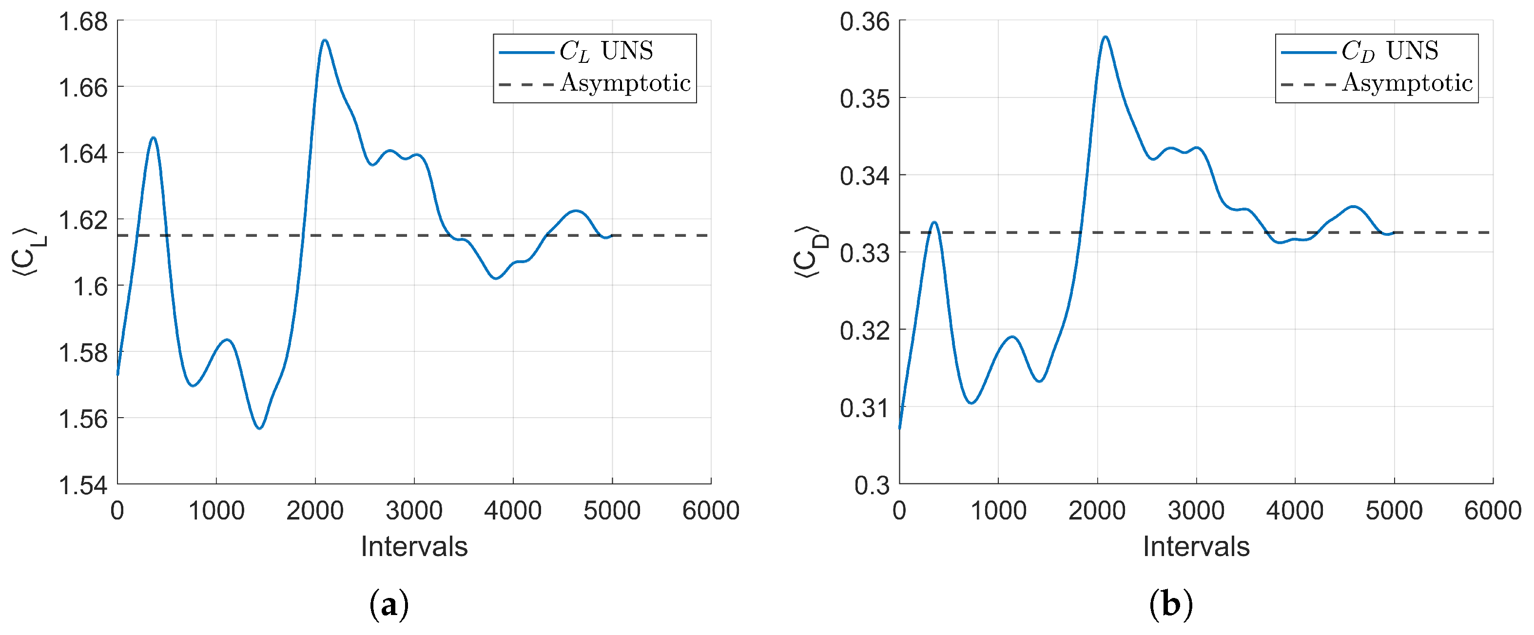
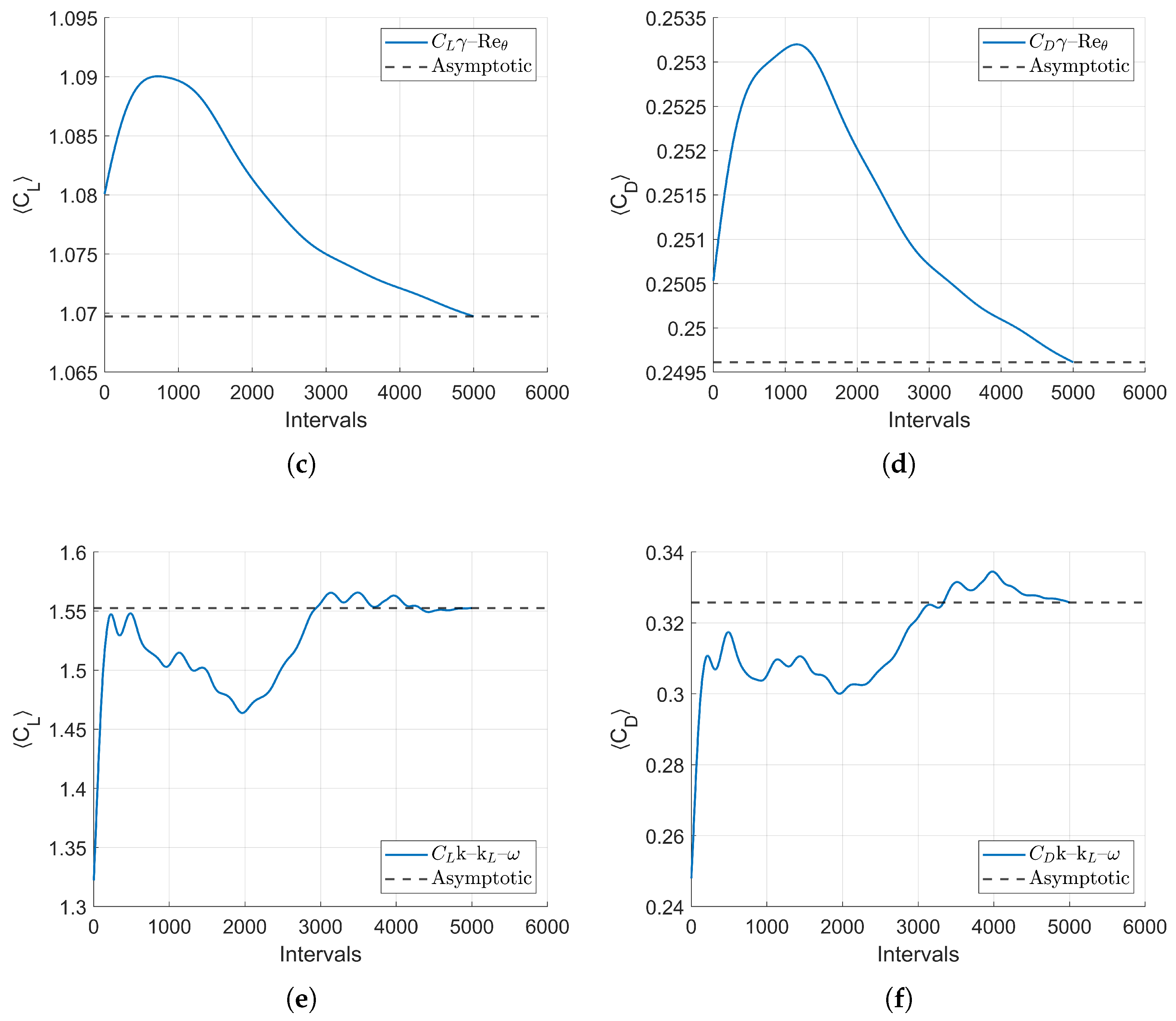
All simulations are conducted using a fixed time step of $1\times {10}^{-5}$ s. This time step ensures temporal accuracy of the unsteady flow. Initial transients are removed so that time-averaged quantities can be computed correctly. More information about the choice of time step and the considered averaging windows is provided in Appendix B.

2.5. Validation

The numerical results are compared with available experimental data from the 1995 study by Okamoto et al. [10], while that paper reviews several experimental investigations, the present work focuses on the study examining the effect of camber on the flow. In the experiments, aluminum foil models were used to replicate cambered plates with 3%, 6%, and 9% camber. Tests were conducted at a Reynolds number of 10,000 with a free-stream turbulence intensity below 0.3%. To ensure reliability in the comparison, the computational setup is designed to match the experimental flow conditions as closely as possible. The geometry adopted in the simulations, consisting of a circular leading edge and a truncated trailing edge, introduces minor geometric differences relative to the experiments. These are not expected to significantly affect the results. Validation is performed across a range of angles of attack covering pre-stall, stall, and post-stall conditions

To assess the level of agreement between the CFD predictions and the experimental observations, the percentage root mean square error (RMSE), mean absolute error (MAE), and maximum absolute error (MaxAE) are calculated for the lift and drag coefficients. MAE indicates typical performance, RMSE highlights larger discrepancies, and MaxAE reveals the worst-case error. Together, they provide a comprehensive characterization of the error, which is important when comparing CFD results and experimental results.

Appendix A presents a detailed assessment of uncertainty and repeatability, reinforcing the robustness of the simulations.

3. Results

This section presents the key aerodynamic results obtained from the unsteady simulations. Due to the unsteady nature of the flow, all data presented are time-averaged values. The analysis focuses on the lift and drag coefficients, comparing results from the three modeling approaches as well as with experimental data [10]. Additionally, the pressure coefficient distributions across the airfoil surface are analyzed.

3.1. Time-Averaged Aerodynamic Coefficients

The lift and drag coefficients over all time steps are collected and averaged to obtain the mean aerodynamic coefficients. The averaging excludes the initial transient phase before the flow reaches a statistically steady state, ensuring more accurate results. At these Reynolds numbers, aerodynamic forces exhibit significant unsteady fluctuations: time-averaged values alone do not fully capture the airfoil’s performance. To provide a more comprehensive understanding, the graphs also include oscillation amplitudes, showing maximum and minimum values along with the standard deviation. Minimum and maximum values are represented by vertical lines, while shaded bands illustrate the standard deviation. Mean and extremes are marked with circular symbols. To improve clarity in the comparisons, data points at the same angle of attack are slightly offset to distinguish overlapping symbols.

Figure 3 shows the lift coefficient for angles of attack ranging from −5° to 15°, calculated with $\gamma$–$R{e}_{\theta }$, $k\text{-}{k}_L\text{-}\omega$ and UNS, compared with the experimental curve [10]. The curves exhibit trends similar to the experimental curve for low angles of attack. For higher angles of attack, the UNS and $k\text{-}{k}_L\text{-}\omega$ models cannot capture the flow behavior and the aerodynamic trend. Experiments show a stall around 10°, which is not predicted by these models. Instead, the lift coefficients continue to increase with a similar trend with increasing angle of attack. Not only do the mean values rise, but the unsteadiness becomes more pronounced, with larger deviations in the maximum, minimum, and standard deviation. Only the $\gamma$–$R{e}_{\theta }$ model captures the decrease in lift coefficient due to stall, which is predicted to occur earlier at 8°. At pre-stall angles, fluctuations in the lift coefficient remain within approximately $\pm 5\%$ of the experimental values for all three models. Beyond stall, only the fluctuations predicted by the $\gamma$–$R{e}_{\theta }$ model decrease, whereas those of the other two models increase to about $\pm 15\%$, indicating greater unsteadiness. Nevertheless, the overall trend remains acceptable and reasonably close to the expected behavior.

Table 3. Error metrics comparing different turbulence models predictions with experimental lift coefficients.

Model	MAE	RMSE	MaxAE
UNS	0.201	0.267	0.605
$\gamma$–$R{e}_{\theta }$	0.067	0.081	0.165
$k\text{-}{k}_L\text{-}\omega$	0.189	0.2444	0.502

summarizes the error metrics, comparing CFD predictions with experimental lift coefficients for the three turbulence models, while the table presents absolute errors, it is important to note that the maximum experimental lift coefficient in the dataset is approximately 1.20.

Similarly, Figure 4 presents the drag coefficient curves predicted by the models alongside experimental data. All models capture the overall trend well, with the $\gamma$–$R{e}_{\theta }$ model showing the closest agreement. Predictions are consistent at low angles of attack, but discrepancies appear beyond the stall near 10°. Around 9°, brief agreement is observed with experiments. Beyond this, the $\gamma$–$R{e}_{\theta }$ model underestimates drag, while the $k\text{-}{k}_L\text{-}\omega$ and UNS models overpredict it, mirroring trends seen in lift coefficient. Moreover, fluctuations in the drag coefficient remain below approximately $\pm 5\%$ of the maximum experimental drag value at pre-stall angles. Post-stall, these fluctuations increase significantly, reaching up to $\pm 20\%$ for the $k\text{-}{k}_L\text{-}\omega$ and UNS models. In contrast, the $\gamma$–$R{e}_{\theta }$ model exhibits a marked reduction in drag fluctuations beyond stall, with variability decreasing to nearly negligible levels. Overall, drag predictions are more consistent across models than lift, reflected in the error metrics shown in

Table 4. Error metrics comparing different turbulence models predictions with experimental drag coefficients.

Model	MAE	RMSE	MaxAE
UNS	0.023	0.029	0.088
$\gamma$–$R{e}_{\theta }$	0.018	0.019	0.035
$k\text{-}{k}_L\text{-}\omega$	0.020	0.025	0.055

. Similarly to the error analysis performed for the lift coefficient, this table presents the absolute errors, which give important information considering the maximum experimental drag coefficient to be 0.272.

To complete the aerodynamic analysis, Figure 5 shows the lift-to-drag ratio ($C_L$/$C_D$), representing aerodynamic efficiency across angles of attack. All models reproduce a similar overall shape to the experimental curve, qualitatively capturing the efficiency trend. However, simulations overestimate efficiency, with peak values near 15, compared to the experimental maximum just above 10. The model curves closely match between 0° and 8°, consistent with lift and drag results. After stall, predicted at 8° by the $\gamma$–$R{e}_{\theta }$ model, efficiency drops and aligns with experiments. In contrast, the $k\text{-}{k}_L\text{-}\omega$ and UNS models, which miss the stall, continue to overpredict $C_L$/$C_D$ beyond this point.

3.2. Time-Averaged Pressure Coefficient Distributions

Although the experimental pressure coefficient ($C_p$) distributions are not available, the simulated $C_p$ curves are analyzed and compared. These provide valuable insights into the aerodynamic behavior predicted by the models, particularly regarding flow separation and possible transition. This analysis helps interpret the trends observed in the lift and drag coefficients, offering an additional level of comparison across the models. The focus is placed on the suction surface of the airfoil. It is worth noting that, for negative angles of attack, an LSB forms on the pressure surface, but this is not central to the current analysis. As with the other coefficients, the pressure coefficients are collected and averaged over the time steps to account for oscillations present in some models and at certain angles of attack. These distributions illustrate the pressure variation along the entire chord of the airfoil, from the leading to the trailing edge. Only selected angles of attack, representative of key aerodynamic conditions, are shown below.

The good agreement between models at pre-stall and stall angles indicates that flow behavior is captured similarly, including the formation of an LSB at both 7° and 8°. At these angles, the plateau and peak in the pressure distribution signal the presence of the LSB, which clearly increases in size at the higher angle, as seen in Figure 6b,c. Figure 6d shows the $C_p$ distribution at 13°, confirming the divergence among the models after stall. The $\gamma$–$R{e}_{\theta }$ model predicts complete flow separation after 8°, as indicated by the flattening of the curve following the leading-edge peak. This behavior corresponds to stall, caused by the burst of the LSB. In contrast, the $k\text{-}{k}_L\text{-}\omega$ model and the UNS equations continue to predict a growing LSB with turbulent reattachment, without showing signs of stall. The persistence and increasing size of the LSB explain the continued rise of the lift coefficient observed in Figure 3.

3.3. Computational Performance

To complement the aerodynamic performance comparison,

Table 5. Total simulation time for each model.

Model	Average Time	Standard Deviation
	[hh:mm:ss]
UNS	04:35:47	00:02:54
$\gamma$–$R{e}_{\theta }$	07:13:15	00:02:27
$k\text{-}{k}_L\text{-}\omega$	07:13:00	00:03:01

reports the average clock time for each model used. These values represent the time required to complete a simulation for one angle of attack, run on 48 cores in ANSYS Fluent.

4. Discussion

The results presented in the previous section highlight key differences between the models in their ability to predict the correct flow behavior.

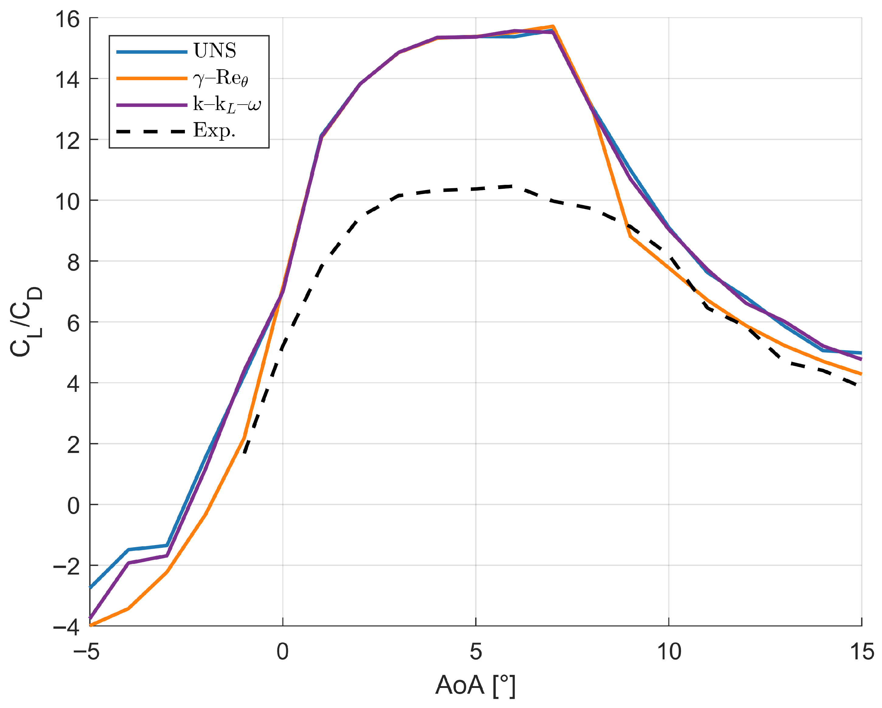
The most evident discrepancy lies in the prediction of the lift coefficient and stall behavior, as shown in Figure 3; while none of the models perfectly reproduce the experimental lift values, the $\gamma$–$R{e}_{\theta }$ model demonstrates superior predictive capabilities. It is the only model that captures stall, even if predicting its onset at around 8°, compared to the experimental 10°. This improved performance is attributed to its incorporation of intermittency and momentum–thickness Reynolds number transport equations. These features enable a more accurate representation of transitional phenomena and LSB formation. The inability of the $k\text{-}{k}_L\text{-}\omega$ and UNS models to predict stall reveals their limitations in modeling transitional effects. Although the $k\text{-}{k}_L\text{-}\omega$ model is specifically designed for transition prediction, it is highly sensitive to initial conditions and empirical correlations. At low Reynolds numbers, such as $Re$ = 10,000, these correlations may not accurately represent natural transition. Consequently, this leads to inaccurate transition prediction and poor lift estimation near and beyond stall. The UNS equations, lacking any turbulence modeling, are unable to predict transition or turbulent behavior. Despite this, the UNS model performs reasonably well at low angles of attack, where the flow remains predominantly laminar. However, without a mechanism to capture transition, it fails to predict stall and unrealistically shows a continuous increase in lift with angle of attack. These conclusions are supported by the absolute errors that are presented in Table 3. It is clear that $\gamma$–$R{e}_{\theta }$ has the lowest MAE, RMSE, and MaxAE, showing that it outperforms the other models with more accurate and consistent predictions. The UNS and $k\text{-}{k}_L\text{-}\omega$ models exhibit similar performance, with higher errors and larger maximum deviations, i.e., less reliability in capturing lift behavior.

The drag coefficient predictions (Figure 4) reveal consistent trends across all models, with divergence becoming more evident at higher angles of attack. The $\gamma$–$R{e}_{\theta }$ model predicts lower drag coefficients, indicating fully separated flow. In contrast, the $k\text{-}{k}_L\text{-}\omega$ and UNS models continue to capture a growing LSB, resulting in higher drag values. Despite this, the predictions remain reasonably accurate even after stall, showing less pronounced deviations from the experimental data compared to lift coefficients. This behavior can be attributed to the drag coefficient’s lower sensitivity to turbulence modeling, as it is primarily influenced by viscous skin-friction forces. Once again, the superior performance of the $\gamma$–$R{e}_{\theta }$ model is demonstrated by the consistently lowest errors reported in Table 4. The comparatively lower precision and greater deviations observed in the other models are further confirmed.

The lift and drag results reveal each model’s ability to capture stall and transitional behavior, which is crucial for design considerations. Accurate stall prediction is fundamental for small UAV and MAV design. Underestimating maximum lift or overestimating efficiency could directly affect payload capacity, endurance, and control stability; while the $\gamma$–$R{e}_{\theta }$ model provides the most accurate stall predictions, its sensitivity to empirical parameters limits robustness without careful tuning. In contrast, the UNS equations, despite lacking turbulence modeling, offer reliable pre-stall predictions at a fraction of the computational cost, making them suitable for preliminary trend identification. The $k\text{-}{k}_L\text{-}\omega$ model, however, shows neither superior accuracy nor efficiency, suggesting limited applicability for this regime. These findings highlight the importance of balancing predictive accuracy and computational cost when selecting models for design studies and underscore the need for continued refinement of transition modeling approaches at low Reynolds numbers.

Another important aspect to consider is the unsteady nature of the flow and the role of LSBs. These bubbles play a critical role in determining the accuracy of each model’s predictions. It is also important to recognize that the truncated trailing edge of the airfoil contributes to the observed oscillations, and this effect should be taken into account. However, geometry-induced oscillations tend to be more regular, whereas the unsteady variations observed here are primarily caused by the transitional behavior of the flow. Furthermore, the magnitude of these fluctuations depends significantly on the model used and its capability to capture transitional and unsteady flow phenomena. At pre-stall angles, fluctuations in both lift and drag coefficients remain relatively low across all models. However, beyond stall, unsteadiness increases significantly for the $k\text{-}{k}_L\text{-}\omega$ and UNS models, highlighting their difficulty in predicting the dynamics of the separated flow. 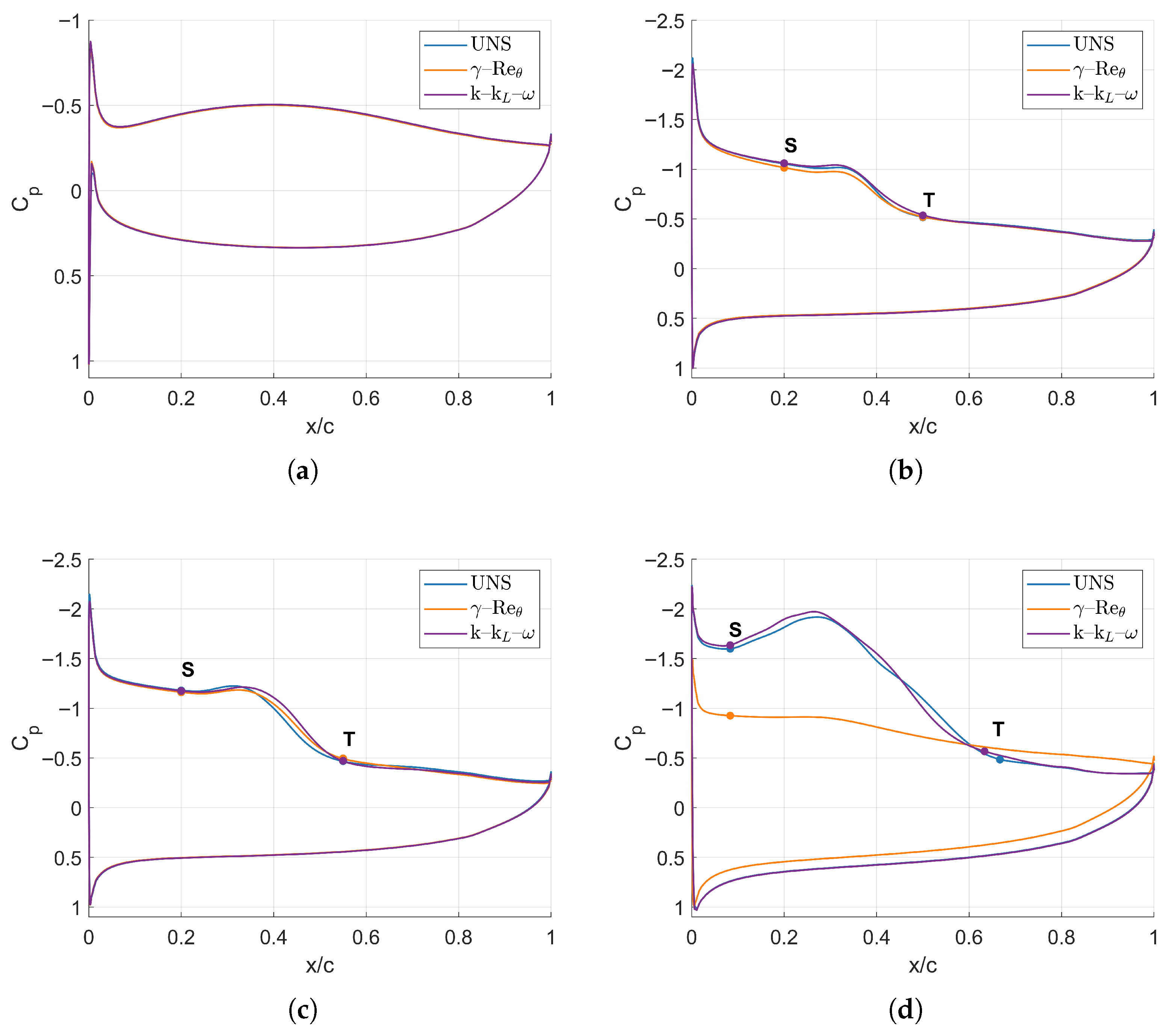In contrast, the $\gamma$–$R{e}_{\theta }$ model shows a marked reduction in post-stall oscillations. This improved performance is tied to its ability to capture the formation and evolution of LSBs, although it does so slightly prematurely. The characteristic plateau and suction peak associated with LSBs are clearly visible in its pressure coefficient distributions (Figure 6); while the other models can also predict LSBs, they consistently fail to capture their bursting and the resulting stall, as confirmed by the persistent lift overprediction and absence of pressure recovery in post-stall conditions.

From a practical standpoint, the choice of turbulence model should be guided by both the type of flow and the purpose of the analysis. For pre-stall angles, where the flow is largely laminar, the UNS equations provide sufficiently accurate predictions. They require significantly less computational effort, making UNS ideal for preliminary design studies aimed at capturing general flow trends. However, UNS is not suitable for comprehensive analyses, as the lack of turbulence modeling prevents it from accurately predicting stall and post-stall behavior. The $k\text{-}{k}_L\text{-}\omega$ model, while intended for transition prediction, shows results very similar to UNS in this low Reynolds-number regime. Its accuracy is highly sensitive to inlet conditions and empirical correlations, and at $Re$ = 10,000 it fails to provide reliable stall and post-stall predictions. Based on the present study, this model appears unsuitable, and it is unclear whether adjustments could significantly improve its performance. In contrast, the $k\text{-}{k}_L\text{-}\omega$ model has been shown to be effective in higher Reynolds number regimes, where its empirical correlations are more valid. A comprehensive sensitivity study of $k_L$ initialization and inlet parameters would be required to fully assess robustness at these low-$Re$ regimes, which is beyond the scope of the present work. The $\gamma$–$R{e}_{\theta }$ model, despite its higher computational cost, provides the most accurate predictions among the three; while it captures stall and post-stall behavior well, empirical correlations cause a slight early stall prediction, highlighting the need for careful calibration.

5. Conclusions

This paper presents a comparison between two RANS turbulence models, $\gamma$–$R{e}_{\theta }$, $k\text{-}{k}_L\text{-}\omega$, and the UNS equations, evaluating their ability to predict flow behavior at a Reynolds number of 10,000. The simulation results are compared with experimental data obtained from flow over a thin airfoil with 6% camber and 1% thickness. The accuracy of the models is assessed based on aerodynamic coefficients. Pressure coefficient distributions are also analyzed to further support the conclusions.

The analysis reveals that none of the three models perfectly capture the flow physics at this low Reynolds number, although all can reproduce the overall trends in lift and drag coefficients. The $\gamma$–$R{e}_{\theta }$ model performs best, successfully capturing the presence of LSBs and predicting stall onset, although earlier than observed experimentally. Figure 3 and Figure 6 show that the other two models fail to predict stall. Instead, they indicate a continuous increase in lift coefficient and an unsteady but growing LSB that never bursts. These conclusions are supported by the pressure coefficient distributions, particularly at 13°, where the total flow separation predicted by $\gamma$–$R{e}_{\theta }$ contrasts with the persistent LSB predicted by the other two models.

Accurate stall prediction is essential for reliable estimation of aerodynamic performance and ensuring safe airfoil operation. On the one hand, the UNS equations perform better than expected, predicting the general trend with acceptable error levels for low angles of attack, while requiring significantly less computational time. The use of UNS equations at this Reynolds number is therefore a viable and efficient choice for preliminary studies aimed at trend identification. This finding aligns with previous work by Koning et al. [16]. On the other hand, while the $k\text{-}{k}_L\text{-}\omega$ model is designed for transition prediction, its application at low Reynolds numbers is hindered by high sensitivity to empirical correlations and initial conditions, complicating accurate transition and stall prediction. The $\gamma$–$R{e}_{\theta }$ model also relies heavily on empirical parameters, such as $R{e}_{\theta }$. Nevertheless, it performs well in capturing key transitional features like LSBs and predicting stall, albeit slightly early.

Although validation data are limited to the experimental study of Okamoto [10], several factors support the reliability of this analysis. Observed aerodynamic trends, such as stall onset, LSB development, and post-stall behavior, align with previous experimental and numerical studies at comparable Reynolds numbers [5,6,9]. Using three different modeling approaches under identical conditions enables systematic cross-comparison. Simultaneously, mesh independence and boundary condition sensitivity checks ensure the results are not numerical artifacts. Together, these points provide confidence in the conclusions despite the scarcity of detailed experimental benchmarks. Nevertheless, new experimental datasets would be highly valuable. In particular, more detailed information on setup parameters and flow characteristics would support improved model initialization and, consequently, greater predictive accuracy. Furthermore, measurements of pressure coefficient distributions would enable direct comparison with simulations, allowing for a more comprehensive validation of the models.

In summary, the three models demonstrate varying capabilities in predicting transitional flow features. This highlights the importance of selecting the appropriate approach based on the flow regime and study objectives. The $\gamma$–$R{e}_{\theta }$ model generally offers the most reliable results, capturing stall and post-stall behavior with good agreement. However, it requires careful tuning of empirical parameters and initial conditions to maximize accuracy. The $k\text{-}{k}_L\text{-}\omega$ model also requires tuning, but its reliance on empirical correlations makes it unsuitable for low Reynolds number flows, as seen in this study. The UNS model emerges as an efficient option for early-stage investigations or preliminary design studies, where computational resources or time are limited and extreme precision is not critical. Ultimately, ongoing refinement and calibration of turbulence and transition models remain essential to improve the accuracy of low Reynolds number simulations. From a practical standpoint, UNS is recommended for efficient pre-stall trend estimation, $\gamma$–$R{e}_{\theta }$ for accurate stall and post-stall performance, and $k\text{-}{k}_L\text{-}\omega$ is less suitable in this low-$Re$ regime due to poor robustness and sensitivity to setup parameters.