Adaptive Disturbance Rejection Generalized Predictive Control of Photoelectric Turntable Servo System

Abstract

In order to enhance the tracking accuracy and disturbance rejection capability in the speed loop of an optoelectronic tracking servo control system, a parameter self-adjusting disturbance rejection generalized predictive control method (STGPC) based on a continuous-time model is proposed in this paper. First, a dynamic model of the servo turntable system is established, and a linear extended state observer (LESO) is designed to perform real-time estimation of internal and external disturbances in the system. Second, a generalized predictive control law incorporating the predictive model, performance metrics, and rolling optimization is systematically derived, where the reference trajectory is generated by a tracking differentiator and the system state is provided in real time by the LESO. Furthermore, a gradient descent method is innovatively introduced to achieve adaptive adjustment in the predictive time domain, and the stability of the closed-loop system is rigorously proven based on Lyapunov theory. Finally, simulation experiments were conducted to verify the tracking performance, disturbance rejection performance, and time-domain parameter self-adjustment effects of the control method. Simulation results show that compared with PID control and traditional linear generalized predictive control (LGPC), the proposed STGPC method reduces speed tracking residuals by 73.79% and 51.04%, respectively, enhances disturbance suppression capability for speed vibration disturbances by 50.55% and 47.55%, respectively, and enhances compensation capability for friction torque disturbances by 68.03% and 59.33%, respectively. The system demonstrates outstanding velocity tracking accuracy and disturbance rejection while exhibiting good robustness against system parameter perturbations.

1. Introduction

With the development of industrial and electronic technologies, the requirements for tracking accuracy, response time, and interference resistance of servo turntable control in optoelectronic tracking systems are becoming increasingly stringent [1]. The speed loop of traditional optoelectronic servo systems still primarily relies on PID control. This method is constrained by the system architecture and effective signal bandwidth, limiting the design of control parameters [2]. There is room for further improvement in the system’s disturbance rejection capability and control accuracy, making it necessary to explore advanced control algorithms suitable for optoelectronic servo turntables.

With the enhanced computational capabilities of embedded systems today, devices are now capable of implementing advanced control algorithms such as optimal control [3], sliding mode control [4], and predictive control [5,6]. Among these, generalized predictive control [7] (GPC) stands out for its superior control performance. Originating from practical industrial applications, GPC holds significant engineering reference value. In [8], the authors construct a linear model generalized predictive control (LGPC) using a continuous-time predictive model, avoiding complex calculations and making the implementation of GPC in servo control feasible. In [9], the authors construct a fractional-order cost function to enhance the control performance of GPC. In [10], the authors implemented adaptive adjustment of the predictive time domain of GPC, enhancing the versatility of the controller. In [11], the authors proposed a novel composite generalized dynamic predictive control. By introducing a self-tuning horizon mechanism, it enables autonomous and dynamic adjustment of the prediction horizon across diverse speed regulation ranges, resulting in significantly improved performance optimization compared to the conventional GPC method. In [12], the authors presented an innovative solution that ingeniously combines an antisaturation extended state observer and an enhanced generalized predictive controller to improve servo control performance, particularly when the system operates in saturated conditions.

In the engineering practice of control algorithms, the handling of disturbances directly affects the final control performance. In [13], the authors identified the model of a large-aperture fast steering mirror and designed a predictive controller based on this model, thereby improving the system’s disturbance rejection capability. In [14], the authors employed a high-order extended state observer (ESO) to compensate for lumped disturbances in the system, thereby enhancing the disturbance rejection capability of the GPC. In [15], the authors combined a high-order sliding mode observer with a predictive controller to improve the system’s disturbance rejection capability. These studies provide insights for enhancing the disturbance rejection performance of GPCs. In [16], the authors modified the command filtered control to address tracking and synchronization issues in dual-motor servo mechanisms and developed an enhanced extended state observer to estimate lumped disturbances. In [17], the authors proposed an improved active disturbance rejection control based on state feedback compensation, improving the accuracy of the turntable servo system, and improved the robustness of the system under nonlinear friction conditions.

To improve the performance of the speed loop in the optoelectronic tracking system, this paper proposes a novel self-tuning disturbance-resistant generalized predictive control strategy based on an optoelectronic servo turntable. By designing the ESO based on the system model, the required state variables for updating the system’s predicted output are provided while observing the lumped disturbance. By designing the time-domain parameter update formula based on control residuals, self-tuning of parameters within a certain range is achieved. Compared with existing optoelectronic servo turntable control schemes, the main contributions of this paper can be summarized as follows:

• Linear generalized predictive control is derived for optoelectronic turntables, combining an extended state observer and a tracking differentiator to calculate the control law, thereby improving the control accuracy and disturbance rejection capability of the optoelectronic tracking turntable speed loop.
• The gradient descent [18] concept is introduced into the parameter tuning of traditional linear generalized predictive control, enabling the system to have a certain degree of parameter self-adjustment capability.

2. System Model Analysis

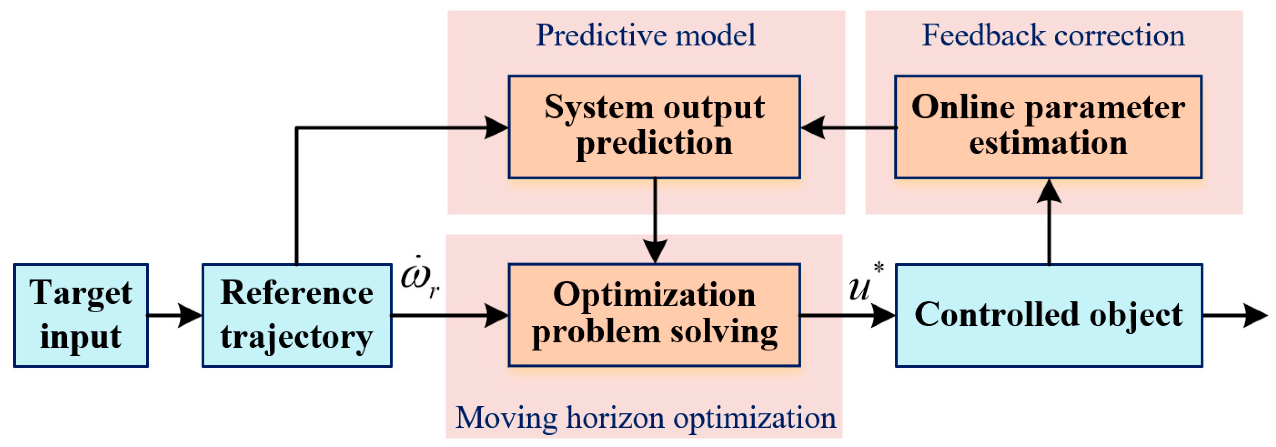
The general predictive control algorithm can be divided into three parts: predictive model, rolling optimization, and feedback correction. The structure of the control system is shown in Figure 1. In the figure, the prediction model is responsible for predicting the future state of the system based on the model and the current state. Rolling optimization combines the output of the prediction model and the reference trajectory to solve the local optimal problem and provide the current optimal control law. Feedback correction updates the model in real time, providing reliable input to the prediction model, forming a closed-loop system for the entire GPC system. The three major parts are interdependent.

Due to the high real-time requirements for control strategies in servo systems, to facilitate the implementation of GPC on an optoelectronic turntable, we refer to the LGPC form and use the Taylor series expansion of the system output to obtain a prediction model. For real-time calculation of the predicted values, a detailed analysis of the controlled object is required to derive the turntable state equations. This part will be explained in detail below.

2.1. Controller Model

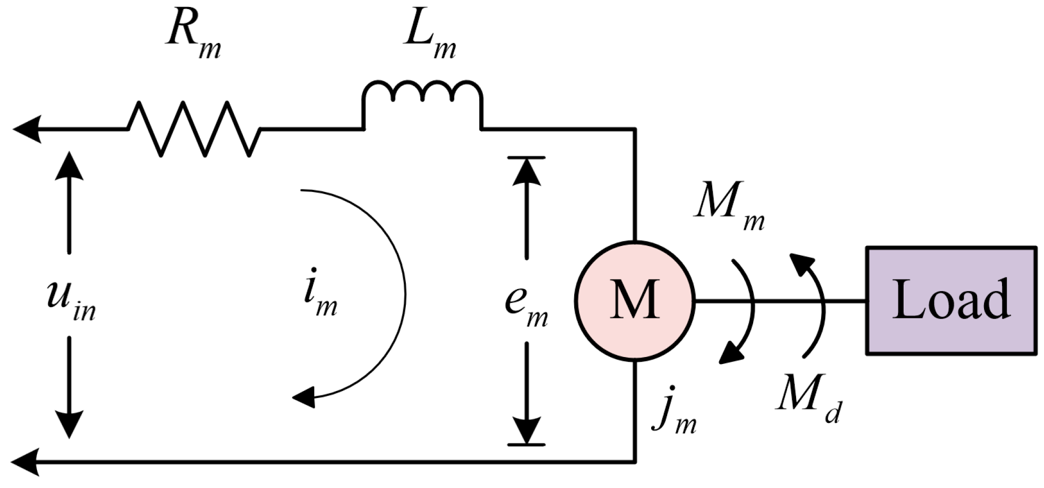
For convenience of derivation, the controlled turntable is approximated as a permanent magnet DC torque motor. Considering the interference torque on the torque motor during operation, the motor load model is shown in Figure 2.

In Figure 2, u_in is the voltage across the armature terminals, i_m is the armature current, L_m is the inductance of the armature winding, R_m is the resistance of the armature winding, e_m is the counter-electromotive force acting on the motor, j_m is the rotational inertia of the motor, M_m is the output torque of the motor, and M_d is the sum of the disturbance torques acting on the motor.

According to electrical and dynamic principles, the voltage balance equation can be obtained as

$$u_{in}(t)=L_m{\displaystyle \frac{d{i}_m(t)}{dt}}+R_m{i}_m(t)-e_m$$

(1)

The motor torque balance equation is

$$M_m(t)=j_m{\displaystyle \frac{d{\omega }_m(t)}{dt}}+M_d$$

(2)

The motor output torque and back EMF equations are

$$M_m(t)=C_m{i}_m(t)$$

(3)

$$e_m=C_e{\omega }_m(t)$$

(4)

where ω_m is the angular velocity of the motor rotor, C_m is the motor torque constant, and C_e is the back EMF constant.

From Equations (2) and (3), we can conclude that

$$i_m(t)={\displaystyle \frac{1}{C_m}}\left(j_m{\displaystyle \frac{d{\omega }_m(t)}{dt}}+M_d\right)$$

(5)

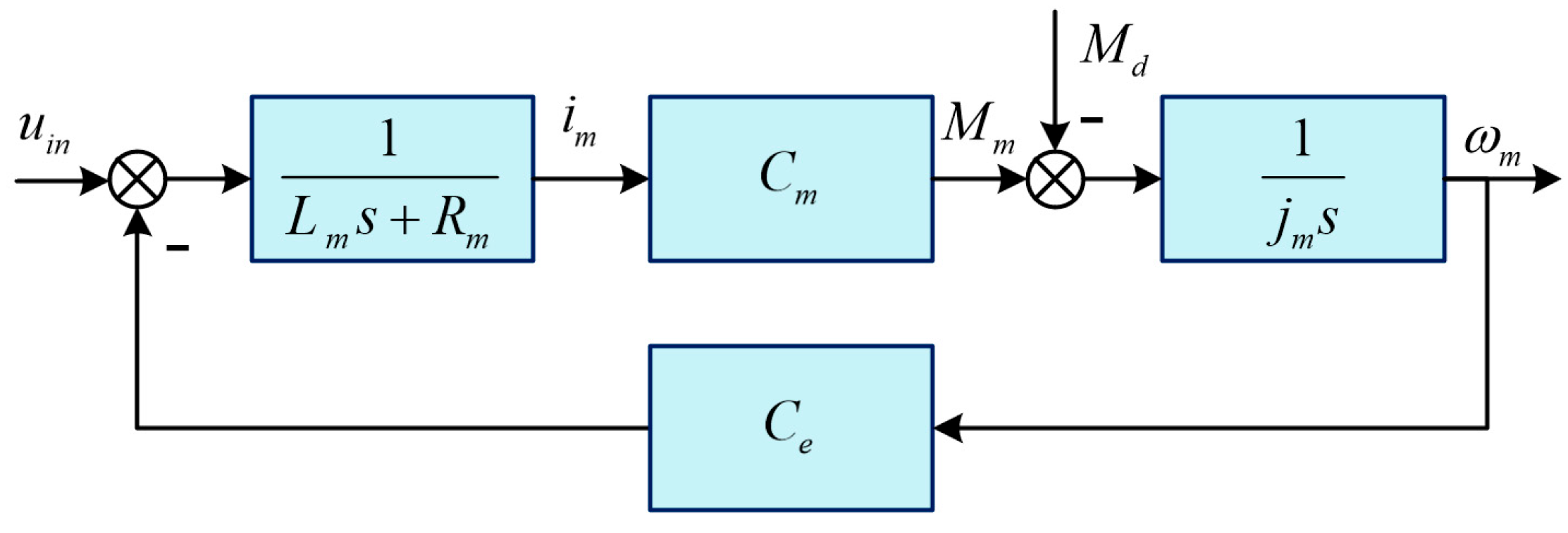
Based on the above analysis, the block diagram of the permanent magnet DC torque motor model is shown in Figure 3.

Temporarily ignoring the disturbance torque M_d, combining Equations (1), (4) and (5), we obtain the relationship between the time-domain speed and input voltage of a permanent magnet DC torque motor as follows

$$u_{in}={\displaystyle \frac{j_m{L}_m}{C_m}}{\ddot{\omega }}_m+{\displaystyle \frac{j_m{R}_m}{C_m}}{\dot{\omega }}_m-C_e{\omega }_m$$

(6)

From Figure 3, we can obtain the velocity change ω_d caused by the disturbance torque M_d:

$${\omega }_d=k_1{\ddot{\omega }}_d+k_2{\dot{\omega }}_d-{\displaystyle \frac{k_1}{j_m}}{\dot{M}}_d-{\displaystyle \frac{k_2}{j_m}}{M}_d$$

(7)

where $k_1=j_m{L}_m/C_m{C}_e$, $k_2=j_m{R}_m/C_m{C}_e$, and ω_d is the velocity change caused by the disturbance term.

The paper mainly focuses on the design of the speed loop. To facilitate the construction of a generalized predictive controller, combining Equations (6) and (7), the superposition theorem can be used to obtain the expression for ω_m as follows

$${\ddot{\omega }}_m=-{\displaystyle \frac{k_2}{k_1}}{\dot{\omega }}_m^{*}+{\displaystyle \frac{1}{k_1}}{\omega }_m^{*}+\delta +k_3{u}_{in}$$

(8)

where $k_3=1/C_e{k}_1$ is the control coefficient, ${\dot{\omega }}_m^{*}={\dot{\omega }}_m+{\dot{\omega }}_d$ is the acceleration after the disturbance torque acts, ${\omega }_m^{*}={\omega }_m+{\omega }_d$ is the velocity after the disturbance torque acts, and $\delta ={\displaystyle \frac{1}{j_m}}{\dot{M}}_d+{\displaystyle \frac{R_m}{L_m{j}_m}}{M}_d$.

Based on the above analysis, both the velocity and acceleration components contain portions caused by disturbances. The state equation of the torque motor system velocity loop can be written as follows

$$\left\{\begin{array}{l}{\dot{x}}_1=F_1+x_2\hfill \\ {\dot{x}}_2=F_2+k_3{u}_{in}\hfill \\ y=x_1\hfill \end{array}\right.$$

(9)

where $x_1={\omega }_m$, $x_2={\dot{x}}_1$, $F_1={\dot{\omega }}_d$, and $F_2=-(k_2/k_1){\dot{\omega }}_m^{*}+(1/k_1){\omega }_m^{*}+\delta$.

In the state equation (Equation (9)), the disturbance quantities F₁ and F₂ have an adverse effect on the control system, but it is difficult to compensate for them directly through sensor measurements. Therefore, F₁ and F₂ are combined into higher-order states and treated as lumped disturbances to design a state observer.

2.2. State Observation Model

Combining Equation (9), the states to be observed are designed as follows

$$\left\{\begin{array}{l}{\dot{z}}_1=z_2\hfill \\ {\dot{z}}_2=k_3{u}_{in}+z_3\hfill \\ {\dot{z}}_3=\dot{F}\hfill \end{array}\right.$$

(10)

where $z_1={\omega }_m$, $z_2={\dot{\omega }}_m$, and $z_3=F$.

The new state z₃ expanded from the original system by the observer is the system’s lumped disturbance. We now propose Hypothesis 1.

Hypothesis 1.

Combining the expression of the system’s lumped disturbance F, we assume that F can be equivalently represented as a polynomial-type disturbance with respect to time t. Therefore, the finite-order derivatives of the lumped disturbance F with respect to time t should exist, and the highest-order derivative should be a constant C. If the terms ${\dot{\omega }}_m^{*}$ and $\delta$ in the hypothesis expression do not have higher-order derivatives and ${\omega }_m^{*}={\dot{\omega }}_m^{*}t$, then the first-order derivative of F is the constant C.

Hypothesis 1 implies that the energy of the lumped disturbance F is finite [19] and can be estimated using the observer.

Combining Hypothesis 1 with Equation (10), the linear ESO is obtained as follows

$$\left\{\begin{array}{l}{e}_1={\widehat{z}}_1-z_1\hfill \\ {\widehat{\dot{z}}}_1={\widehat{z}}_2-{\beta }_{01}{e}_1\hfill \\ {\widehat{\dot{z}}}_2={\widehat{z}}_3-{\beta }_{02}{e}_1+k_3{u}_{in}\hfill \\ {\widehat{\dot{z}}}_3=-{\beta }_{03}{e}_1\hfill \end{array}\right.$$

(11)

where ${\widehat{z}}_1$, ${\widehat{z}}_2$, and ${\widehat{z}}_3$ are the observed values of states $z_1$, $z_2$, and $z_3$, respectively, and ${\beta }_{01}$, ${\beta }_{02}$, and ${\beta }_{03}$ are the observer gains.

Let $e_1={\widehat{z}}_1-z_1$, $e_2={\widehat{z}}_2-z_2$, and $e_3={\widehat{z}}_3-z_3$. Combining this with Equation (11), we obtain the observer state error equation as follows

$$\dot{e}=A_{e}e+B_e\zeta$$

(12)

where $A_e=\left[\begin{array}{ccc}-{\beta }_{01}& 1& 0\\ -{\beta }_{02}& 0& 1\\ -{\beta }_{03}& 0& 0\end{array}\right],B_e={\left[0,0,-1\right]}^T$, $e={\left[e_1,e_2,e_3\right]}^T$, and $\zeta =\dot{F}$.

To ensure the normal operation of the observer, the bandwidth configuration method is used to set the parameter β [20], and the characteristic equation of A_e is

$${\lambda }^3+{\beta }_{01}{\lambda }^2+{\beta }_{02}\lambda +{\beta }_{03}=(\lambda -{\omega }_b{)}^3$$

(13)

Therefore, when the parameters are selected as ${\beta }_{01}=3{\omega }_b$, ${\beta }_{02}=3{\omega }_b^2$, and ${\beta }_{03}={\omega }_b^3$, the observation error is Hurwitz stable.

3. Improved Generalized Predictive Controller

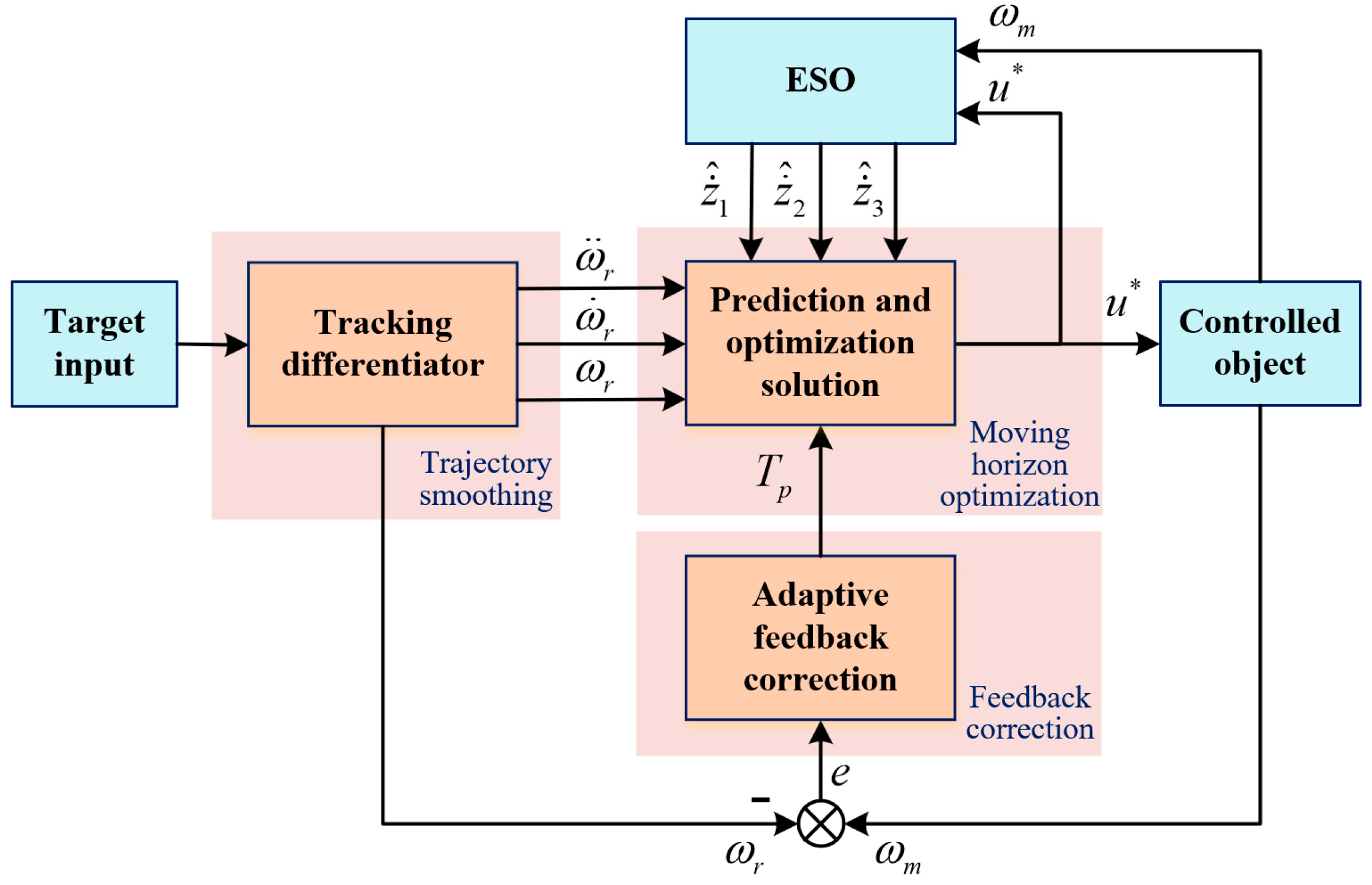
In the model analysis of the previous section, the system state expressions required for GPC design were obtained. Figure 4 shows the structure diagram of the improved generalized predictive controller. In this section, the specific forms of the predictive model, softened trajectory, performance metrics, and rolling optimization solution will be presented based on Figure 4.

3.1. Speed Prediction Model

In predictive control, the predictive model directly determines the final control accuracy. Traditional GPC uses the CARIMA [21] predictive model, which results in a large amount of computation that is detrimental to the real-time performance of the servo system. Therefore, GPC is designed based on a continuous predictive model, using a Taylor series expansion of the speed output ω_m for prediction.

Generally, the higher the order of the predictive model, the higher the prediction accuracy. However, in actual systems, increasing the order can cause the following two problems: it can burden the real-time performance of the control level, and it can be difficult to obtain the higher-order derivatives of the system state.

The selection of the expansion order is generally related to the system order [22]. From Equation (8), it can be seen that the highest order of the controlled system is 2. Therefore, a second-order Taylor expansion is performed on the prediction quantity ω_m, resulting in the following prediction model:

$${\omega }_m(t+\tau )={\omega }_m(t)+\tau {\dot{\omega }}_m(t)+{\displaystyle \frac{{\tau }^2}{2!}}{\ddot{\omega }}_m(t)$$

(14)

In order to evaluate the quality of prediction results and facilitate the design of performance indicators in subsequent optimization problems, the prediction error is defined as follows

$$e(t+\tau )={\widehat{\omega }}_m(t+\tau )-{\widehat{\omega }}_r(t+\tau )$$

(15)

where ${\widehat{\omega }}_r(t+\tau )$ is the reference trajectory of the system at time t + τ, ${\widehat{\omega }}_m(t+\tau )$ is the predicted value of the system output at time t + τ. By expanding the error to the second order, the prediction error at time t + τ can be expressed in terms of the current error as

$$e(t+\tau )=e(t)+\tau \dot{e}(t)+{\displaystyle \frac{{\tau }^2}{2!}}\ddot{e}(t)=E{\Gamma }^T$$

(16)

where $E=\left[e(t),\dot{e}(t),\ddot{e}(t)\right]$ is the error vector, $e(t)={\omega }_m-{\omega }_r$, $\dot{e}(t)={\dot{\omega }}_m-{\dot{\omega }}_r$, $\ddot{e}(t)={\ddot{\omega }}_m-{\ddot{\omega }}_r$, and $\Gamma =\left[1,\tau ,{\tau }^2/2!\right]$ is the prediction model coefficient vector.

Given the current state variables of the system and the reference trajectory, the error at time t + τ can be calculated using Equation (16) based on the current error, thereby achieving the prediction effect.

The system states and lumped disturbances at the current time are given by the expanded state observer in Section 2.2, and the system reference trajectory is given by the linear tracking differentiator, as shown in the following equation

$$\left\{\begin{array}{l}{\dot{x}}_{r1}=x_{r2}\hfill \\ {\dot{x}}_{r2}=-r^2(x_{r1}-x_{in})-2r{x}_{r2}\hfill \end{array}\right.$$

(17)

where $x_{r1}={\omega }_r(t)$, $x_{r2}={\dot{\omega }}_r(t)$, r is the speed factor, and $x_{in}$ is the tracking differentiator input.

Combining the control law obtained from the subsequent rolling optimization with Equations (11) and (17), the optimal control quantity at the current time can be obtained.

3.2. Rolling Optimization Solution

Considering that the application is used in a servo scenario with high requirements for control accuracy, the performance indicators need to constrain the predicted output error of the system at future times. Therefore, the system performance indicators are defined as follows

$$J={\displaystyle \frac{1}{2}}{\displaystyle {\int }_0^{T_p}EQ{E}^{T}d}\tau$$

(18)

where T_p is the prediction time domain, and $Q={\Gamma }^T\Gamma$ is the error coefficient matrix.

Performance metrics constrain the prediction error of the system’s future output, i.e., within the prediction time domain T_p, the prediction model can estimate the system output as accurately as possible.

Optimization in GPC is performed in multiple rolling steps. As the system control time continuously moves forward, the optimization time domain is constantly updated. Based on the performance metrics in the previous subsection, the local optimal control quantity u* is obtained by iteratively solving the local optimization problem. When the local optimization covers the entire control process, u* can be equivalent to the global optimal control quantity. When solving, the performance metric J can be simplified as follows

$$J={\displaystyle \frac{1}{2}}(T_p{e}^2+T_p^2\dot{e}e+{\displaystyle \frac{1}{3}}{T}_p^3{\dot{e}}^2+{\displaystyle \frac{1}{3}}{T}_p^3\ddot{e}e+{\displaystyle \frac{1}{4}}{T}_p^4\ddot{e}\dot{e}+{\displaystyle \frac{1}{20}}{T}_p^5{\ddot{e}}^2)$$

(19)

Taking the partial derivative of u* on both sides of Equation (19) and rearranging, we obtain

$${\displaystyle \frac{\partial J}{\partial u^{*}}}={\displaystyle \frac{1}{6}}{T}_p^3{k}_{3}e+{\displaystyle \frac{1}{8}}{T}_p^4{k}_3\dot{e}+{\displaystyle \frac{1}{20}}{T}_p^5{k}_3\ddot{e}$$

(20)

Let $\partial J/\partial u^{*}=0$, we obtain

$$u^{*}=l_{1}e+l_2\dot{e}+l_3{u}_r$$

(21)

where $l_1=-{\displaystyle \frac{20}{L}}$, $l_2=-{\displaystyle \frac{15T_p}{L}}$, $l_3={\displaystyle \frac{6T_p^2{k}_3}{L}}$, and $L=6T_p^2{k}_3$.

From Equation (21), it can be seen that the constraint on the system output at time t + τ in the performance index has been converted into a linear combination of system state errors. The voltage control quantity for the controlled turntable can be obtained through the above calculations.

3.3. Time-Domain Optimization Design

Traditional discrete GPC uses online parameter identification as equivalent feedback correction, which has a certain degree of robustness. However, the above control law has a certain degree of dependence on the model, where T_p is an important parameter that determines the control effect. If this parameter is fixed, the control effect will be poor when the system experiences parameter perturbations. To improve this, the idea of gradient descent is introduced below. Based on Equation (21), the predictive time domain T_p is dynamically adjusted to serve as the second-level feedback correction in the STGPC system, thereby enhancing the control system’s versatility across different operating conditions.

The update of the time domain parameter should meet the following requirements, the predicted time domain T_p should change in the direction of reducing the system control residual, and it should be in the form of a piecewise function to limit the predicted time domain to be no less than the control period.

Based on the above requirements, the cost function is designed as follows

$$J_{ST}={\displaystyle \frac{1}{2}}{\displaystyle {\int }_0^{n{T}_s}\left|e(t)\right|d}\tau$$

(22)

where n is the control time domain coefficient, and T_s is the system sampling frequency.

Equation (22) describes the cumulative amount of residuals in the control time domain. Let J_sTmin be the minimum value of the time-domain optimization function. Using the gradient descent method, the prediction time domain T_p is varied along the negative gradient of J_sT, causing the function value to gradually approach J_sTmin and the control residual e to approach its minimum value. However, due to hardware limitations, e cannot be infinitely small, and the prediction time domain cannot be smaller than the control time domain. Based on the above analysis, the prediction time domain update rule is designed as follows

$$\left\{\begin{array}{l}{T}_p(N+1)=G{T}_p(N)\hfill \\ G=1-\gamma \rho \hfill \\ G=1,T_p<(n+1)T_s\hfill \end{array}\right.$$

(23)

where $\rho =0.5n{T}_p\left|e(t)\right|$ is the update gradient, and γ is the adjustment rate.

3.4. System Stability Analysis

This section will analyze system stability from the perspective of speed error. For the control system described in this paper, the following Lyapunov function can be selected

$$V={\displaystyle \frac{1}{2}}\alpha e{(t)}^2+{\displaystyle \frac{1}{2}}\dot{e}{(t)}^2$$

(24)

where α is the proof auxiliary coefficient.

The derivative of Equation (24) with respect to time t is obtained as follows

$$\dot{V}=\alpha e(t)\dot{e}(t)+\dot{e}(t)\ddot{e}(t)$$

(25)

According to the definition of error in the above text, we can conclude that

$$\ddot{e}(t)={\ddot{\omega }}_m-{\ddot{\omega }}_r=k_3(u^{*}-u_r)=k_3(l_{1}e(t)+l_2\dot{e}(t)+l_3{u}_r-u_r)=k_3{l}_{1}e(t)+k_3{l}_2\dot{e}(t)$$

(26)

From this, V can be further simplified as follows

$$\dot{V}=(\alpha +k_3{l}_1)e(t)\dot{e}(t)+k_3{l}_2\dot{e}{(t)}^2$$

(27)

where $k_3=1/C_e{k}_1$, and $l_2=-15T_p/L$.

If α = −k₃l₁, we obtain $\dot{V}=k_3{l}_2\dot{e}{(t)}^2$. Here, the prediction time domain T_p is a very small positive number, so k₃l₂ < 0. Satisfying $\dot{e}(0)=0$ when t = 0, we obtain $\dot{V}=k_3{l}_2\dot{e}{(0)}^2=0$. Satisfying $\dot{e}{(t)}^2>0$ when t ≠ 0, we obtain $\dot{V}=k_3{l}_2\dot{e}{(t)}^2<0$. Simultaneously, since V = 0 when t = 0 and V > 0 when t ≠ 0, it can be proven that V is positive definite. To satisfy system stability, when α = −k₃l₁, both the Lyapunov function is positive definite and the derivative $\dot{V}$ of the Lyapunov function with respect to time t is negative semidefinite. Based on the above derivation, it can be seen that the control method described in this paper can achieve system stability through reasonable parameter adjustment.

4. Simulation and Experiment

4.1. Simulation Setup

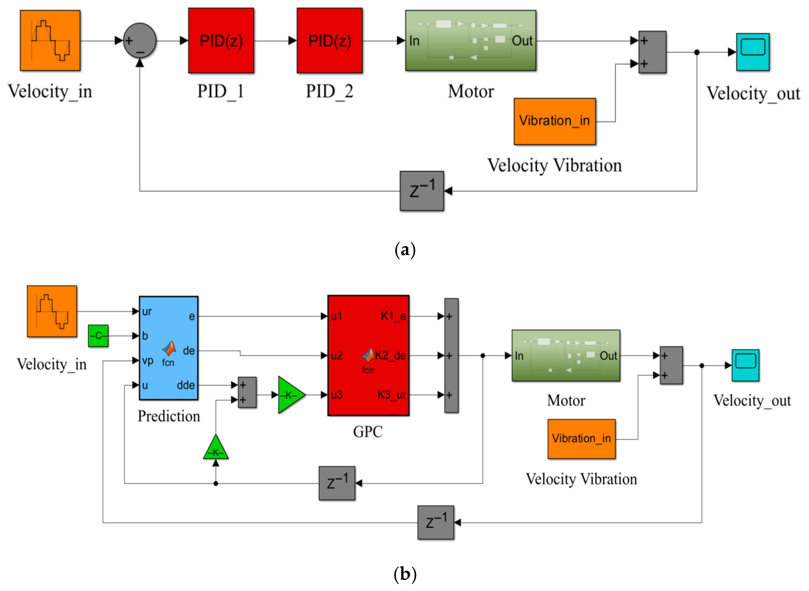
To investigate the performance of the STGPC algorithm, it was compared with the cascade PID control method and the LGPC control method in the MATLAB/Simulink R2023b environment. It should be noted that the LGPC here is based on a continuous-time model and designed using a Taylor expansion as the prediction model. The simulation block diagrams of the three methods are shown in Figure 5.

For comparison, a cascade PID controller is used, with two sets of controller parameters, $K_1^p=0.1803$, $K_1^i=8.4262$, $K_1^d=0$, and $K_2^p=1242.6568$, $K_2^i=255.1134$, $K_2^d=4.6430$. The STGPC parameters are selected as follows: predictive time domain initial value T_p = 0.004, γ = 0.02, observer coefficient ω_b = 300, n = T_p/0.001, where T_p in n is updated iteratively with the control cycle. The time-domain parameters for the LGPC are the same as those for the STGPC.

Under the aforementioned parameter selections, the closed-loop bandwidths of the three simulation systems are similar. Closed-loop characteristics can only reflect part of the system’s features, and the analysis here is provided solely as a reference for parameter selection. Next, we will conduct specific simulation comparison experiments for the three methods.

4.2. Target Experimental Platform

The two-axis, two-frame photoelectric servo turntable shown in Figure 6 was selected as the experimental equipment. The azimuth motor was selected for the experiment, and the vibration interference during operation was collected for simulation. The motor parameters of the turntable are shown in

Table 1. Motor parameters.

Parameter	Value
Lm (H)	0.0053
Rm (Ω)	1.4627
J (kg·m2)	5.0000
Cm (N·m/A)	3.2100
Ce (V/rpm)	0.4500

.

In terms of input, assuming the target’s altitude relative to the turntable is 2000 m, the intercept is 300 m, and the target is moving at a constant speed of 280 km/h, the motion characteristics of the target relative to the turntable can be analyzed as shown in Figure 7. The maximum angular velocity of the target’s motion is 14.85°/s, and the maximum angular acceleration is 2.5°/s². From the maximum angular velocity, the target’s motion can be expressed as a 1.1817° at 2 Hz sinusoidal signal.

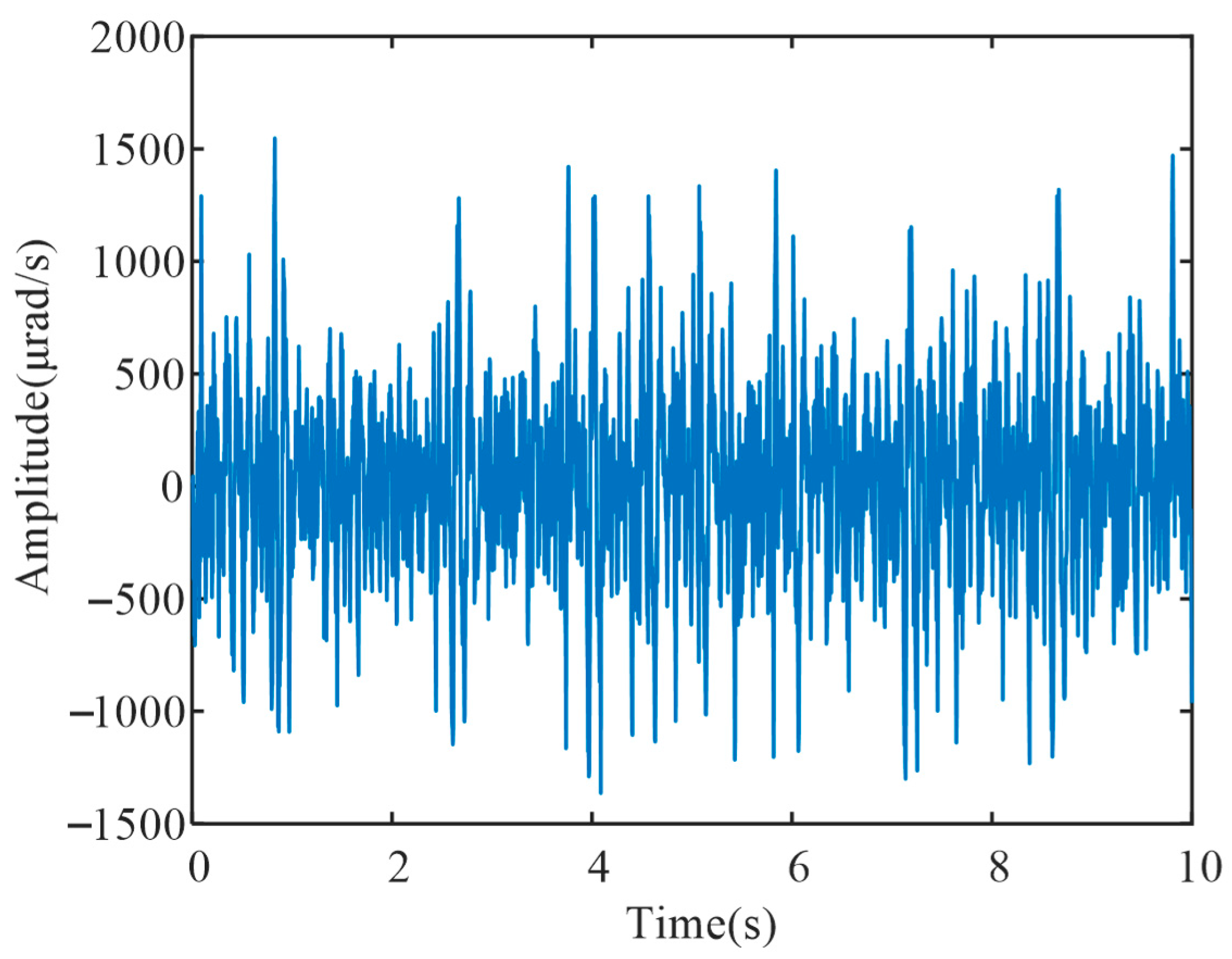
In terms of disturbances, the roll-direction velocity vibrations of the turntable during operation were measured using an inertial navigation system. The vibration data was filtered using a high-pass filter, and a 10 s data segment was extracted for subsequent simulation experiments and analysis. The velocity vibration disturbance is shown in Figure 8. The mean of the disturbance is 11.7875 μrad/s, the standard deviation is 415.3707 μrad/s, and the root mean square (RMS) value is 415.2865 μrad/s, following a Gaussian distribution.

Under the above system inputs and disturbances, the control accuracy, disturbance rejection capability, and parameter self-tuning capability of the STGPC will be compared and verified.

4.3. Tracking Performance Comparison

To demonstrate the superior tracking performance of the STGPC algorithm compared to traditional methods, this section will conduct speed tracking residual comparison experiments between different control algorithms based on the aforementioned simulation setup, parameter selection, and input selection.

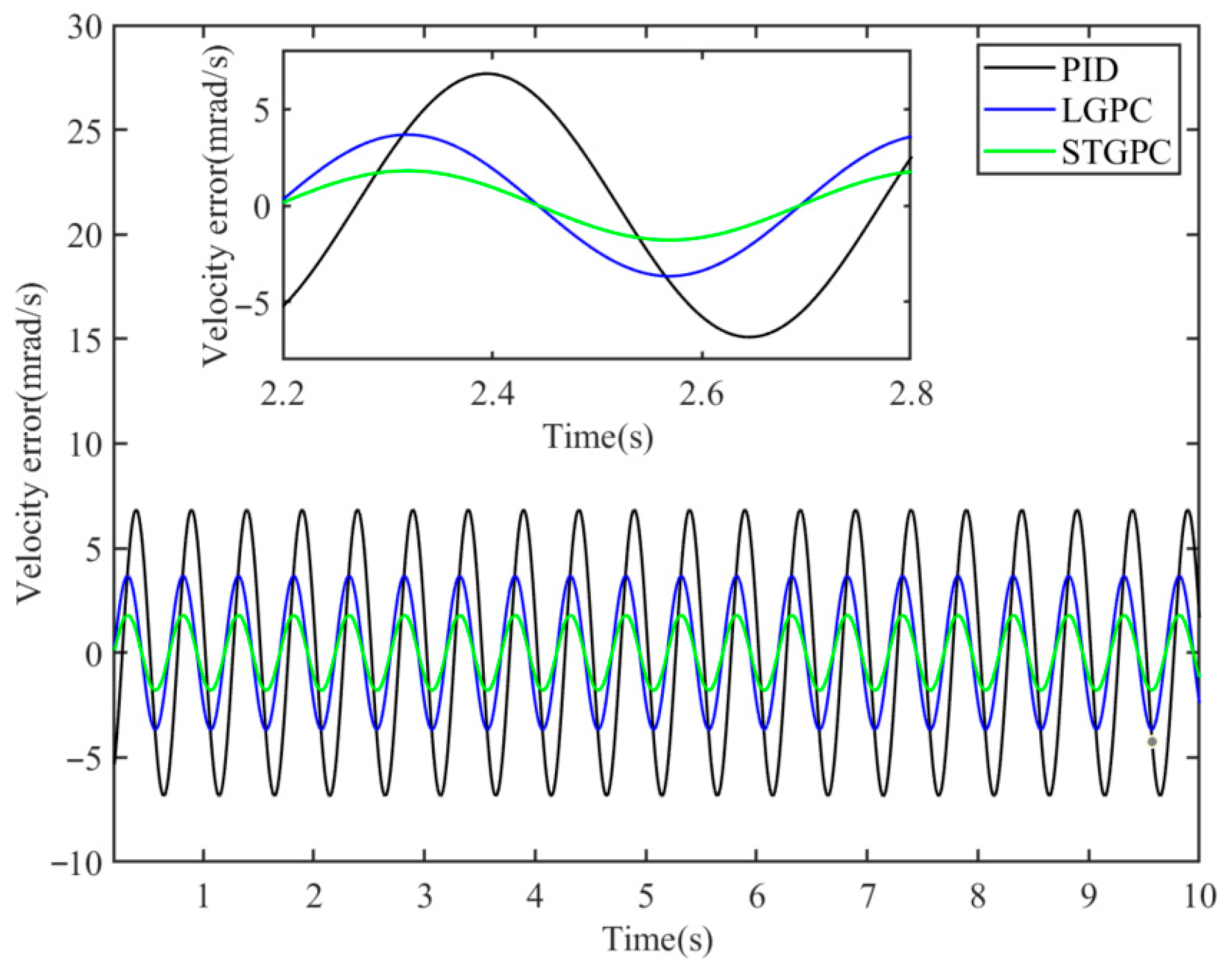
Figure 9 shows a comparison of the speed sine tracking residuals of PID, LGPC, and STGPC. As shown in the figure, LGPC and STGPC have a certain time-domain lead over the traditional PID control, and STGPC has a certain improvement in tracking accuracy compared to the other two methods. The three sets of data in the statistical diagram are calculated separately for their RMS values, and the results are summarized in the tracking residual comparison table shown in

Table 2. Tracking residual comparison table.

Control Method	Velocity Error MAX (mrad/s)	Velocity Error RMS (mrad/s)
PID	6.8409	4.8485
LGPC	3.6751	2.5961
STGPC	1.7992	1.2710

.

As shown in Table 2, STGPC has the smallest speed tracking residual, with the RMS value of the tracking residual reduced by 73.79% compared to PID and by 51.04% compared to LGPC.

4.4. Disturbance Rejection Analysis

4.4.1. Vibration Disturbance Suppression

To verify the algorithm’s ability to suppress vibration interference, this section will introduce speed vibration interference measured in the experimental platform into the system and discuss the suppression levels of different methods.

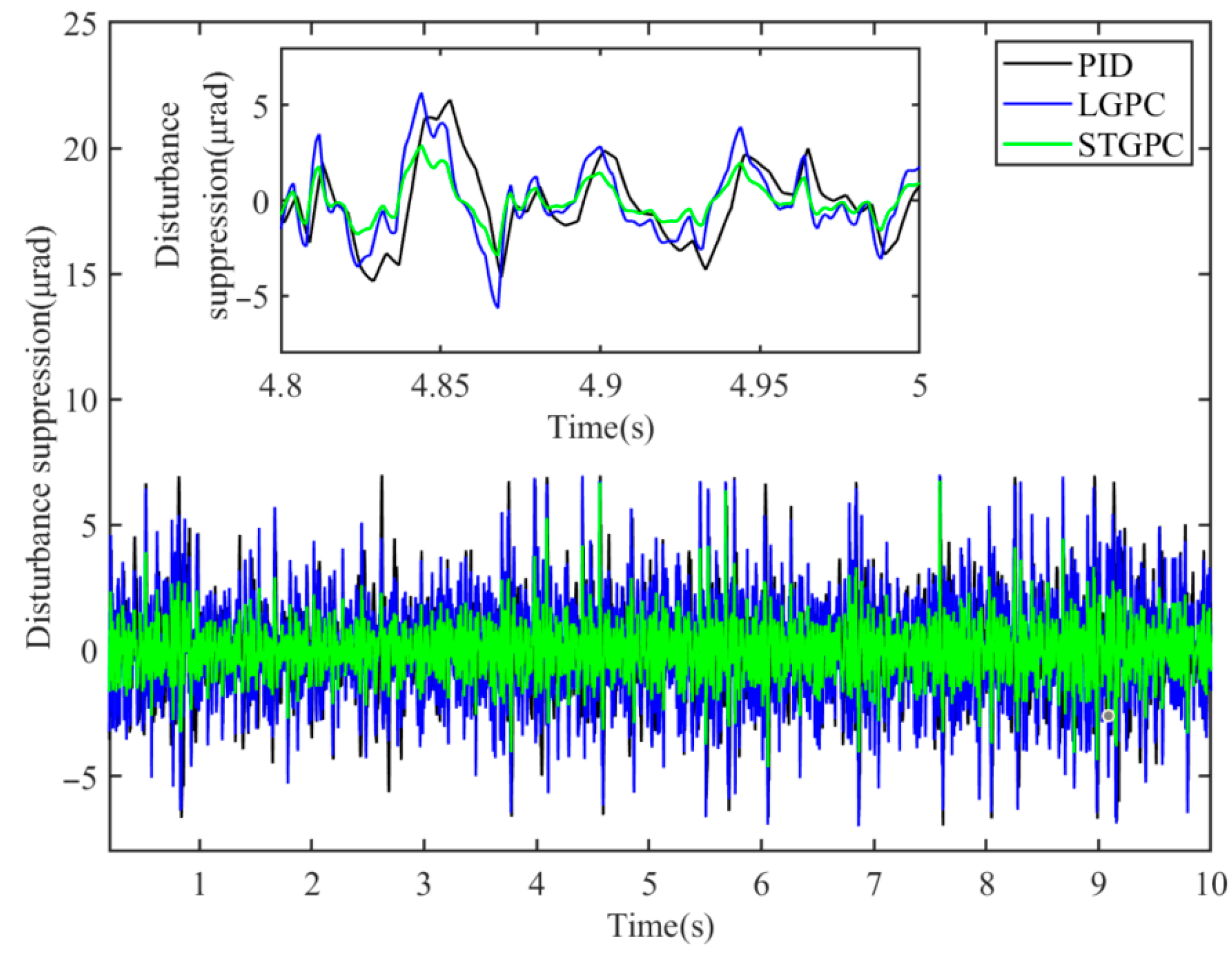
The velocity vibration disturbance shown in Figure 8 is input into the vibration disturbance section of the simulation block diagram in Section 4.1. Tracking residuals are subtracted before and after adding the disturbance using different control methods to obtain the residual change caused by the disturbance, and the resulting curve is plotted as shown in Figure 10.

To specifically compare the disturbance suppression capabilities of several methods, the RMS values were calculated for the extracted data and plotted in a table, as shown in

Table 3. Tracking residual comparison table under vibration interference.

Control Method	Disturbance Suppression RMS (μrad)
PID	2.0198
LGPC	1.9042
STGPC	0.9987

.

As shown in Table 3, the speed loop designed with STGPC has a better ability to suppress disturbances. The suppressed disturbance is 49.45% of PID and 52.45% of LGPC, which is an improvement of 50.55% over PID and 47.55% over LGPC.

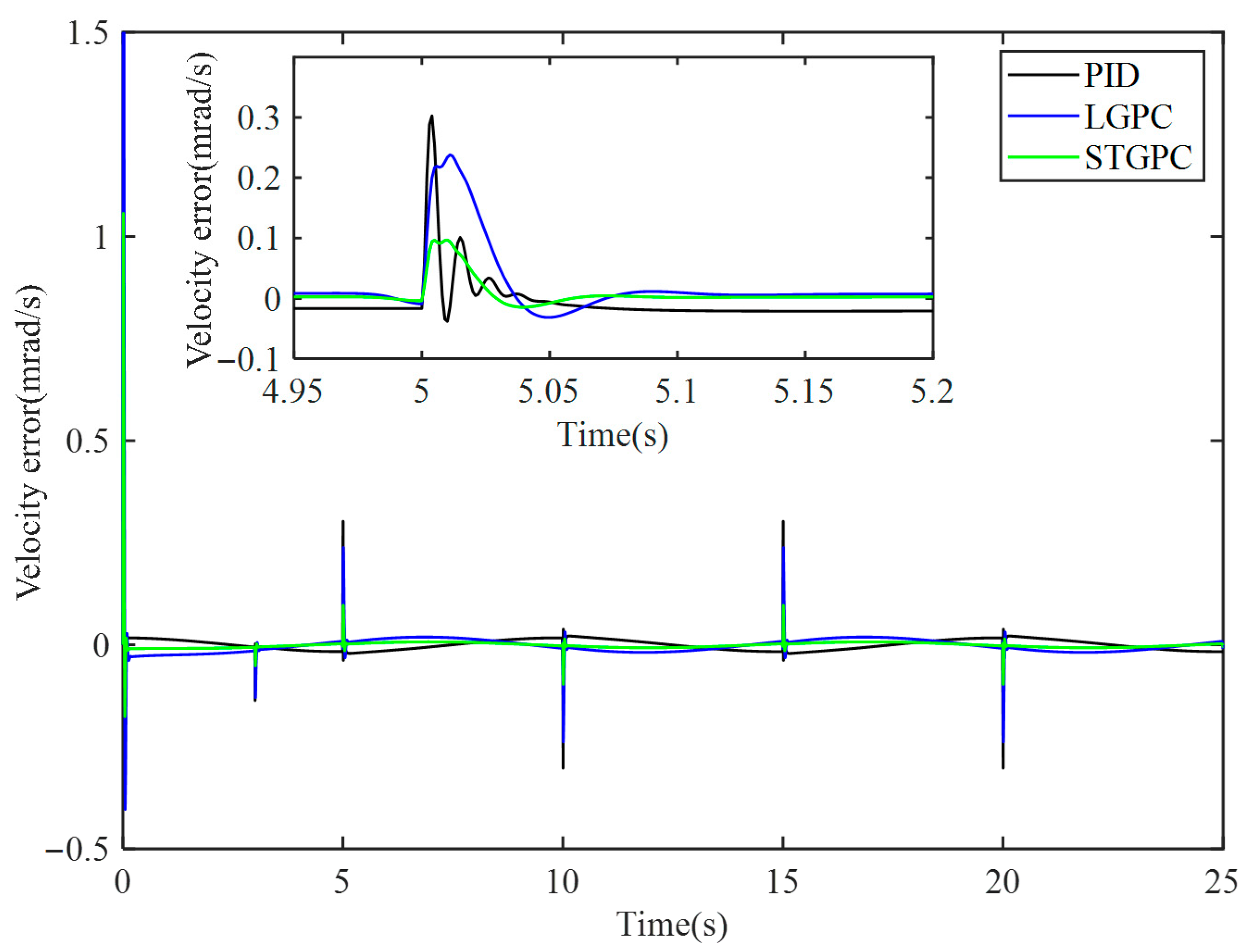
4.4.2. Friction Torque Compensation

During operation, motors are subject to the influence of friction torque, with their dynamic characteristics at low speeds being particularly complex. Specifically, when the driving torque generated by the input current exceeds the maximum static friction torque, the motor begins to accelerate, at which point static friction transitions to Coulomb friction. Since Coulomb friction torque is relatively small, the motor current decreases accordingly, leading to a reduction in speed. When the current decreases to a level insufficient to maintain motion, the motor stops, and the friction mode reverts to static friction. Since the static friction torque is significantly greater than the Coulomb friction torque, the system must increase the current again to restart, thereby forming a periodic “low-speed crawling” phenomenon. Additionally, in the low-speed range, there is a significant nonlinear relationship between the friction torque and rotational speed. Based on the Stribeck friction model, the relationship between motor rotational speed and friction torque can be expressed as Equation (28). Experimental tests conducted using the Elmo driver yielded the friction torque parameters shown in

Table 4. Identified parameter table.

Mc (N·m)	Ms (N·m)	ωs (rpm)	b (N·m/rpm)
2.4596	2.9645	0.1270	0.0196

.

$$M_f=M_c+(M_s-M_c)\cdot e^{\left[-{(\omega /{\omega }_s)}^2\right]}+b\cdot \omega$$

(28)

where M_c is the Coulomb friction torque, M_s is the maximum static friction torque, ω_s is the Stribeck friction torque, b is the viscous friction coefficient; and ω is the angular velocity of the turntable. M_c, M_s, ω_s, and b are the parameters to be identified.

Since the influence of the friction force is particularly significant at low speeds, this section uses a sine wave signal with an amplitude of 14.85° and a frequency of 0.1 Hz as the system simulation input. After integrating the friction model obtained through algorithmic identification into the turntable model, a friction torque disturbance is applied at 3 s. By comparing the speed tracking errors of the three control methods (as shown in Figure 11), the amplitude of speed fluctuations is analyzed to evaluate the compensation capability of different methods against friction torque disturbances. The quantitative comparison results are shown in

Table 5. Table of maximum speed error affected by friction torque.

Control Method	Maximum Speed Error Affected by Friction Torque (mrad/s)
PID	0.3028
LGPC	0.2308
STGPC	0.0968

, where a smaller speed fluctuation amplitude indicates better friction compensation performance of the control method.

As shown in Table 5, the speed loop designed using STGPC exhibits the best compensation effect for friction torque disturbances and is the least affected by friction torque. Compared to PID, STGPC improves friction torque suppression by 68.03%, and compared to LCGPC, STGPC improves friction torque suppression by 59.33%.

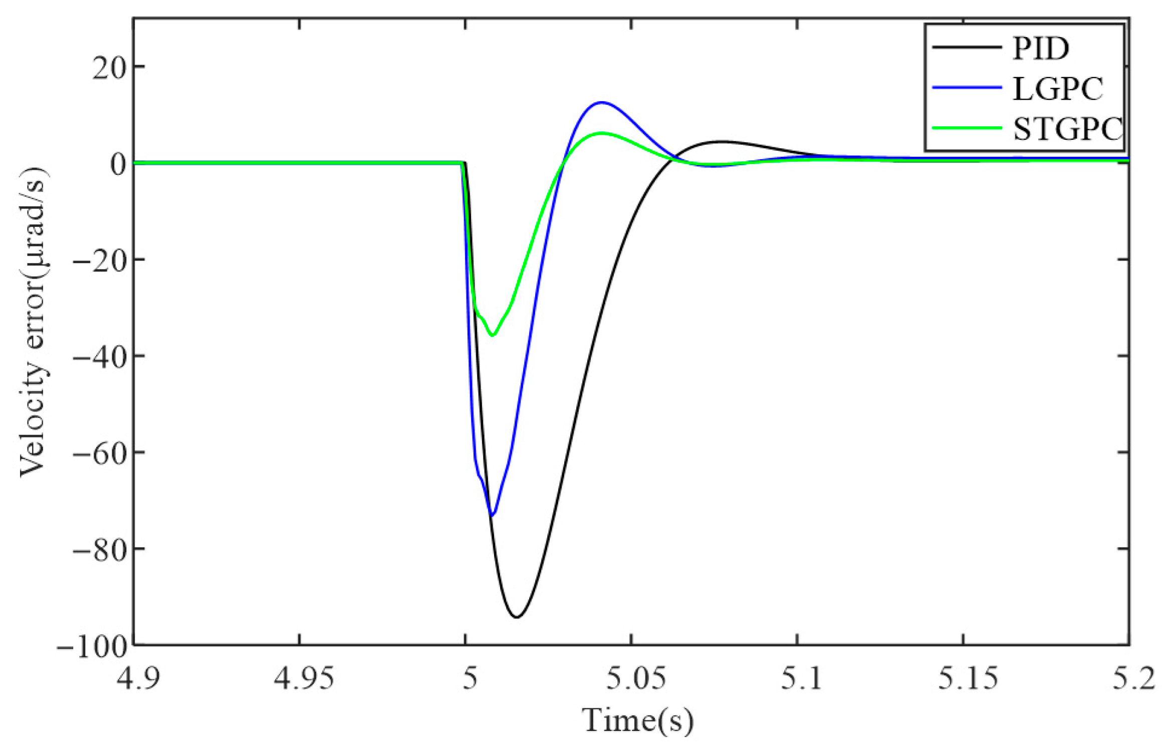
4.4.3. Sudden Load Suppression

In this section, a step signal of approximately 10% of the motor’s peak torque is set to simulate a sudden load. The step starts at 5 s with a magnitude of 6.5 N·m. The suppression capabilities of the three methods against sudden loads are shown in Figure 12, which depicts the control residuals of the system under zero input. Among them, STGPC has better suppression capabilities against sudden loads and faster elimination response to loads.

4.5. Time-Domain Optimization Effectiveness

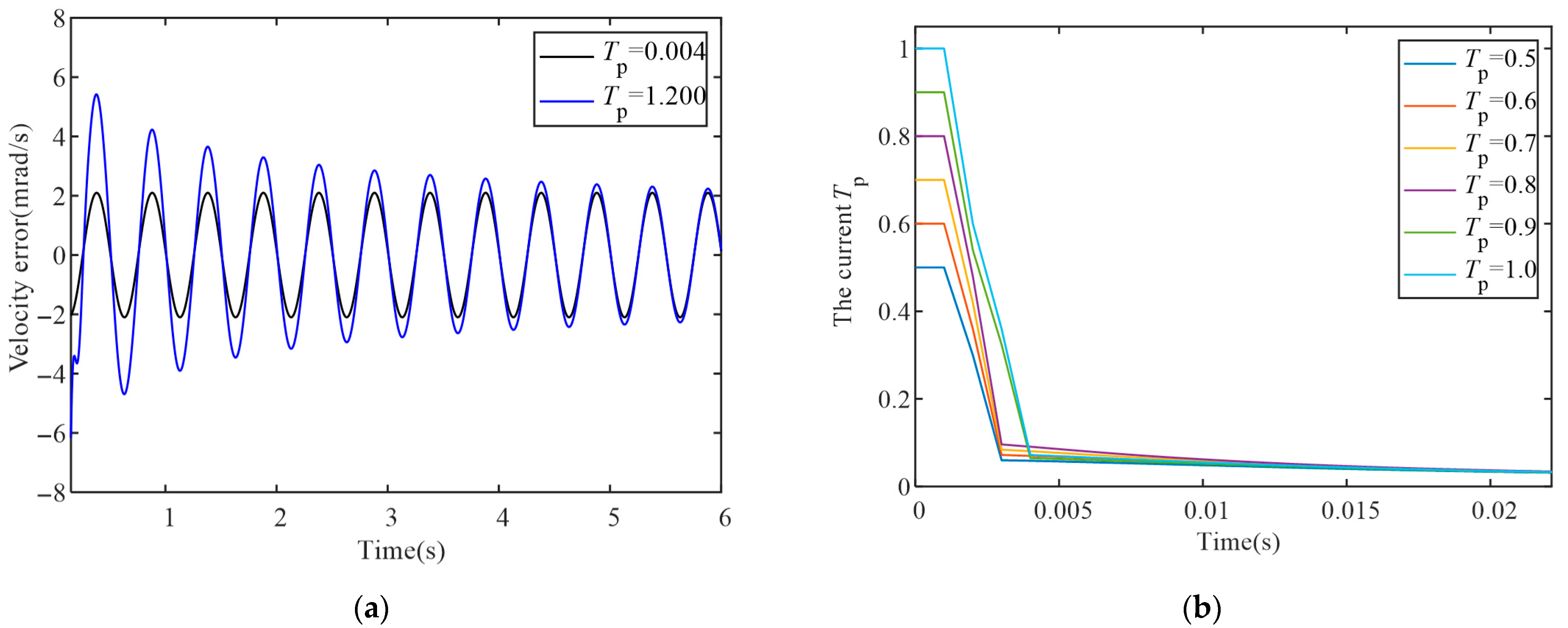
To verify the parameter self-tuning performance based on the gradient descent approach, this section will compare control systems under different time-domain parameters. Through simulation experiments, the system achieved better control performance at T_p = 0.004, while γ = 0 showed no optimization effect. Therefore, one set of parameters for STGPC was set to T_p = 0.004 and γ = 0, serving as the baseline for residual comparison. Another set of parameters was set to T_p = 1.2 and γ = 0.02. The tracking residual plot is shown in Figure 13a. It can be observed that although the red curve was set with an inappropriate T_p value, it can self-adjust under the influence of the time-domain optimization function. The peak of the residuals at around 4 s decreased by 52.60%, gradually approaching better control performance.

To more clearly observe the self-tuning effect of time-domain parameters, multiple sets of different initial T_p values were set. The real-time changes in T_p values are shown in Figure 13b. It can be seen that these T_p values quickly adjust to a reasonable range and then converge slowly. Based on the above analysis, it is inferred that when the controlled object experiences parameter perturbations, the time-domain parameter T_p should be able to self-adjust toward a direction that improves control performance.

To verify this, the gain coefficient K_s is multiplied by the controlled object’s parameters to achieve a ±40% change in the controlled object’s parameters, with K_s set to 0.6, 1.0, and 1.4, respectively, and compare the changes in the system control residual.

As shown in Figure 14, when the controlled object parameter changes to ±40% of the original value, the control system can self-adjust within a certain time frame. After convergence, the control residuals are close, and the control performance remains good, indicating that STGPC has a certain degree of robustness when the model parameter gain is perturbed.

5. Conclusions

The paper addresses the issues of weak disturbance suppression capability and limited accuracy in traditional speed loop control methods for optoelectronic servo turntables, and an improved GPC method with enhanced disturbance rejection capability is proposed. The algorithm employs an extended state observer as the GPC equivalent predictive model to monitor system disturbances and combines gradient descent methods to update predictive time-domain parameters. This method is used for speed loop design, and the control performance of the improved GPC, PID, and LGPC methods is compared. The results demonstrate that compared to the other two methods, the improved GPC reduces speed tracking residuals by 73.79% and 51.04%, respectively, enhances disturbance suppression capability for speed vibration disturbances by 50.55% and 47.55%, respectively, and enhances compensation capability for friction torque disturbances by 68.03% and 59.33%, respectively. Additionally, when the controlled object parameters are perturbed, the predictive time-domain parameters can automatically adjust, exhibiting a certain degree of robustness. These findings underscore not only the robustness but also the superior performance of this advanced algorithm in handling complex control tasks with high precision and efficiency. The next step is to implement and test this algorithm on the turntable platform. The experimental results will be announced later.