Performance Evaluation and Misclassification Distribution Analysis of Pre-Trained Lightweight CNN Models for Hot-Rolled Steel Strip Surface Defect Classification Under Degraded Imaging Conditions

Abstract

Surface defects in hot-rolled steel strip alter the material’s properties and degrade its overall quality. Especially in real production environments, due to time sensitivity, lightweight Convolutional Neural Network models are suitable for inspecting these defects. However, in real-time applications, the acquired images are subjected to various degradations, including noise, motion blur, and non-uniform illumination. The performance of lightweight CNN models on degraded images is crucial, as improved performance on such images reduces the reliance on preprocessing techniques for image enhancement. Thus, this study focuses on analyzing pre-trained lightweight CNN models for surface defect classification in hot-rolled steel strips under degradation conditions. Six state-of-the-art lightweight CNN architectures—MobileNet-V1, MobileNet-V2, MobileNet-V3, NasNetMobile, ShuffleNet V2 and EfficientNet-B0—are evaluated. Performance is assessed using standard classification metrics. The results indicate that MobileNet-V1 is the most effective model among those used in this study. Additionally, a new performance metric is proposed in this study. Using this metric, the misclassification distribution is evaluated for concentration versus homogeneity, thereby facilitating the identification of areas for model improvement. The proposed metric demonstrates that the MobileNet-V1 exhibits good performance under both low and high degradation conditions in terms of misclassification robustness.

1. Introduction

Hot-rolled steel strips play an important role in the national economy and serve as an essential material in various industries, such as automotive, military, machinery manufacturing, and energy sectors. However, unintended surface defects may occur during the manufacturing process. These defects can alter material properties, including corrosion resistance and fatigue strength, ultimately leading to a significant reduction in the quality of the final product [1]. Steel surface inspection is performed to predict defect categories, identify causative factors, and provide important information for corrective actions, while traditionally, human experts manually assess the surface quality of steel strips; this method is highly subjective, labor-intensive, and inefficient for real-time inspection tasks [2,3]. Thus, the development of a new inspection method is essential to replace traditional approaches.

Recently, deep learning techniques, especially Convolutional Neural Networks (CNNs), have been used for the detection and classification of steel surface defects. Khanam et al. [4] demonstrated the practical applications of CNN models across industries. Wen et al. [5] presented a comprehensive study of recognition algorithms, including CNN-based approaches. Yi et al. [6] proposed a system that includes a preprocessing step; the processed images were fed to a novel CNN. Zhu et al. [7] designed a lightweight model using ShuffleNet V2, while Mao and Gong [8] employed a MobileNet-V3 module. Liu et al. [9] surveyed deep and lightweight CNN architectures for industrial scenarios. Bouguettaya and Zarzour [10] conducted a comparative study on different pre-trained CNN models and proposed a custom classifier. Wi et al. [11] developed a cost-efficient segmentation labeling framework that combines label enhancement and deep-learning-based anomaly detection in industrial applications. Ashrafi et al. [12] proposed various deep learning-based vision approaches, including both semantic segmentation and object detection. Ibrahim and Tapamo [13] integrated VGG16 components into a new CNN for industrial quality inspection. Jeong et al. [14] presented Hybrid-DC, a hybrid CNN–Transformer architecture for real-time quality control in high-precision manufacturing.

In real production environments, images acquired by image acquisition equipment often suffer from various types of noise, motion blur, and non-uniform illumination, which significantly degrade the performance of surface defect inspection methods. Therefore, once acquired, an image typically undergoes preprocessing (e.g., enhancement) before being input to a CNN. This approach effectively improves the perceptibility and enhances the image characteristics to meet the requirements of subsequent analysis (i.e., defect detection and defect classification) [9,15,16]. In the literature, various preprocessing techniques have been employed to enhance image quality, such as histogram equalization [17], Gaussian filtering [18], Sobel and Prewitt operators [19], and CNN [20], among others. However, a single filter may not only smooth the image but also obscure important details. To address this issue, researchers have attempted to combine multiple filters to suppress noise [16]. However, this approach increases processing time, and image enhancement should be efficient in terms of time and resources, as it serves as a preprocessing step for the defect classification task [16].

Studies in the literature for steel surface defect inspection have been conducted on both deep and lightweight CNN models. In this work, lightweight CNN models are analyzed. Since lightweight CNN models have fewer parameters and lower computational cost, they can run faster on a system and minimize latency, making them particularly suitable for time-sensitive real-time applications. As noted earlier, images acquired in real-world production settings are often degraded by noise, motion blur, and non-uniform illumination. In the literature, model performance has typically been evaluated either on original images alone or on a mixture of original and degraded images. In this study, only degraded images are used for testing, since real-world inspection must tolerate degraded inputs with low latency; accordingly, robustness to degradation is the primary focus. This is particularly important for lightweight CNN models operating in real-time systems, as the time required for image enhancement preprocessing, which is especially needed for degraded images, is more critical for time-sensitive real-time applications. The better lightweight CNN models perform on degraded images, the less need there will be for preprocessing techniques aimed at image enhancement. Thus, this study aims to assist industries and researchers by analyzing lightweight CNN models for surface defect recognition in terms of time and performance on degraded images that have not undergone any preprocessing.

The publicly available Northeastern University (NEU-CLS) dataset [1] is used for steel surface defect images in this study. Original images are used for training and validation, whereas degraded images are used for testing without any preprocessing. Six pre-trained lightweight CNN models are analyzed. The base of each CNN is kept frozen and only the classifier is trained. Both accuracy-related metrics and normalized inference time are reported to assess model performance.

In the literature, models tested using original images generally exhibit a low misclassification rate, and these misclassifications tend to be concentrated in a specific class. This situation allows for a clearer analysis of the relationship between misclassified classes. However, models tested with degraded images are expected to have a higher error rate as an anticipated outcome. Thus, it increases the likelihood that misclassified instances are distributed across multiple classes rather than being concentrated in a single class, which makes the analysis of the relationship between misclassified classes more challenging. In this study, a new performance metric is proposed to analyze the distribution of misclassifications: Adjusted False Classification Index (AFCI). AFCI is designed to assess how homogeneously misclassifications are distributed. Unlike other misclassification-analysis techniques, AFCI quantifies class-wise error dispersion via the Gini coefficient (GC) and conditions the analysis on the False Negative Rate (FNR). It therefore takes into account both the error’s proportion and the homogeneity of their distribution across other predicted classes (i.e., clustered vs. homogeneous). By analyzing the distribution of misclassifications through this index, the improvement needs of the model can be identified.

2. Materials and Methods

In this study, a performance evaluation of pre-trained lightweight CNN models for hot-rolled steel strip surface defect classification under degraded imaging conditions is performed. Then, a performance metric to analyze the distribution of misclassifications is proposed.

2.1. Degraded Imaging Conditions

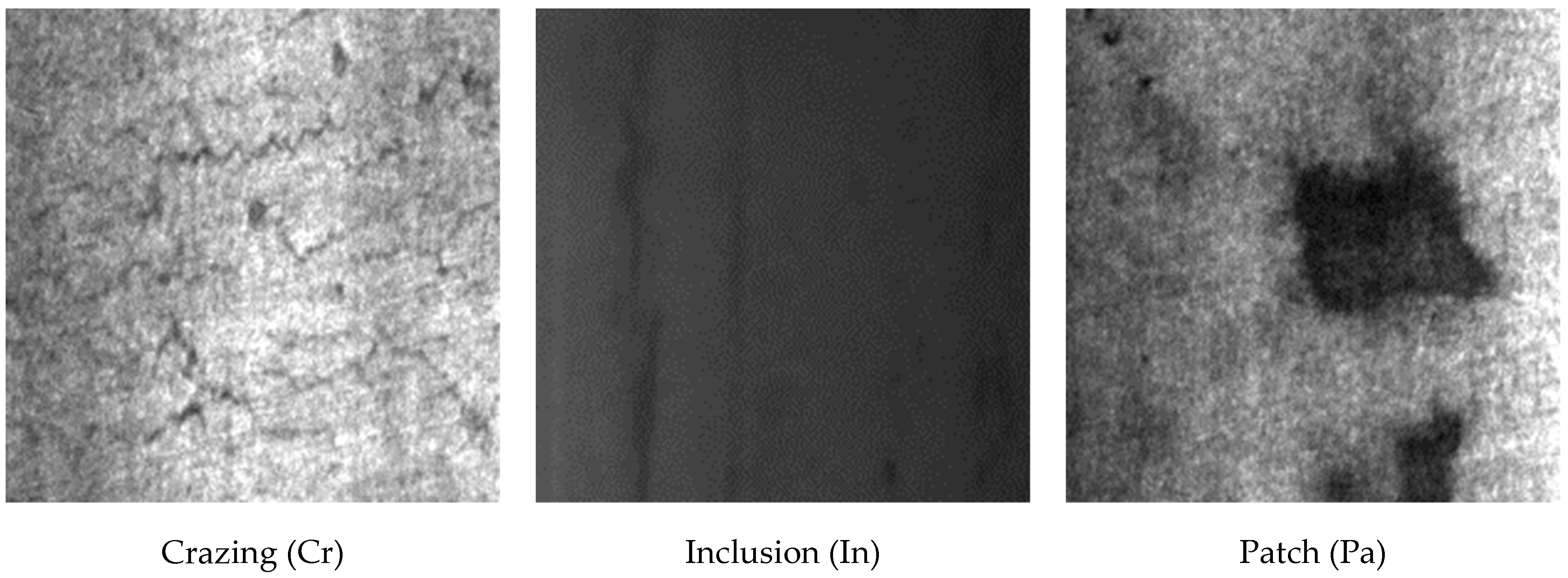
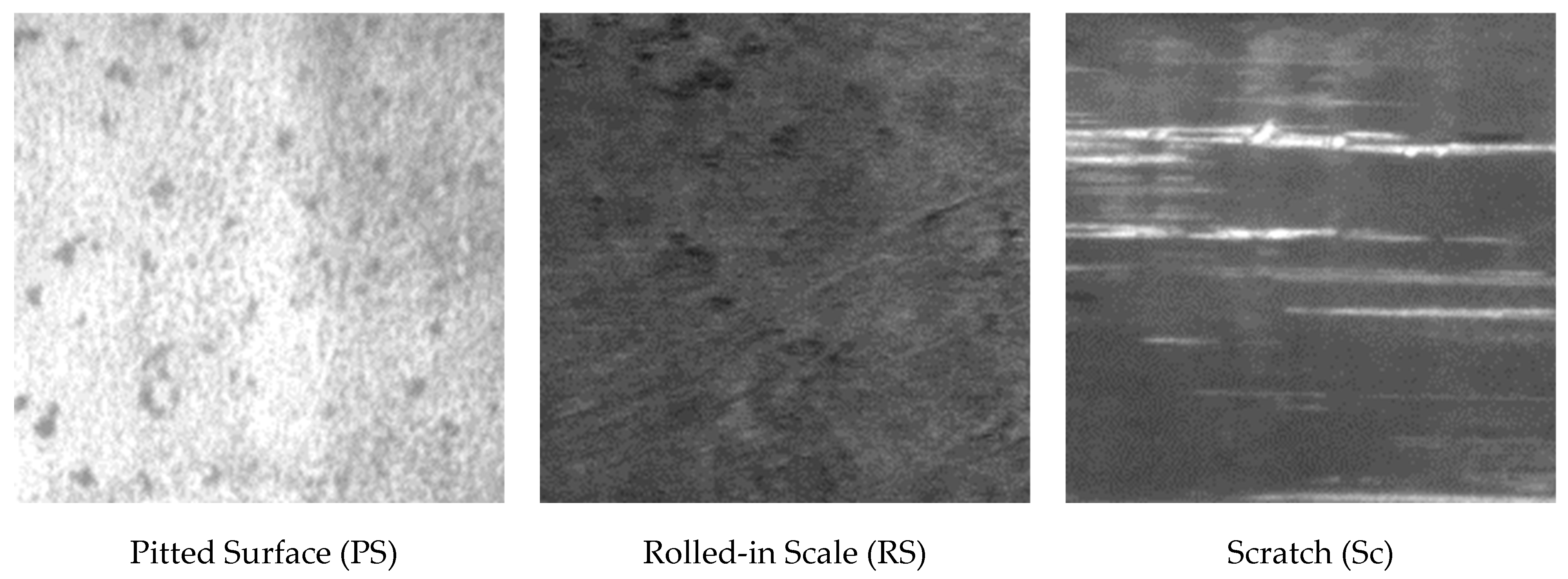
In the literature, the NEU-CLS dataset is frequently used to demonstrate the effectiveness of CNN models for surface defect recognition. The NEU-CLS dataset comprises six common hot-rolled steel strip defects: Crazing (Cr), Inclusion (In), Pitted Surface (PS), Patch (Pa), Rolled-in Scale (RS), and Scratch (Sc). It includes a total of 1800 images, with 300 images per defect category. Each image has a resolution of 200 × 200 pixels. NEU-CLS images are used for training, validation and test sets in this study. Figure 1 presents sample images from each category in the NEU-CLS dataset. These images are original and not degraded.

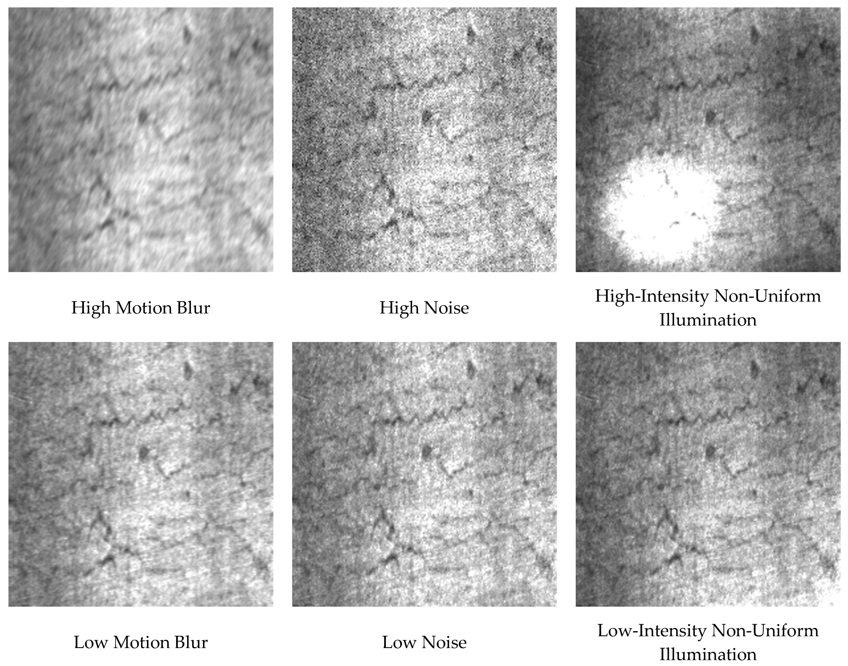
I use 1440 original images for training, 180 original images for validation, and 180 degraded images (noise, motion blur, or non-uniform illumination) for testing. During steel image acquisition, noise arises, and, in particular, Gaussian noise is a type of sensor noise that negatively impacts subsequent procedures [21]. Similarly to [1,2], Gaussian noise is added to each defect sample in the test set with two signal-to-noise ratio (SNR) levels: 50 dB (low noise) and 20 dB (high noise). For each noise level, 180 noisy images are generated. Due to the rolling speed, the captured defect images typically exhibit noticeable motion blur effects [1,2]. The blurred image is generated by convolving the original image with a motion filter that approximates the camera trajectory. I set the camera motion length (L_cm) to 2 and 5, as in [2], where L_cm = 2 results in a low motion blur effect, while L_cm = 5 produces a higher motion blur effect. For each motion length, I generate 180 motion-blurred images using random motion angles between 0° and 360°. Since it is challenging to set up light sources that provide perfect illumination for making defects visible during the image acquisition process, evaluating the performance of defect classifiers under various illumination conditions is crucial [2]. To simulate images with different non-uniform illumination effects, I use a third-order polynomial model to generate slow-varying intensity bias fields [22], which are then combined with the original images. I set the luminance range (α) of the bias fields to ±0.4 and ±1, as in [2], where α = ±0.4 yields low-intensity non-uniform illumination, whereas α = ±1 yields high-intensity non-uniform illumination. For each non-uniform illumination condition, 180 images are acquired to evaluate classification performance. Figure 2 presents a subset of degraded versions of the Crazing image, which is originally depicted in Figure 1.

Using a test set comprising mildly and highly degraded images, performance under degraded imaging conditions is evaluated across multiple metrics.

2.2. Model Training

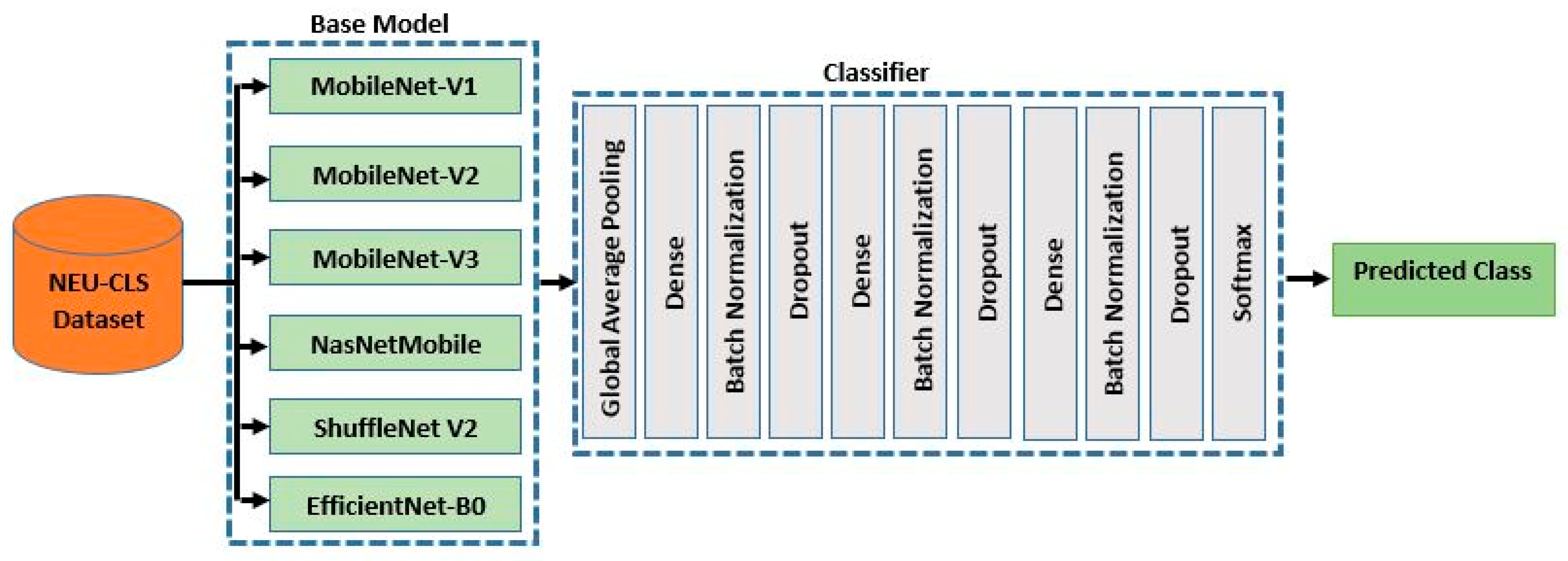
Training a model from scratch is often challenging as it requires a large number of training examples [23]. Due to the low occurrence probability of steel surface defects, constructing a large-scale defect dataset for training a CNN model from scratch is both difficult and time-consuming. Consequently, utilizing a pre-trained model as the basis for classifier development is recommended [2,23]. This technique, known as transfer learning, leverages knowledge acquired from previous tasks to enhance performance on a new task; for example, it involves utilizing feature parameters learned from the ImageNet classification task to improve surface defect classification [10,23]. Accordingly, in this study, the base of the pre-trained CNN is kept frozen, and only the classifier is trained. Six state-of-the-art lightweight CNN architectures are employed—MobileNet-V1 [24], MobileNet-V2 [25], MobileNet-V3 [26], NasNetMobile [27], ShuffleNet V2 [28] and EfficientNet-B0 [29]. In each case, the base model is utilized as the feature extraction component, while the classifier part is replaced with the proposed classifier from [10], which demonstrated successful performance. Figure 3 shows the architecture of the classification model used in this study.

Experiments are implemented in Python 3.9.13. Training is conducted for 50 epochs using Adam (LR = 1 × 10⁻⁴). The loss function employed is categorical cross-entropy, and a batch size of 16 is used. I ensure reproducibility by fixing the train/validation/test splits and holding all hyperparameters constant. Randomness inherently occurs during training. To mitigate its effects, I control the sources of randomness by stabilizing them throughout the training process. Additionally, for each architecture, results are averaged over ten runs (frozen base; trainable classifier). Therefore, the results are generally fractional, and the term ‘averaged’ is not explicitly stated for each result.

2.3. Evaluation Metrics

In deep learning-based solutions, the performance of the model is assessed using evaluation metrics. This study employs several evaluation metrics to compare the performance of pre-trained lightweight CNN models: accuracy, accuracy standard deviation, inference time, recall, precision, F1-score, and the confusion matrix.

2.3.1. Accuracy

Accuracy is a fundamental evaluation metric in classification tasks, quantifying the proportion of correctly classified instances relative to the total number of instances. It is widely utilized to assess the overall performance of a model. Accuracy is defined as in Equation (1):

Accuracy = (TP + TN)/(TP + TN + FP + FN)

(1)

where

• TP (True Positives): Instances that are correctly predicted as positive.
• TN (True Negatives): Instances that are correctly predicted as negative.
• FP (False Positives): Instances that are incorrectly predicted as positive when they are actually negative.
• FN (False Negatives): Instances that are incorrectly predicted as negative when they are actually positive.

2.3.2. Accuracy Standard Deviation

Accuracy standard deviation (ASD) quantifies the consistency of a model’s performance across different types of degradation. A lower ASD indicates that the model exhibits more stable performance.

2.3.3. Precision, Recall, and F1-Score

Precision is the proportion of predicted positives that are true positives; recall is the proportion of actual positives that are correctly identified. F1-score combines precision and recall into a single value, providing a balance between the two metrics. The formulas of precision, recall and F1-score are given in Equations (2)–(4), respectively.

Precision = TP/(TP + FP)

(2)

Recall = TP/(TP + FN)

(3)

F1-score = 2 × (Precision × Recall)/(Precision + Recall)

(4)

2.3.4. Confusion Matrix

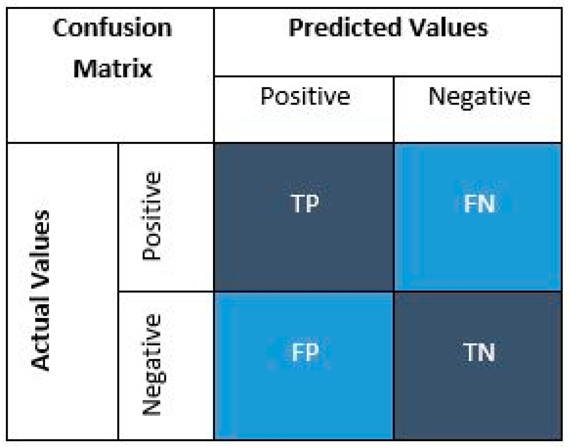
A confusion matrix represents the performance of a classification model by summarizing the counts of actual and predicted classifications across different classes. Figure 4 illustrates a binary classification confusion matrix. The vertical axis represents the actual labels, while the horizontal axis represents the predicted labels. TP and TN indicate correct predictions made by the model, whereas FP and FN represent incorrect predictions.

2.3.5. Inference Time

Inference time refers to the duration a model takes to process an input and produce an output. It is a critical metric for assessing the efficiency of a deep learning model, especially in real-time applications, where rapid decision-making is essential.

In this study, the inference time for each model is calculated. For each model, the inference time is measured ten times for a single image, and the average of these measurements is taken as the final inference time. However, because inference time is platform-dependent, I report a normalized inference time scaled to the slowest model: each value is divided by the largest time observed across models (“1” denotes the slowest; smaller is better). This normalization allows us to use the “normalized inference time” values for a fair comparison of model performance.

2.4. Proposed Performance Metric

There are various metrics to compare model performance, each providing a different perspective on the analysis of the confusion matrix. In this study, a novel performance metric called the Adaptive False Classification Index (AFCI) is proposed. AFCI is designed to analyze the distribution of misclassifications and consists of two key parameters: GC and FNR.

This study uses the GC to measure the imbalance in the distribution of misclassifications. The GC is defined as in Equation (5):

$$\mathrm{G}\mathrm{C}=1-\sum _{i=1}^n{P}_i^2$$

(5)

where $n$ is the number of misclassified classes, and the misclassification proportion $P_i$ for class $i$ is the ratio of the number of instances misclassified in class $i$ to the total number of misclassified instances. The maximum attainable value of the GC (denoted GC_M) depends on $n$ and is given by:

$${\mathrm{G}\mathrm{C}}_{\mathrm{M}}=1-{\displaystyle \frac{1}{n}}$$

(6)

In my experiments ($n$= 5), GC_M = 0.8. To assess the distribution of misclassifications, I use the normalized Gini coefficient (GC_N), as defined in Equation (7):

$${\mathrm{G}\mathrm{C}}_{\mathrm{N}}={\displaystyle \frac{\mathrm{G}\mathrm{C}}{{\mathrm{G}\mathrm{C}}_{\mathrm{M}}}}$$

(7)

GC_N is normalized to [0, 1]; see Equation (7). The FNR, another key parameter for measuring the imbalance in the distribution of misclassifications, is defined by the following equation.

$$\mathrm{F}\mathrm{N}\mathrm{R}={\displaystyle \frac{\mathrm{F}\mathrm{N}}{\mathrm{T}\mathrm{P}+\mathrm{F}\mathrm{N}}}$$

(8)

In this study, the FNR parameter is used to indicate that for very small FNR values, the imbalance in the distribution of misclassifications is not taken into account. Consequently, the proposed index is represented by the following equation:

$$\mathrm{A}\mathrm{F}\mathrm{C}\mathrm{I}=\left\{\begin{array}{cc}\varnothing ,\hfill & \hfill \mathrm{FNR}<1-e^{-w}\\ {\mathrm{G}\mathrm{C}}_{\mathrm{N},}\hfill & \hfill otherwise\end{array}\right.$$

(9)

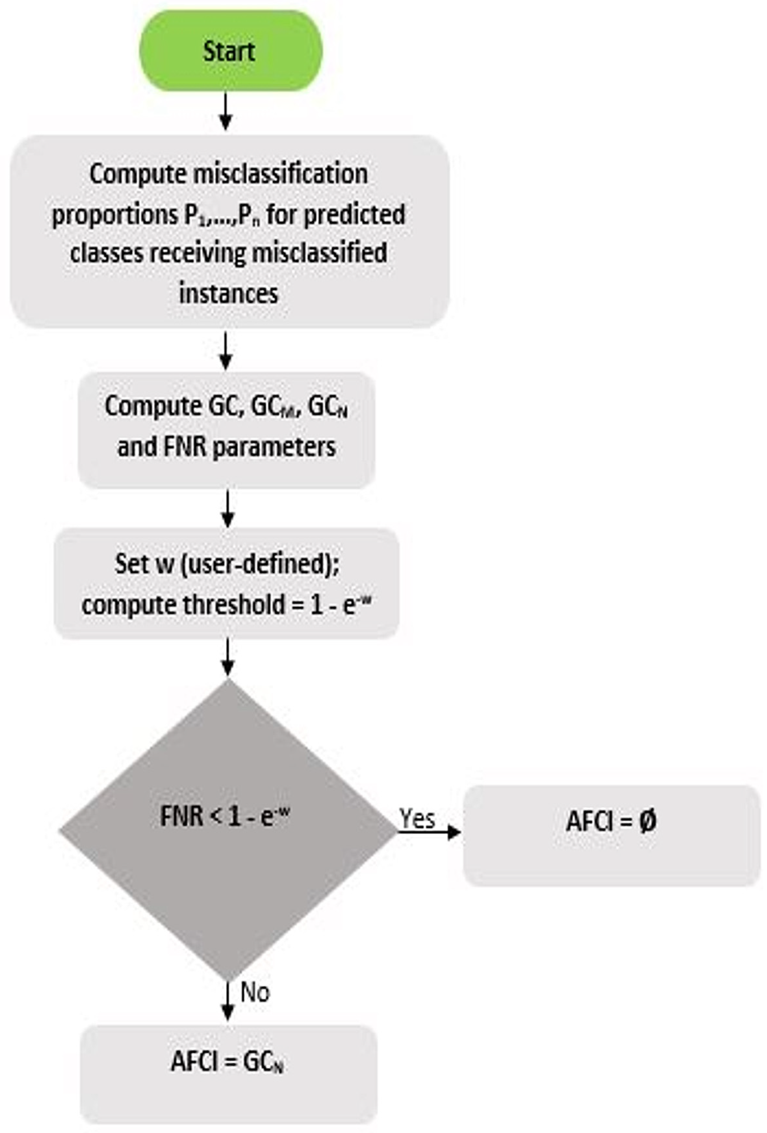
where $w$(weighting parameter) is the impact of FNR on AFCI. The per-class AFCI computation workflow is shown in Figure 5.

As shown in Figure 5, if the FNR $<1-e^{-w}$, the AFCI is considered null (∅), i.e., the misclassification distribution is ignored. Otherwise, it is equal to the GC_N, meaning that the AFCI has a defined value. An AFCI value of 0 indicates that all misclassified instances are concentrated in a single misclassified class, representing maximum imbalance. Conversely, an AFCI value of 1 indicates that the misclassified instances are uniformly distributed among the misclassified classes, reflecting a homogeneous distribution. Thus, the AFCI serves as a metric for evaluating the misclassification distribution, taking into account FNR. By using this index, the concentration versus homogeneity of the misclassification distribution can be analyzed, allowing identification of areas where the model requires improvement.

3. Results and Discussion

To evaluate the performance of the aforementioned pre-trained lightweight CNN models, I first employ the accuracy and normalized inference time evaluation metrics for all degraded conditions, as shown in

Table 1. Accuracy table.

Degraded Condition	Pre-Trained Lightweight CNN Models
	MobileNet-V3	MobileNet-V2	MobileNet-V1	NasNetMobile	ShuffleNet V2	EfficientNet-B0
Low-Intensity Non-Uniform Illumination	0.9152	0.9937	0.9987	0.9907	0.9532	0.7232
High-Intensity Non-Uniform Illumination	0.8815	0.9457	0.9789	0.9541	0.9207	0.7287
High Noise	0.8106	0.9548	0.9646	0.9744	0.7652	0.7235
Low Noise	0.9146	0.9957	0.9993	0.9956	0.9561	0.7422
Low Motion Blur	0.8722	0.9948	0.9972	0.9941	0.9144	0.7232
High Motion Blur	0.7817	0.9115	0.9602	0.9530	0.8085	0.7250

and

Table 2. Normalized Inference Time.

Metric	Pre-Trained Lightweight CNN Models
	MobileNet-V3	MobileNet-V2	MobileNet-V1	NasNetMobile	ShuffleNet V2	EfficientNet-B0
Normalized Inference Time	0.6694	0.7904	0.7637	0.9550	0.6482	1

, respectively.

Among all models, based on Table 1 and Table 2, EfficientNet-B0 exhibits the lowest accuracy and the highest normalized inference time; therefore, it is excluded from further analysis. In general, MobileNet-V1 achieves the best results. Only under high noise conditions, NasNetMobile outperforms MobileNet-V1. When comparing the normalized inference times of these two models, MobileNet-V1 completes the operation in a significantly shorter time. Although MobileNet-V1 and MobileNet-V2 have approximately the same normalized inference times, MobileNet-V1 achieves significantly better results, particularly under high-intensity non-uniform illumination and high motion blur conditions. Among the models, MobileNet-V3 and ShuffleNet V2 have significantly shorter normalized inference times. As shown in Table 1, ShuffleNet V2 achieves better results than MobileNet-V3 for all degradations except high noise. Although ShuffleNet V2 has a better normalized inference time than MobileNet-V2, MobileNet-V1, and NasNetMobile, it performs worse than these models across all types of degradations. In this study, the ASD is computed for each model across the six degradation conditions. The resulting ASDs for MobileNet-V3, MobileNet-V2, MobileNet-V1, NasNetMobile, and ShuffleNet V2 are 0.0551, 0.0346, 0.0178, 0.0197, and 0.0801, respectively. Among these models, MobileNet-V1 has the lowest ASD, indicating that it exhibits the most consistent performance across different types of degradation. As a result, if inference time is the only priority, ShuffleNet V2 can be preferred. However, when accuracy, ASD, and normalized inference time are evaluated together, MobileNet-V1 emerges as the best option among the models used in this study.

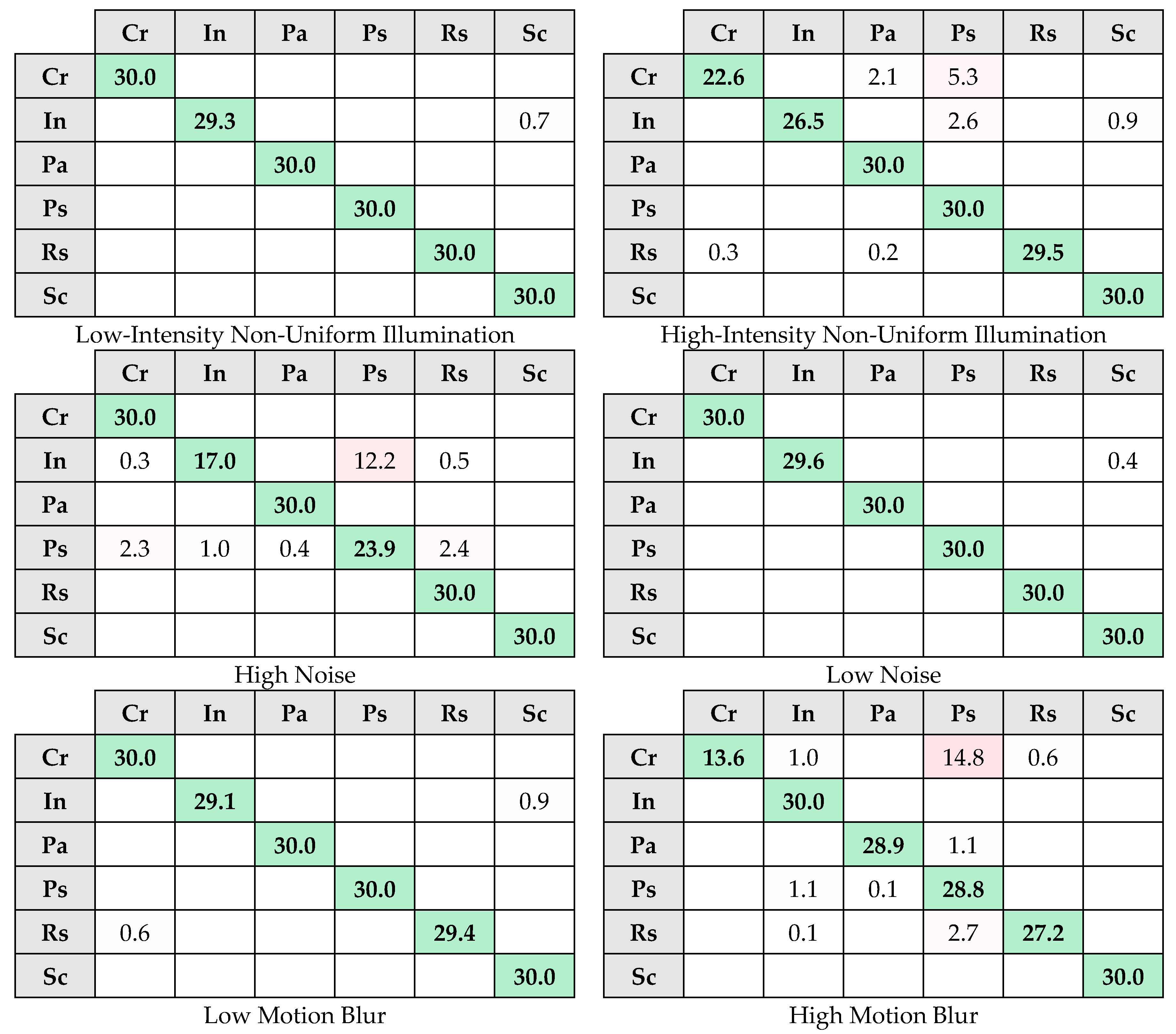
The classification performances of MobileNet-V1 and ShuffleNet V2 are presented in

Table 3. The classification performance of MobileNet-V1.

Degraded Condition	Defect Class	Precision	Recall	F1-Score
Low-Intensity Non-Uniform Illumination	Cr	1	1	1
	In	1	0.9767	0.9882
	Pa	1	1	1
	Ps	1	1	1
	Rs	1	1	1
	Sc	0.9772	1	0.9885
High-Intensity Non-Uniform Illumination	Cr	0.9869	0.7533	0.8544
	In	1	0.8833	0.9381
	Pa	0.9288	1	0.9631
	Ps	0.7916	1	0.8837
	Rs	1	0.9833	0.9916
	Sc	0.9709	1	0.9852
High Noise	Cr	0.9203	1	0.9585
	In	0.9444	0.5667	0.7083
	Pa	0.9868	1	0.9934
	Ps	0.6621	0.7967	0.7232
	Rs	0.9119	1	0.9539
	Sc	1	1	1
Low Noise	Cr	1	1	1
	In	1	0.9867	0.9933
	Pa	1	1	1
	Ps	1	1	1
	Rs	1	1	1
	Sc	0.9868	1	0.9934
Low Motion Blur	Cr	0.9804	1	0.9901
	In	1	0.9700	0.9848
	Pa	1	1	1
	Ps	1	1	1
	Rs	1	0.9800	0.9899
	Sc	0.9709	1	0.9852
High Motion Blur	Cr	1	0.4533	0.6239
	In	0.9317	1	0.9646
	Pa	0.9966	0.9633	0.9797
	Ps	0.6076	0.9600	0.7442
	Rs	0.9784	0.9067	0.9412
	Sc	1	1	1

and

Table 4. The classification performance of ShuffleNet V2.

Degraded Condition	Defect Class	Precision	Recall	F1-Score
Low-Intensity Non-Uniform Illumination	Cr	0.9167	0.9900	0.9519
	In	0.6424	0.9400	0.7632
	Pa	0.9125	0.9733	0.9419
	Ps	0.9037	0.5633	0.6941
	Rs	0.9927	0.9100	0.9496
	Sc	0.9177	0.7800	0.8432
High-Intensity Non-Uniform Illumination	Cr	0.8087	0.7467	0.7764
	In	0.6484	0.7500	0.6955
	Pa	0.7933	0.9467	0.8632
	Ps	0.5733	0.6000	0.5863
	Rs	0.9747	0.7700	0.8603
	Sc	0.8539	0.7600	0.8042
High Noise	Cr	0.2037	1	0.3384
	In	0	0	0
	Pa	0.7134	0.7633	0.7375
	Ps	1	0.0033	0.0067
	Rs	0	0	0
	Sc	1	0.0067	0.0133
Low Noise	Cr	0.8596	1	0.9245
	In	0.6907	0.9600	0.8034
	Pa	0.9245	0.9800	0.9515
	Ps	0.9343	0.6167	0.7430
	Rs	1	0.8533	0.9209
	Sc	0.9160	0.8000	0.8541
Low Motion Blur	Cr	1	0.5767	0.7315
	In	0.5365	0.9567	0.6874
	Pa	0.8502	0.9267	0.8868
	Ps	0.7591	0.5567	0.6423
	Rs	0.7725	0.6000	0.6754
	Sc	0.8109	0.8433	0.8268
High Motion Blur	Cr	0.9167	0.0367	0.0705
	In	0.3638	0.9700	0.5291
	Pa	0.9546	0.2100	0.3443
	Ps	0.3813	0.5300	0.4435
	Rs	0.3750	0.0400	0.0723
	Sc	0.4863	0.7667	0.5951

, respectively. The confusion matrices of MobileNet-V1 and ShuffleNet V2 are shown in Figure 6 and Figure 7, respectively.

Consistent with Figure 4, each confusion matrix in Figure 6 and Figure 7 follows the same axis representation, with the horizontal axis for predicted labels and the vertical axis for actual labels. To reduce visual clutter, zero-valued off-diagonal cells are left blank in the confusion matrices in Figure 6 and Figure 7; diagonal values are always displayed. That is, empty cells in Figure 6 and Figure 7 indicate zero values. As observed in Table 1, MobileNet-V1 demonstrates a high accuracy rate under low-level degradations. According to Table 3, when examining the F1-score for MobileNet-V1 under all three types of low-level degradation, only the Inclusion and Scratch classes remain below 100% performance across all low-level degradation levels. For all three types of low-level degradation, the recall value for the Inclusion class remains low, indicating that some Inclusion instances are misclassified in each degradation type. On the contrary, the precision value for the Scratch class is low, indicating that some instances classified as Scratch do not actually belong to this class. Upon examining Figure 6, it is observed that some instances identified as Scratch under low-level degradation actually belong to the Inclusion class. The reason for this is that, as stated in [10], there is an inter-class similarity between the Inclusion and Scratch classes. For the original images, MobileNet-V1 exhibits misclassification between these two classes [10], and this misclassification continues under low-level degradations. When Table 4 and Figure 7 are examined for low-level degradations, ShuffleNet V2 exhibits low performance across all classes. In conclusion, although degradations alter the grayscale values of the defect image as stated in [1], MobileNet-V1 exhibits good performance under low-level degradations. When Table 1 is examined for high-level degradations, the performance of both MobileNet-V1 and ShuffleNet V2 declines as expected. ShuffleNet V2 exhibits the largest degradation: accuracy drops by 19.1 percentage points (pp) from low to high noise (0.9561→0.7652; −20.0% relative) and by 10.6 pp from low to high motion blur (0.9144→0.8085; −11.6% relative). When Table 3 and Table 4, as well as Figure 6 and Figure 7, are examined for high-level degradations, no class achieves 100% performance across all degradations. For all high-level degradations, only MobileNet-V1 achieves 100% performance in terms of recall for the Scratch class. This implies that even under high-level degradations, MobileNet-V1 correctly classifies all instances of the Scratch class. Moreover, Table 1 shows that high noise and high motion blur reduce MobileNet-V1’s accuracy by only 3.5–3.7 pp (low→high noise: 0.9993→0.9646; low→high blur: 0.9972→0.9602), and high-intensity non-uniform illumination by ~2.0 pp (0.9987→0.9789). These drops are far smaller than those for ShuffleNet V2 (noise: 19.1 pp; blur: 10.6 pp). In conclusion, MobileNet-V1 still demonstrates strong performance even under high-level degradations.

Finally, the MobileNet-V1 and ShuffleNet V2 models are analyzed using the proposed AFCI in this study. The AFCI values are computed using $w$ = 0.5, defined in Equation (9), and are presented in

Table 5. AFCI values obtained for MobileNet-V1.

Defect Class	Low-Intensity Non-Uniform Illumination	High-Intensity Non-Uniform Illumination	High Noise	Low Noise	Low Motion Blur	High Motion Blur
Cr	∅	∅	∅	∅	∅	0.226
In	∅	∅	0.147	∅	∅	∅
Pa	∅	∅	∅	∅	∅	∅
Ps	∅	∅	∅	∅	∅	∅
Rs	∅	∅	∅	∅	∅	∅
Sc	∅	∅	∅	∅	∅	∅

(for MobileNet-V1) and

Table 6. AFCI values obtained for ShuffleNet V2.

Defect Class	Low-Intensity Non-Uniform Illumination	High-Intensity Non-Uniform Illumination	High Noise	Low Noise	Low Motion Blur	High Motion Blur
Cr	∅	∅	∅	∅	0.826	0.388
In	∅	∅	0	∅	∅	∅
Pa	∅	∅	∅	∅	∅	0.101
Ps	0.374	0.525	0	∅	0.322	0.166
Rs	∅	∅	0	∅	0.347	0
Sc	∅	∅	0.551	∅	∅	∅

(for ShuffleNet V2).

As shown in Table 5, AFCI is reported only in two cases (Cr–High Motion Blur and In–High Noise). In all other cases, FNR is below the threshold; therefore, misclassification dispersion is not evaluated for MobileNet-V1. Under high noise degradation, misclassifications for the Inclusion class are partially concentrated in a specific class. An examination of Figure 6 reveals that, under high noise conditions, misclassified instances for the Inclusion class are distributed among three classes; however, they are primarily concentrated in the Pitted Surface class, with approximately 12 misclassified instances. Additionally, as shown in Table 5, the Crazing class exhibits another imbalanced distribution under the high motion blur degradation. The AFCI value of 0.226 is higher compared to the previously mentioned AFCI value of 0.147 for the Inclusion class, indicating a more homogeneous distribution. Similarly, an examination of Figure 6 reveals that under high motion blur conditions, misclassified instances for the Crazing class are distributed among three classes; however, they are primarily concentrated in the Pitted Surface class, with approximately 15 misclassified instances. While an imbalance is observed in the Crazing class under high motion blur degradation (AFCI = 0.226), a more pronounced concentration tendency is present in the Inclusion class under high noise degradation (AFCI = 0.147). An examination of Table 6 reveals that, except for low noise, all other degradations exhibit a high FNR for at least one class. Similarly to MobileNet-V1, ShuffleNet V2 also exhibits the most significant misclassification imbalance under high noise degradation. As shown in Table 6, under high noise conditions, misclassified instances for the Inclusion, Pitted Surface, and Rolled-in Scale classes are entirely concentrated in a single class. Figure 7 illustrates that, under high noise conditions, all three of these classes are predicted as Crazing class. To enable the model to learn these classes more effectively and improve its performance for high noise conditions, analyzing the relationships between these classes and the Crazing class can provide insights into the confusion patterns. Similarly, for other classes with low AFCI values (such as the AFCI value for the Patch class under high motion blur conditions), the same analysis can be applied to enhance the model’s performance. Conversely, under low motion blur conditions, Table 6 shows that the Crazing class has a high AFCI value, indicating that misclassified instances are homogeneously distributed across multiple classes. In such cases, class-specific methods, such as data augmentation and feature enhancement techniques tailored to that particular class, can be applied to improve its classification performance. In conclusion, the ShuffleNet V2 model has defined AFCI values for many classes. In contrast, the MobileNet-V1 model generally exhibits low FNR values under degradations, while only a few classes have a defined AFCI value.

In this study, $w$ is set to 0.5; adjusting $w$ allows coarser or finer granularity. The choice of $w$ is entirely at the discretion of the user. In particular, selecting a smaller $w$ yields AFCI values more frequently (i.e., higher sensitivity). By contrast, a larger $w$ yields fewer distinct (i.e., ‘defined’) AFCI values. To analyze the effect of $w$, I compute AFCI values for the Crazing class using ShuffleNet V2 across different $w$ values, as shown in

Table 7. AFCI values for the Crazing class (ShuffleNet V2) across different $w$ values.

$\mathit{w}$ Value	Low-Intensity Non-Uniform Illumination	High-Intensity Non-Uniform Illumination	High Noise	Low Noise	Low Motion Blur	High Motion Blur
0.001	0.556	0.593	∅	∅	0.826	0.388
0.5	∅	∅	∅	∅	0.826	0.388
0.9	∅	∅	∅	∅	∅	0.388

.

As Figure 7 shows, the Crazing class exhibits zero misclassifications at low and high noise levels; therefore, the AFCI is ∅ for any $w$ in Table 7 for these degradations. Table 7 shows that with a very small $w$ (e.g., $w$ = 0.001), multiple defined AFCI values are observed across degradation types (0.556, 0.593, 0.826 and 0.388), whereas with a large $w$ (e.g., $w$ = 0.9) only a single defined AFCI value remains (0.388). As previously noted, this choice is user-dependent: if the analysis is intended to focus only on very high FNR regimes, a larger $w$ should be selected; for a more fine-grained analysis,$w$ should be decreased. If $w$ = 0, the AFCI depends entirely on the GC_N parameter, meaning that the FNR value has no significance.

Finally, in this study, the AFCI is compared with the standard deviation used for homogeneity analysis. Suppose two scenarios. Scenario 1 contains 30 instances of the Crazing class, and Scenario 2 contains 24. For each scenario, three alternative classification outcomes are listed—six rows in total—with the corresponding AFCI and standard deviation reported in the last two columns (see

Table 8. AFCI vs. standard deviation across classification outcomes.

Scenario	Cr	In	Pa	Ps	Rs	Sc	AFCI	Standard Deviation
1A	5	5	5	5	5	5	1	0
2A	4	4	4	4	4	4	1	0
1B	0	15	15	0	0	0	0.625	7.348
2B	0	12	12	0	0	0	0.625	5.878
1C	0	30	0	0	0	0	0	12
2C	0	24	0	0	0	0	0	9.6

).

Comparing Scenarios 1A and 2A in Table 8, the misclassified instances are homogeneously distributed across the classes in both cases; consequently, AFCI = 1 and the standard deviation = 0. Analyzing Scenarios 1B and 2B, the misclassified instances are concentrated in two classes in both cases. As expected, AFCI decreases from 1 toward 0 as the standard deviation increases (a lower standard deviation indicates a more homogeneous spread across the misclassified classes). However, although AFCI is the same for both cases (0.625), the standard deviation differs (7.348 for 1B vs. 5.878 for 2B). This occurs because the standard deviation is sensitive to the total count of misclassified instances. These patterns are even more pronounced in Scenarios 1C and 2C. AFCI is 0 in both cases because the misclassified instances are concentrated entirely in a single class; however, the standard deviation differs between the two cases (12 for 1C vs. 9.6 for 2C). In conclusion, while standard deviation has a minimum of 0 and a maximum that scales with the number of misclassified instances, AFCI is normalized to [0, 1], better capturing the continuum from homogeneity to concentration in the error distribution.

For comparison with AFCI,

Table 9. Standard deviation values obtained for ShuffleNet V2.

Defect Class	Low-Intensity Non-Uniform Illumination	High-Intensity Non-Uniform Illumination	High Noise	Low Noise	Low Motion Blur	High Motion Blur
Cr	0.080	1.938	0	0	2.121	9.046
In	0.625	2.618	12	0.388	0.388	0.360
Pa	0.320	0.503	2.840	0.194	0.625	8.988
Ps	4.148	3.309	11.960	3.426	4.380	5.151
Rs	0.747	1.476	12	1.614	3.878	11.520
Sc	1.694	1.218	7.990	1.459	1.362	2.651

lists the standard deviation values for ShuffleNet V2.

Both metrics evaluate the distribution of misclassifications. Examining Table 6 and Table 9 for the Crazing and Inclusion classes: first, for Crazing, the least homogeneous (most concentrated) distribution occurs under the high motion blur condition (Table 6: AFCI = 0.388; Table 9: standard deviation = 9.046). Second, for Inclusion, the least homogeneous distribution occurs under the high noise condition (Table 6: AFCI = 0; Table 9: standard deviation = 12). However, comparing Table 6 and Table 9 shows that standard deviation is harder to interpret than AFCI, because AFCI takes into account FNR and the tunable $w$ parameter, which yields clearer, more concise interpretations—especially in complex scenarios.

4. Conclusions

In this study, I analyze pre-trained lightweight CNN models for classifying surface defects in hot-rolled steel strips under three different degradation types—noise, non-uniform illumination, and motion blur—using the NEU-CLS dataset and the degradation protocols defined in this work. In all experiments, the base of each CNN model is kept frozen, and only the classifier is trained. The sources of randomness are controlled by stabilizing them throughout the training process. Additionally, each architecture undergoes ten training runs (frozen base; trainable classifier) and the average results are reported. Within this experimental setting, the findings indicate that if inference time is the sole priority, ShuffleNet V2 is the preferred choice. However, when both inference time and performance are considered, MobileNet-V1 emerges as the most suitable option on NEU-CLS across both low- and high-degradation levels among the models evaluated. Additionally, this study proposes AFCI, a new index that evaluates whether misclassifications are concentrated in a few classes or uniformly distributed across alternatives. To improve the classification performance of the model, when the AFCI value is low, the relationships between relevant classes can be analyzed, whereas when the AFCI value is high, class-specific methods can be considered. On the NEU-CLS dataset and under my degradation protocols, ShuffleNet V2 exhibits defined AFCI values for numerous classes. In contrast, MobileNet-V1 has defined AFCI values for only a few classes. Specifically, for MobileNet-V1, under high noise degradation, misclassifications in the Inclusion class are partially concentrated in a specific class, whereas the Crazing class demonstrates another imbalanced distribution under high motion blur degradation. When comparing these two misclassification patterns, the Crazing class exhibits a more homogeneous distribution of misclassified instances. When considering the AFCI values obtained across all other degraded conditions, the results indicate that MobileNet-V1 demonstrates strong performance in terms of robustness to misclassification. Beyond reporting AFCI, this study provides a quantitative comparison with the standard deviation. Across the NEU-CLS dataset and the applied degradation protocols, both metrics show broadly consistent trends; however, AFCI offers tunable sensitivity via the $w$ parameter, which can aid interpretability and AFCI better captures the continuum between homogeneity and concentration in the error distribution.

References

1. Song, K.; Yan, Y. A noise robust method based on completed local binary patterns for hot-rolled steel strip surface defects. Appl. Surf. Sci. 2013, 285, 858–864. [Google Scholar] [CrossRef]
2. Fu, G.; Sun, P.; Zhu, W.; Yang, J.; Cao, Y.; Yang, M.Y.; Cao, Y. A deep-learning-based approach for fast and robust steel surface defects classification. Opt. Lasers Eng. 2019, 121, 397–405. [Google Scholar] [CrossRef]
3. Neogi, N.; Mohanta, D.K.; Dutta, P.K. Review of vision-based steel surface inspection systems. EURASIP J. Image Video Process. 2014, 2014, 50. [Google Scholar] [CrossRef]
4. Khanam, R.; Hussain, M.; Hill, R.; Allen, P. A comprehensive review of convolutional neural networks for defect detection in industrial applications. IEEE Access 2024, 12, 94250–94295. [Google Scholar] [CrossRef]
5. Wen, X.; Shan, J.; He, Y.; Song, K. Steel surface defect recognition: A survey. Coatings 2022, 13, 17. [Google Scholar] [CrossRef]
6. Yi, L.; Li, G.; Jiang, M. An end-to-end steel strip surface defects recognition system based on convolutional neural networks. Steel Res. Int. 2017, 88, 1600068. [Google Scholar] [CrossRef]
7. Zhu, C.; Sun, Y.; Zhang, H.; Yuan, S.; Zhang, H. LE-YOLOv5: A lightweight and efficient neural network for steel surface defect detection. IEEE Access 2024, 12, 195242–195255. [Google Scholar] [CrossRef]
8. Mao, H.; Gong, Y. Steel surface defect detection based on the lightweight improved RT-DETR algorithm. J. Real-Time Image Process. 2025, 22, 28. [Google Scholar] [CrossRef]
9. Liu, Y.; Zhang, C.; Dong, X. A survey of real-time surface defect inspection methods based on deep learning. Artif. Intell. Rev. 2023, 56, 12131–12170. [Google Scholar] [CrossRef]
10. Bouguettaya, A.; Zarzour, H. CNN-based hot-rolled steel strip surface defects classification: A comparative study between different pre-trained CNN models. Int. J. Adv. Manuf. Technol. 2024, 132, 399–419. [Google Scholar] [CrossRef]
11. Wi, T.; Yang, M.; Park, S.; Jeong, J. D2-SPDM: Faster R-CNN-based defect detection and surface pixel defect mapping with label enhancement in steel manufacturing processes. Appl. Sci. 2024, 14, 9836. [Google Scholar] [CrossRef]
12. Ashrafi, S.; Teymouri, S.; Etaati, S.; Khoramdel, J.; Borhani, Y.; Najafi, E. Steel surface defect detection and segmentation using deep neural networks. Results Eng. 2025, 25, 103972. [Google Scholar] [CrossRef]
13. Ibrahim, A.A.M.; Tapamo, J.R. Transfer learning-based approach using new convolutional neural network classifier for steel surface defects classification. Sci. Afr. 2024, 23, e02066. [Google Scholar] [CrossRef]
14. Jeong, M.; Yang, M.; Jeong, J. Hybrid-DC: A hybrid framework using ResNet-50 and vision transformer for steel surface defect classification in the rolling process. Electronics 2024, 13, 4467. [Google Scholar] [CrossRef]
15. Li, Z.; Tian, X.; Liu, X.; Liu, Y.; Shi, X. A two-stage industrial defect detection framework based on improved-yolov5 and optimized-inception-resnetv2 models. Appl. Sci. 2022, 12, 834. [Google Scholar] [CrossRef]
16. Luo, Q.; Fang, X.; Su, J.; Zhou, J.; Zhou, B.; Yang, C.; Liu, L.; Gui, W.; Tian, L. Automated visual defect classification for flat steel surface: A survey. IEEE Trans. Instrum. Meas. 2020, 69, 9329–9349. [Google Scholar] [CrossRef]
17. Jun, X.; Wang, J.; Zhou, J.; Meng, S.; Pan, R.; Gao, W. Fabric defect detection based on a deep convolutional neural network using a two-stage strategy. Text. Res. J. 2021, 91, 130–142. [Google Scholar] [CrossRef]
18. Zhang, T.; Zhang, C.; Wang, Y.; Zou, X.; Hu, T. A vision-based fusion method for defect detection of milling cutter spiral cutting edge. Measurement 2021, 177, 109248. [Google Scholar] [CrossRef]
19. Chen, Z.; Wang, W.; Wu, Q.; Lu, Y.; Zhou, L.; Chen, H. A Denoising Method for Multi-Noise on Steel Surface Detection. Appl. Sci. 2023, 13, 10471. [Google Scholar] [CrossRef]
20. Ilesanmi, A.E.; Ilesanmi, T.O. Methods for image denoising using convolutional neural network: A review. Complex Intell. Syst. 2021, 7, 2179–2198. [Google Scholar] [CrossRef]
21. Wang, Y.; Xia, H.; Yuan, X.; Li, L.; Sun, B. Distributed defect recognition on steel surfaces using an improved random forest algorithm with optimal multi-feature-set fusion. Multimed. Tools Appl. 2018, 77, 16741–16770. [Google Scholar] [CrossRef]
22. Tasdizen, T.; Jurrus, E.; Whitaker, R.T. Non-uniform illumination correction in transmission electron microscopy. In Proceedings of the MICCAI Workshop on Microscopic Image Analysis with Applications in Biology, New York, NY, USA, 6–10 September 2008; pp. 5–6. [Google Scholar]
23. Soleymani, M.; Khoshnevisan, M.; Davoodi, B. Prediction of micro-hardness in thread rolling of St37 by convolutional neural networks and transfer learning. Int. J. Adv. Manuf. Technol. 2022, 123, 3261–3274. [Google Scholar] [CrossRef] [PubMed]
24. Howard, A.G.; Zhu, M.; Chen, B.; Kalenichenko, D.; Wang, W.; Weyand, T.; Andreetto, M.; Adam, H. Mobilenets: Efficient convolutional neural networks for mobile vision applications. arXiv 2017, arXiv:1704.04861. [Google Scholar] [CrossRef]
25. Sandler, M.; Howard, A.; Zhu, M.; Zhmoginov, A.; Chen, L.C. Mobilenetv2: Inverted residuals and linear bottlenecks. In Proceedings of the IEEE Conference on Computer Vision and Pattern Recognition, Salt Lake City, UT, USA, 18–23 June 2018; pp. 4510–4520. [Google Scholar]
26. Howard, A.; Sandler, M.; Chu, G.; Chen, L.C.; Chen, B.; Tan, M.; Wang, W.; Zhu, Y.; Pang, R.; Vasudevan, V.; et al. Searching for mobilenetv3. In Proceedings of the IEEE/CVF International Conference on Computer Vision, Seoul, Republic of Korea, 27 October–2 November 2019; pp. 1314–1324. [Google Scholar]
27. Zoph, B.; Vasudevan, V.; Shlens, J.; Le, Q.V. Learning transferable architectures for scalable image recognition. In Proceedings of the IEEE Conference on Computer Vision and Pattern Recognition, Salt Lake City, UT, USA, 18–23 June 2018; pp. 8697–8710. [Google Scholar]
28. Ma, N.; Zhang, X.; Zheng, H.T.; Sun, J. Shufflenet v2: Practical guidelines for efficient cnn architecture design. In Proceedings of the European Conference on Computer Vision (ECCV), Munich, Germany, 8–14 September 2018; pp. 116–131. [Google Scholar]
29. Tan, M.; Le, Q. Efficientnet: Rethinking model scaling for convolutional neural networks. In Proceedings of the International Conference on Machine Learning PMLR, Long Beach, CA, USA, 9–15 June 2019; pp. 6105–6114. [Google Scholar]
Figure 1. Sample images from each defect category in the NEU-CLS dataset.
Applsci 15 10176 g001aApplsci 15 10176 g001b
Figure 2. Illustration of degraded Crazing (Cr) images under noise, motion blur, and non-uniform illumination effects.
Applsci 15 10176 g002
Figure 3. Classification architecture used in this study—the base is kept frozen, and only the classifier is trained.
Applsci 15 10176 g003
Figure 4. Confusion matrix.
Applsci 15 10176 g004
Figure 5. Per-class AFCI computation workflow.
Applsci 15 10176 g005
Figure 6. The confusion matrices of MobileNet-V1. Color coding: diagonal cells are green (correct classifications); off-diagonal cells are red (misclassifications), with darker red indicating larger error counts.
Applsci 15 10176 g006
Figure 7. The confusion matrices of ShuffleNet V2. Color coding: diagonal cells are green (correct classifications); off-diagonal cells are red (misclassifications), with darker red indicating larger error counts.
Applsci 15 10176 g007aApplsci 15 10176 g007b