Fault Identification of Seismic Data Based on SEU-Net Approach

Abstract

Fault interpretation is a key link in seismic data interpretation. With the continuous increase in seismic data volume in original production, manual fault picking cannot efficiently handle massive seismic data. With the development of artificial intelligence technology, the automatic and rapid picking of faults has become a hot topic in the application of deep learning methods in the field of seismic data interpretation. Therefore, this paper proposes a seismic data fault identification method based on SEU-Net. The SEU-Net network introduces SE blocks on the basis of the original U-Net network, enhancing the weights of effective channels through adaptive feature recalibration, and combines a multi-scale feature fusion strategy to improve the model’s ability to identify fault edges and minor faults. The experimental results show that compared with the original U-Net network, the SEU-Net network exhibits higher fault identification accuracy and robustness both in synthetic seismic data and original work area data. This research provides an efficient and automated solution for fault detection in seismic data and it holds certain theoretical value and practical application potential.

1. Introduction

Faults, as geological features formed by the structural displacement of underground rock formations, have important research value in such fields as the construction of oil and gas migration channels, the improvement of reservoir prediction accuracy, and the prevention and control of geological disasters [1,2,3,4,5,6]. Accurate fault identification can not only reveal the laws of oil and gas enrichment and optimize exploration and development plans but also provide a key basis for the assessment of crustal stability. However, with the popularization of 3D seismic exploration technology, the processing of massive seismic data poses a severe challenge to traditional interpretation methods.

In the early stage, fault identification mainly relied on manual interpretation, and faults were manually marked by analyzing the discontinuities of reflection event horizons in seismic profiles. Although manual interpretation has a high degree of accuracy, it is inefficient, highly subjective, and difficult to deal with large-scale data [7]. To enhance efficiency, semi-automatic methods based on seismic attributes have gradually emerged, such as coherent bodies [8], curvature attributes [9], and ant-tracking technology [10,11], etc. These methods extract fault features through mathematical transformations but still have significant limitations: coherent bodies are prone to being interfered by noise, curvature attributes are sensitive to artificial parameters, and variance bodies have poor recognition performance for small faults [12,13]. Furthermore, traditional machine learning methods such as support vector machines [14] and clustering algorithms [15] have partially achieved automation, but they are limited by the complexity of feature engineering and insufficient generalization ability.

In recent years, deep learning technology, with its powerful feature learning ability, has provided new ideas for fault identification. Huang et al. [16] introduced convolutional neural networks (CNN) into fault detection, enhancing the recognition efficiency through multi-attribute fusion; The FaultSeg3D model proposed by Wu et al. [17,18] trains an end-to-end three-dimensional segmentation network using synthetic data, significantly improving the fault continuity. Di et al. [14] verified the advantages of CNN in extracting fault features through comparative experiments, while Liu et al. [19] further improved the accuracy of small fault identification by combining U-Net with ResNet-34. The application of the Transformer model breaks through the limitation of the local receptive field [20]. The Swin Transformer captures global features while reducing the computational complexity through the window attention mechanism [12]. Zhang Zheng et al. [21] combined residual networks with transfer learning and utilized synthetic data to enhance the generalization ability of the model; Chang et al. [22] proposed the Res-UNet architecture, optimizing feature fusion through skip connections; Liu et al. [23] introduced multi-branch convolution and self-attention mechanism into UNet, resulting in a 33.68% decrease in validation loss. In response to the problem of data imbalance, scholars have proposed strategies such as the hybrid loss function [24] and Dice loss optimization [1], which effectively alleviate the impact of the imbalance in the ratio of positive and negative samples. Furthermore, the improvement of the three-dimensional network architecture (such as RAtte-UNet) demonstrates superior performance in both synthetic data and original data through residual skip connections and channel-spatial dual attention mechanisms [24].

Although significant progress has been made in the technology of detecting faults using deep learning [25,26,27,28,29], faults of different scales often exist in original seismic data. To improve the detection effect of faults, this paper proposes a fault identification method for seismic data based on SEU-Net (Squeeze-and-Excitation U-Shaped Network). This method introduces the SE block based on the original U-Net network, enhances the weights of effective channels through the feature recalibration of the SE block, adjusts the degree of attention to faults of different scales, and realizes the identification of faults of different scales. The network model in this paper has a higher prediction accuracy on theoretically synthetic data compared with the original U-Net network. It can effectively improve the accuracy of fault identification and also has a good application effect in the application of original seismic data.

2. Materials and Methods

2.1. Network Structure

U-Net (U-Shaped Network) is a convolutional neural network architecture originally proposed by Olaf Ronneberger et al. [30] in 2015, specifically designed for biomedical image segmentation (such as cell and tissue segmentation). The core of it is a symmetrical U-shaped structure, which includes an encoder (down-sampling) and a decoder (up-sampling) path. By concatenating the high-resolution features of the encoder with the upsampling features of the decoder along the channel dimension through skip connections, U-Net can retain the low-level details while leveraging the high-level semantic information, significantly improving the accuracy of the segmentation boundaries. This design enables the network to retain detailed information at a deep level, promotes the precise reconstruction of details, and can effectively improve the accuracy of predictions. This enabled it to be widely applied to tasks such as remote sensing, autonomous driving, and image super-resolution, which require the fusion of multi-scale features.

This paper introduces the U-Net network into the fault identification of seismic data. Since the U-Net network treats all features equally, it is prone to neglecting key features. Therefore, based on the traditional U-Net architecture, this model innovatively introduces the SE (Squeeze-and-Excitation) attention module [31]. Through the adaptive weight adjustment mechanism between feature channels, it significantly improves the network’s ability to identify key features of faults. The network structure is shown in Figure 1; the network adopts a symmetrical encoder–decoder structure design. The encoder part contains three cascaded downsampling modules. Each module first extracts features through two convolutional layers with a kernel size of 3 × 3 (padding = 1, stride = 1). Batch normalization (BN) and the ReLU activation function are applied after each convolutional layer to prevent the network from overfitting and enable the network to learn the nonlinear relationships between the data. Subsequently, two SE attention modules are used to recalibrate the importance of the feature channels. Finally, a 2 × 2 max pooling layer is used to achieve downsampling of the feature map. The decoder part adopts a symmetrical structure design to the encoder part, also consisting of three upsampling modules. Each module first performs feature map upsampling through a 2 × 2 transposed convolution layer (stride = 2), and then undergoes two convolutional layers with a size of 3 × 3 (padding = 1, stride = 1) for feature restoration. Batch normalization (BN) and the ReLU activation function are applied after each convolutional layer to prevent the network from overfitting and enable the network to learn the nonlinear relationships between the data. Subsequently, two SE attention modules are used for feature reconstruction and optimization. Skip connections are set between the corresponding layers of the encoder and the decoder, and the multi-scale features extracted by the encoder are fused across layers with the features of the decoder. This effectively solved the problem of gradient disappearance in deep networks while retaining the detailed information of the fault edges. The output layer of the network uses a 1 × 1 convolution kernel to map the features into the tomographic prediction results and achieves binary classification output through the Sigmoid activation function. This model, through the channel attention mechanism of the SE module, can adaptively enhance the weights of the feature channels related to the faults, suppress the interference from irrelevant background noise, and thus significantly improve the accuracy and robustness of fault recognition. It has significant advantages, especially in the fault detection of small-scale faults and regions with a low signal-to-noise ratio.

2.2. The SE Block

The SE (Squeeze-and-Excitation) block is essentially a mechanism used to enhance the channel attention in deep neural networks. It was initially proposed by Jie Hu et al. [31] in 2018 and achieved significant performance improvements in the image classification task. Specifically, the core idea of the SE block lies in proposing the “feature re-calibration” strategy, enabling the network to automatically learn and emphasize the feature channels with abundant information, while suppressing the relatively less important channels. This mechanism mimics the attention mechanism of the human visual system and can effectively enhance the network’s sensitivity to key features. Due to its wide applicability, it can be easily integrated into the existing convolutional neural network architecture to enhance its performance. Therefore, we consider incorporating it into the U-Net network. As the channel attention mechanism, its specific structure is shown in Figure 2.

It is mainly divided into two parts:

Squeeze: In this section (from X to U in the figure), through the global average pooling operation, the feature maps of each channel are compressed into a scalar value, generating the global features at the channel level. The purpose of this is that this operation can capture the information of the global receptive field and generate feature representations for each channel with global context information.

Excitation: In this section (from U to Y in the figure), a bottleneck structure composed of two fully connected layers is used to learn the nonlinear relationships between channels. The first fully connected layer is used for dimensionality reduction (typically reduced to C/r channels, where r is the reduction ratio), followed by ReLU activation function processing. The second fully connected layer is used to restore the original channel dimensions, followed by Sigmoid activation function to generate channel weights ranging from 0 to 1. These weights are used to reweight the feature map that has been compressed (usually processed with the Sigmoid activation function). Finally, these weights are multiplied by the original feature map to complete the weight allocation for the feature channels.

3. Results and Discussion

3.1. Dataset Generation

Since deep learning is a data-driven learning method, it requires a large amount of data for training the model, so that the model can better learn the inherent laws and patterns of the data. Therefore, a large amount of data is required for training and adjusting the model. Meanwhile, the quality of the dataset directly determines the performance of the model. Generally speaking, when representative data is selected as the dataset, the performance of the model will be better. This is because a high-quality dataset is likely to be closer to the real situation, enabling the model to learn the diversity of the data and thus enhance the generalization ability of the model.

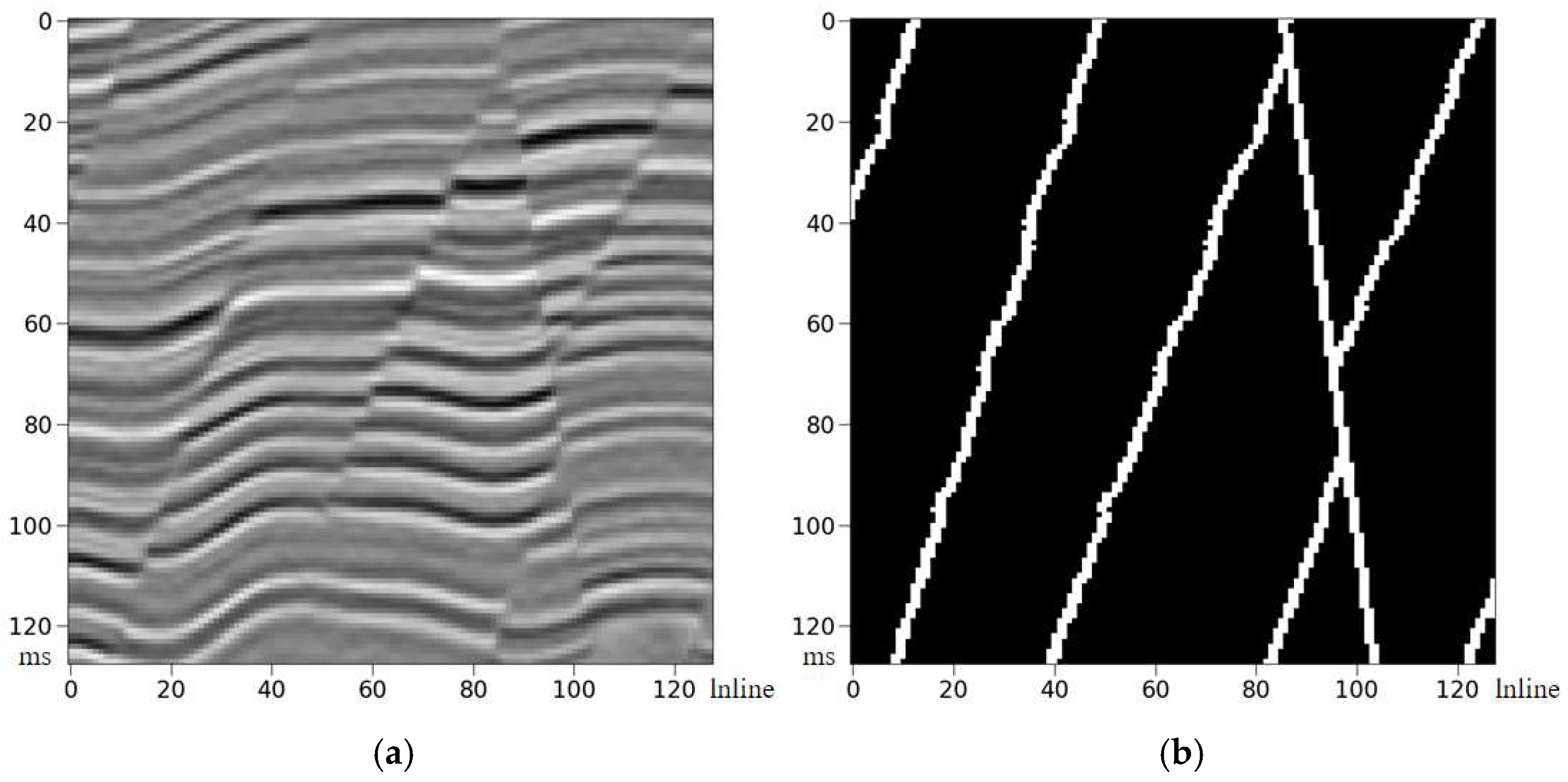
The dataset used in this paper is the synthetic seismic record dataset provided by [17] as an open-source resource. There are a total of 600 two-dimensional synthetic seismic records along with their corresponding label data. Each data has a size of 128 × 128. Figure 3 shows the synthetic seismic records and the corresponding label data.

Meanwhile, in order to increase the diversity and complexity of the data and enhance the generalization ability of the model, before training, data augmentation processing was carried out on the dataset. Synthetic seismic records and their corresponding label data were rotated by 90, 180, and 270 degrees clockwise to make the dataset more diverse.

Due to the non-stationarity of the seismic data, there are significant differences in amplitude values. Moreover, in order to improve the quality of the dataset, before using the dataset for training, the data was normalized and its value range was mapped to the interval [0, 1]. The calculation formula is as follows:

$$X_{norm}={\displaystyle \frac{X-X_{\min }}{X_{\max }-X_{\min }}}$$

(1)

In the formula, $X$ represents the original data, $X_{\min }$ represents the minimum value of the original data, $X_{\max }$ represents the maximum value of the original data, and $X_{norm}$ represents the normalized data.

3.2. Loss Function and Evaluation Metrics

The loss function is a core component in deep learning, used to measure the discrepancy between the predicted values of the model and the original values, providing a clear objective for model optimization. Since the problem to be solved in this article is a binary classification problem, the loss function used is the BCE (binary cross-entropy) loss function, which is:

$$BCE=-{\displaystyle \frac{1}{N}}{\displaystyle \sum _{i=1}^N((y_i\log (f(x_i)))}+(1-y_i)\log (1-f(x_i)))$$

(2)

In the formula, $y$ represents the true label, $f(x)$ represents the predicted probability value, and $N$ represents the sample quantity. The binary cross-entropy loss function can only be used for binary classification problems. It is usually used in combination with the Sigmoid activation function to compress the output to the range of [0, 1]. In the case of fault detection, the output of the network model usually contains only one probability value. This value indicates whether a fault exists or not. The closer the probability value is to 1, the higher the likelihood that there is a fault.

Evaluation metrics are also a core component in deep learning, used to quantify the performance of the model and provide an objective basis for model selection, optimization, and deployment. The evaluation metric selected for this article is accuracy. Accuracy is the most intuitive evaluation index for classification models, representing the proportion of correctly predicted samples by the model among the total samples. Its calculation formula is:

$$Accurary={\displaystyle \frac{TP+TN}{TP+TN+FP+FN}}$$

(3)

In the formula, $TP$ represents the positive samples that were correctly predicted (originally positive and predicted as positive), $TN$ represents the negative samples that were correctly predicted (actually negative and predicted as negative), $FP$ represents the false alarms (actually negative and predicted as positive), $FN$ and represents the missed detections (actually positive and predicted as negative).

3.3. Model Training

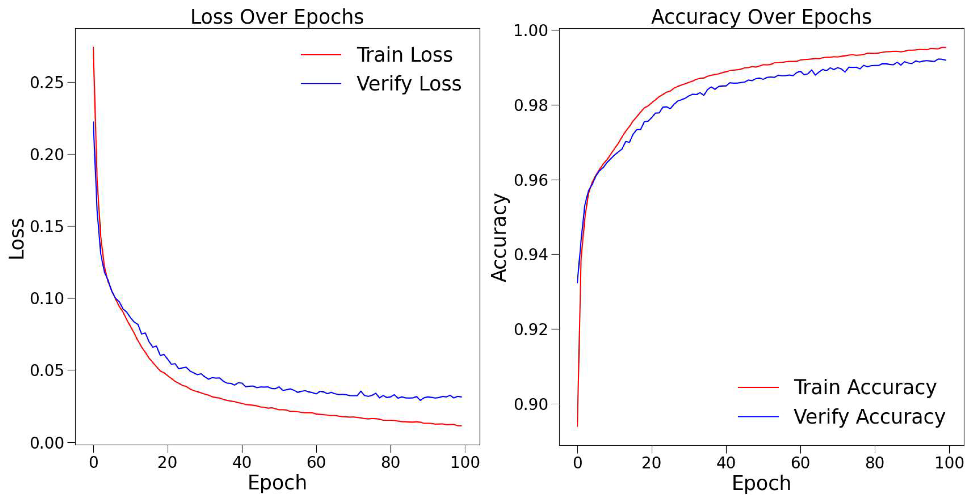
The model training is conducted using the aforementioned generated dataset, and the dataset is subjected to data augmentation and normalization processing. Before training, the dataset is divided into training set, validation set and test set in a ratio of 8:1:1. The training set is used to train the network model and adjust the weights of the network model; the validation set is used to adjust the hyperparameters of the network model to prevent overfitting; the test set is used to verify the generalization ability of the network model for unknown data. In terms of the selection of network hyperparameters, the initial learning rate is set to 0.0001. Setting the learning rate too high can prevent the model from converging during training, while setting it too low can result in extremely slow convergence and a tendency to become stuck in local optima. Due to the unique adaptive learning rate mechanism of the Adam optimizer, there is no need to frequently adjust the learning rate during the training process. Therefore, the Adam optimizer is chosen as the optimizer for the network model; Since fault identification in seismic data is a binary classification problem, Therefore, the binary cross-entropy loss function is selected as the loss function for the network model; the total number of iterations is 100, the batch size is 8, and the network model is trained formally on a GPU-GTX1060 with 6 GB of video memory. The total training time was 1825 s. The changes in the loss function and accuracy rate are shown in Figure 4.

As can be seen from the figure, during the iterative process, the loss function values of both the training set and the validation set gradually converge. In the final iterative process, the loss function values of both the training set and the validation set converge to a stable value, indicating that the network model has been trained to its optimal state. Meanwhile, during the iterative process, the accuracy values of both the training set and the validation set gradually increased, indicating that the model is gradually learning and also helping us identify any anomalies during the training process.

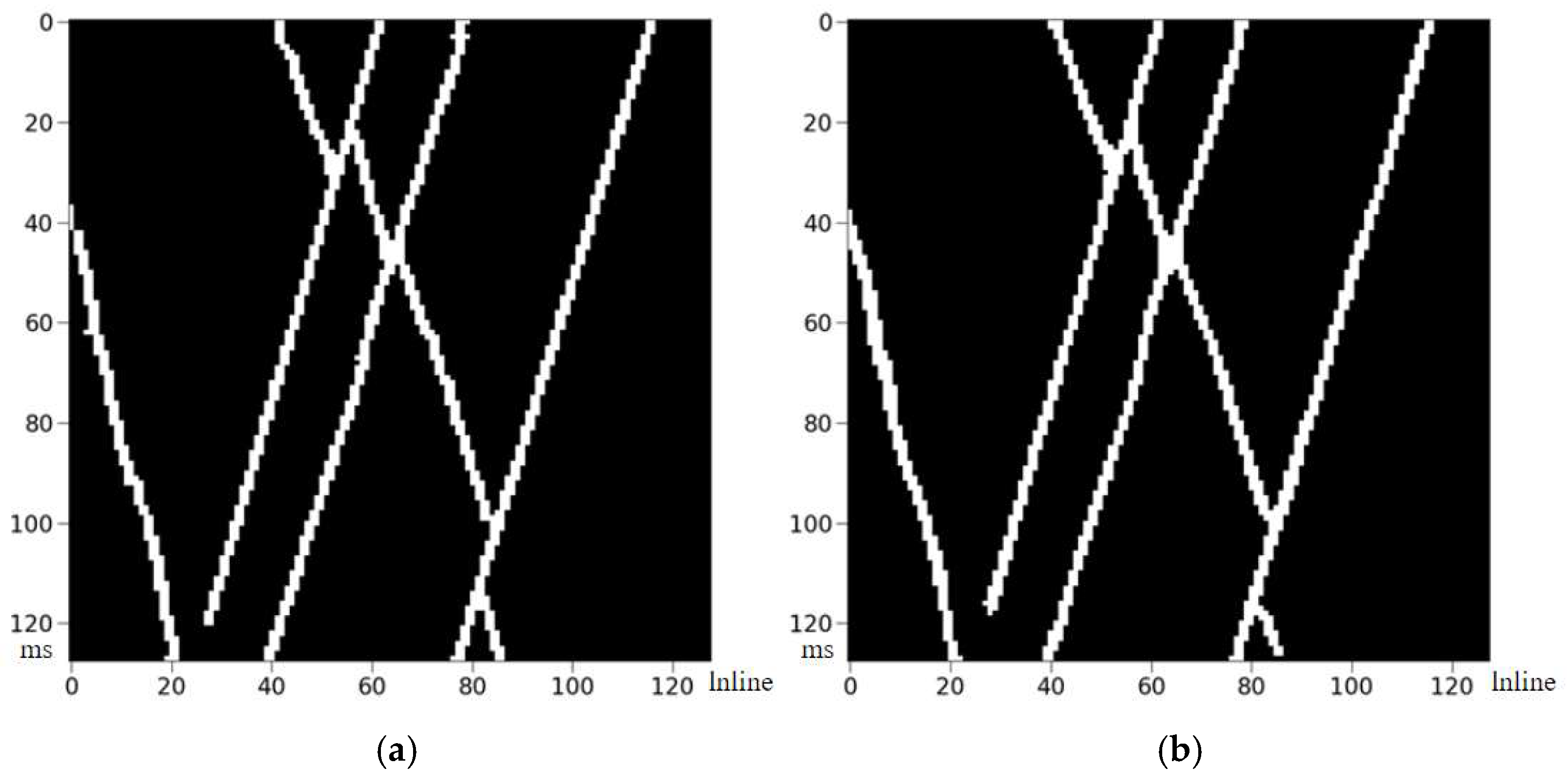
To test the generalization performance of the network model, a synthetic seismic data was randomly selected from the test set as the input, and the predicted fault data by the model was finally output. The specific results are shown in Figure 5. Overall, the predicted fault data has a high degree of similarity with the labeled data, which verifies the effectiveness of the network model proposed in this paper.

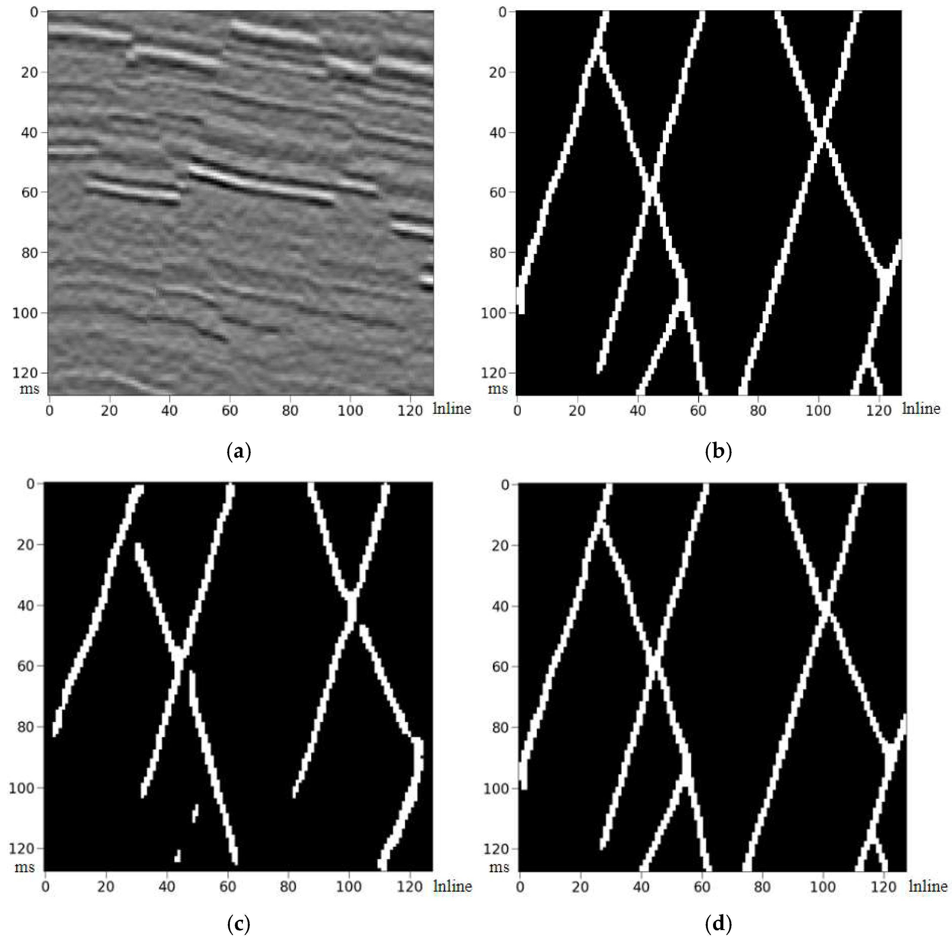
To highlight the effectiveness of the network in this paper, during the training process, a U-Net network model was also trained using the same method. Again, a synthetic seismic data was randomly selected from the test set as the input. The SEU-Net network model and the U-Net network model were, respectively, used for prediction, and the predicted tomographic data of the models were obtained. Specifically, as shown in Figure 6.

As can be seen from the figure, the continuity of the tomographic data predicted by the U-Net network model is poor, and its similarity to the label data is low. However, the tomographic data predicted by the SEU-Net network model has better continuity and is highly similar to the label data. This further validates the effectiveness of the network model proposed in this paper.

Meanwhile, to avoid randomness, the SEU-Net network model and the U-Net network model were, respectively, used to make predictions for the entire test set, and the accuracy, recall, F1-score, and IoU was calculated. To avoid chance factors, 10 predictions were made on the test set, and the average of the metric values from these 10 predictions was calculated. The results are shown in

Table 1. Comparison of the accuracy rates of different network models.

Type of Network	Accuracy Rate	Recall	F1-Score	IoU
U-Net	0.9623	0.9611	0.9614	0.9602
SEU-Net	0.9856	0.9821	0.9853	0.9747

.

As can be seen from the table, the prediction accuracy of the SEU-Net network model in the entire test set is higher than that of the U-Net network model, indicating that the SEU-Net network model has stronger generalization ability and can better identify faults.

3.4. Original Data

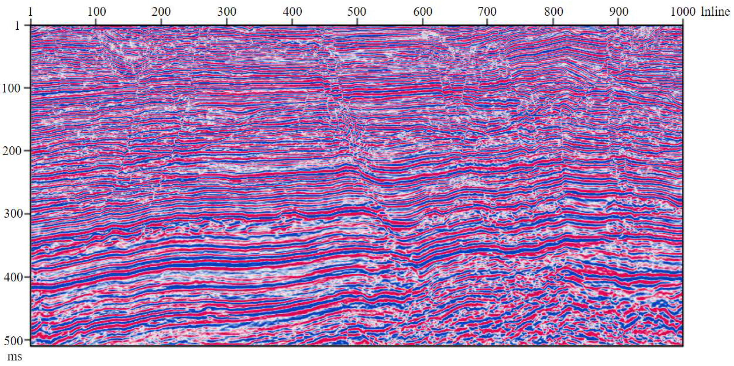
In order to detect the effect of the network in identifying faults in original seismic data, a two-dimensional original seismic data with a size of 1000 × 512 from a certain region was selected (as shown in Figure 7), and the network model trained in the previous section was used to make predictions on this data.

Since the size of the original seismic data is inconsistent with the input requirements of the network model, it is impossible to directly carry out predictions on the original seismic data. Therefore, it is advisable to consider using the sliding sampling method to predict the original seismic data. Since the input size of the network model is 128 × 128, a window of the same size (128 × 128) can be used to perform sliding prediction on the original seismic data. The specific operation is as follows: Firstly, fill the original seismic data to make its size a multiple of 128, and fill the remaining part with 0 values. At this point, the size of the original seismic data is 1024 × 512. Then, use a sliding window of size 128 × 128 on the original seismic data for sliding, with a stride of 128. This way, 32 original seismic data points of size 128 × 128 can be obtained. Finally, we use the trained network model to make predictions in the order of sliding sampling, thereby obtaining the predicted fault data and removing the filled parts to obtain the final output result.

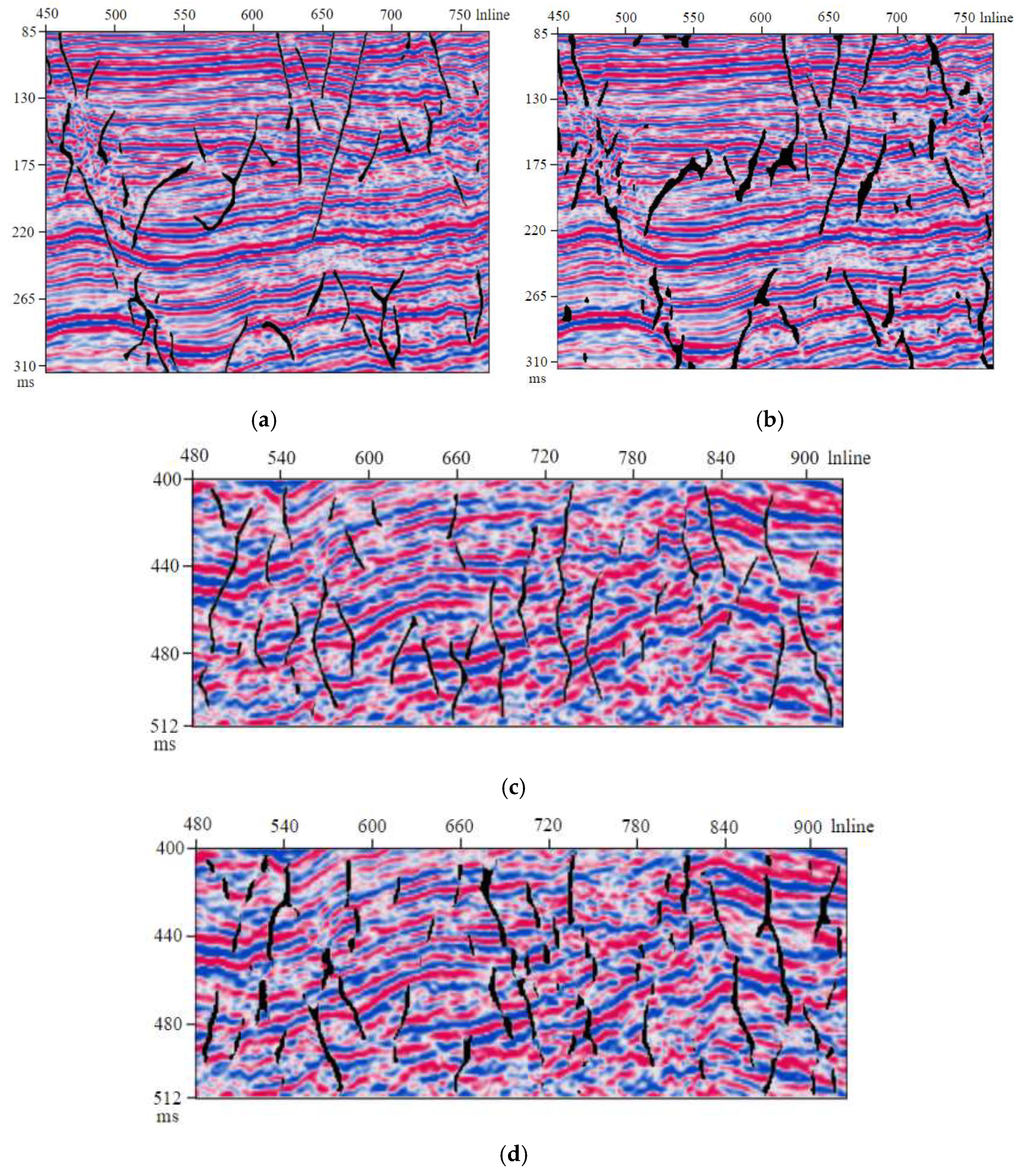
According to the above method, the SEU-Net network model and the U-Net network model are, respectively, used to predict the original seismic data. In order to better display the prediction effect, two small pieces of data with different scales are selected from the fault prediction results of the original seismic data for display. The results are shown in Figure 8. It can be seen from the figure that both networks can predict the faults, but the faults predicted by the SEU-Net network model are more refined and have better continuity. This indicates that the network model in this paper can also achieve good application effects on original seismic data and can be applied in practice.

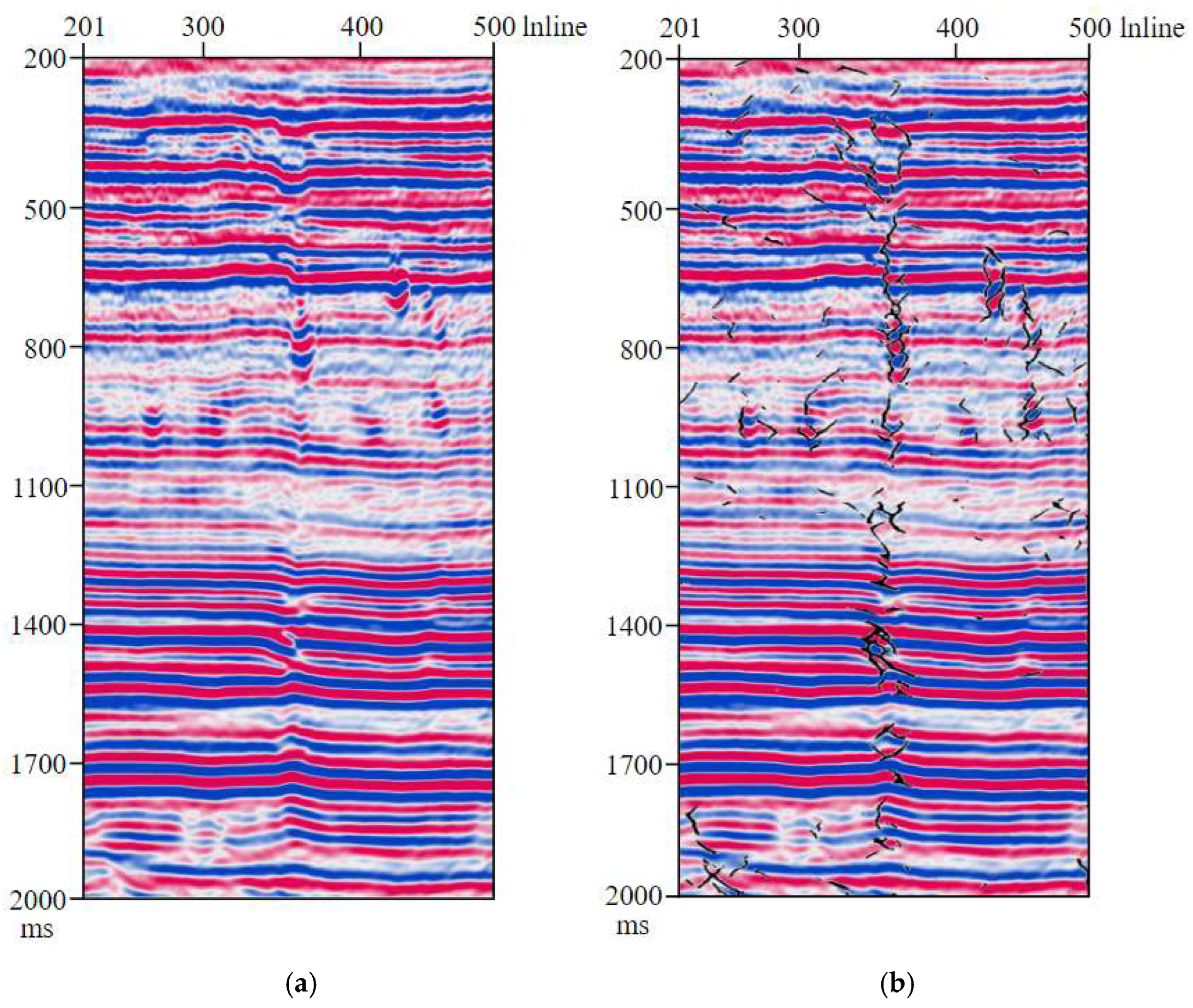
To further verify the performance of the SEU-Net network model, seismic data from Shunbei Oilfield in western China (as shown in Figure 9a) was selected for testing. The faults in this area are mainly strike-slip faults, and the prediction results are shown in Figure 9b.

It can be seen from the prediction results that the predicted fault positions are accurate and have good continuity, indicating that the network model proposed in this paper can also achieve good application effects in different original seismic data and has good applicability.

4. Conclusions

Based on the original U-Net network, this paper introduces the SE block into the U-Net network and proposes a SEU-Net network model for fault identification of seismic data. The experimental results of this paper show that the SEU-Net network model has higher prediction accuracy than the original U-Net network model and can effectively identify faults in seismic data.

However, the study has certain limitations. Due to the introduction of the SE attention module, the computational complexity of the SEU-Net model is higher than that of the standard U-Net. The training process on a GTX1060 GPU for two-dimensional data of size 128 × 128 took approximately 1825 s for 100 epochs. This implies that applying the model to larger 2D sections or 3D seismic volumes in real-world projects would require significant computational resources and time, which is a crucial practical constraint.

Therefore, due to the influence of computing power and training time, the network model in this paper was only applied to two-dimensional seismic data and achieved good results, which also indicates that the faults predicted by this network model are valid. Additionally, consideration will be given to incorporating other architectures into the network model to improve its ability to extract features and fit data, thereby achieving further enhancement. Specific strategies include:

• Structural Optimization: Exploring lightweight network designs, such as using more efficient channel attention mechanisms or reducing redundant feature channels, to lower computational complexity.
• Hardware Acceleration: Utilizing more powerful hardware resources (e.g., multi-GPU clusters or TPUs) and distributed training frameworks to accelerate the training process for large-scale data.
• Efficient Inference: Researching methods like model pruning and quantization to reduce the model’s memory footprint and computational cost during deployment, facilitating practical application.

Furthermore, to enhance the model’s robustness in processing high-noise seismic data—a common challenge in real-world applications—the architecture requires further targeted improvements. The current SE module excels at channel-wise feature recalibration but is less effective in explicitly suppressing spatial noise. The limitations of the current architecture and prospective solutions for future research are summarized in

Table 2. Limitations and prospective improvements of the SEU-Net architecture for high-noise seismic data processing.

Current Limitation	Impact on High-Noise Data Processing	Proposed Improvement
Sensitivity of SE Blocks to Feature Quality	Noisy features are squeezed and excited alongside clean features, potentially amplifying noise in certain channels.	Integrate a Spatial-Channel Concurrent Attention mechanism.
Limited Multi-scale Context Capture	The U-Net backbone may lose subtle fault features amidst strong noise, as small faults can be easily obscured.	Incorporate an Atrous Spatial Pyramid Pooling (ASPP) module in the bottleneck.
Fixed Feature Extraction	The standard convolutional kernels are static after training and may not adapt optimally to varying local noise conditions.	Replace standard convolutions with Dynamic Convolutions or Attention-augmented Convolutions.

below.

The implementation of these advanced architectural improvements, combined with the extension to 3D, will be the focus of our subsequent research. This dual pathway of enhancing model architecture and expanding data dimensionality is expected to yield a more powerful, robust, and universally applicable tool for automated seismic fault interpretation under challenging conditions.

Due to the improvement in computing power, it is possible to consider directly using 3D seismic datasets to train the network. At the same time, in order to adapt to 3D seismic datasets, modifications need to be made to the network structure to enable it to train on 3D seismic data. This can further simplify the prediction process, allowing direct prediction on 3D seismic data volumes, greatly improving prediction efficiency.

References

1. Zhang, L.X.; GAO, J.T.; MA, Q.; Yang, R.T.; Wang, Z.B.; Li, F. Research on Seismic Fault Identification Methods Based on Improved UNet++. Comput. Technol. Dev. 2023, 33, 199–205+213. [Google Scholar]
2. Alohali, R.; Alzubaidi, F.; Van Kranendonk, M.; Clark, S. Automated fault detection in the Arabian Basin. Geophysics 2022, 87, IM101–IM109. [Google Scholar] [CrossRef]
3. Gao, K.; Huang, L.J.; Zheng, Y.C. Fault detection on seismic structural images using a nested residual U-Net. IEEE Trans. Geosci. Remote Sens. 2022, 60, 4502215. [Google Scholar] [CrossRef]
4. Gao, K.; Huang, L.J.; Zheng, Y.C.; Lin, R.R.; Hu, H.; Cladohous, T. Automatic fault detection on seismic images using a multiscale attention convolutional neural network. Geophysics 2021, 87, N13–N29. [Google Scholar] [CrossRef]
5. Zhou, R.S.; Yao, X.M.; Hu, G.M.; Yu, F.C. Learning from unlabelled real seismic data: Fault detection based on transfer learning. Geophys. Prospect. 2021, 69, 1218–1234. [Google Scholar] [CrossRef]
6. Zhu, D.L.; Li, L.; Guo, R.; Tao, C.F.; Zhan, S.F. 3D fault detection: Using human reasoning to improve performance of convolutional neural networks. Geophysics 2022, 87, IM143–IM156. [Google Scholar] [CrossRef]
7. Di, X.; Liu, Y. Research progress of deep learning in seismic fault interpretation. Prog. Geophys. 2025, 40, 1688–1716. [Google Scholar]
8. Bahorich, M.; Farmer, S. 3-D seismic discontinuity for faults and stratigraphic features: The coherence cube. Lead. Edge 1995, 14, 1053–1058. [Google Scholar] [CrossRef]
9. Yang, G.Q.; Liu, Y.L.; Zhang, H.W. The calculation method of curvature attributes and its effect analysis. Prog. Geophys. 2015, 30, 2282–2286. [Google Scholar]
10. Ma, Y.X.; Li, H.L.; Liu, K.Y.; Gu, H.M.; Ren, H. Application of an ant-tracking technique based on spectral de-composition to fault characterization. Geophys. Prospect. Pet. 2020, 59, 258–266. [Google Scholar]
11. Pedersen, S.I.; Randen, T.; Sonneland, L.; Steen, Ø. Automatic fault extraction using artificial ants. In SEG Technical Program Expanded Abstracts; Society of Exploration Geophysicists: Salt Lake City, UT, USA, 2002; pp. 107–116. [Google Scholar]
12. Wu, T.R.; Gao, J.H.; Chang, D.K.; Wang, H.L.; Tao, H.F.; Li, M.Y. Faults identification of seismic data based on Transformer. Oil Geophys. Prospect. 2024, 59, 1217–1224. [Google Scholar]
13. Jing, J.K.; Yan, Z.; Zhang, Z.; Gu, H.M.; Han, B.K. Fault detection using a convolutional neural network trained with point-spread function-convolution-based samples. Geophysics 2023, 88, IM1–IM14. [Google Scholar] [CrossRef]
14. Di, H.B.; Wang, Z.; AlRegib, G. Why using CNN for seismic interpretation? An investigation. In Proceedings of the SEG International Exposition and Annual Meeting, Anaheim, CA, USA, 14–19 October 2018; pp. 2216–2220. [Google Scholar]
15. Chen, L.; Xiao, C.B.; Yu, J.; Wang, Z.L.; Li, X.L. Fault recognition based on affinity propagation clustering and principal component analysis. Oil Geophys. Prospect. 2017, 52, 826–833. [Google Scholar]
16. Huang, L.; Dong, X.S.; Clee, T.E. A scalable deep learning platform for identifying geologic features from seismic attributes. Lead. Edge 2017, 36, 249–256. [Google Scholar] [CrossRef]
17. Wu, X.M.; Liang, L.M.; Shi, Y.Z.; Sergey, F. FaultSeg3D: Using synthetic data sets to train an end-to-end convolutional neural network for 3D seismic fault segmentation. Geophysics 2019, 84, IM35–IM45. [Google Scholar] [CrossRef]
18. Wu, X.M.; Shi, Y.Z.; Fomel, S.; Liang, L.M.; Zhang, Q.; Yusifov, A.Z. FaultNet3D: Predicting Fault Probabilities, Strikes, and Dips With a Single Convolutional Neural Network. IEEE Trans. Geosci. Remote Sens. 2019, 57, 9138–9155. [Google Scholar] [CrossRef]
19. Liu, N.H.; He, T.; Tian, Y.J.; Wu, B.Y.; Gao, J.H.; Xu, Z.B. Common-azimuth seismic data fault analysis using residual UNet. Interpretation 2020, 8, SM25–SM37. [Google Scholar] [CrossRef]
20. Tang, Z.X.; Wu, B.Y.; Wu, W.H.; Ma, D.B. Fault detection via 2.5D transformer U-Net with seismic data pre-processing. Remote Sens. 2023, 15, 1039. [Google Scholar] [CrossRef]
21. Zhang, Z.; Yan, Z.; Gu, H.M. Automatic fault recognition with residual network and transfer learning. Oil Geophys. Prospect. 2020, 55, 950–956. [Google Scholar]
22. Chang, D.K.; Yong, X.S.; Wang, Y.H.; Yang, W.Y.; Li, H.S.; Zhang, G.Z. Seismic fault interpretation based on deep convolutional neural networks. Oil Geophys. Prospect. 2021, 56, 1–8. [Google Scholar]
23. Liu, G.X.; MA, Z.H. Fault Identification of Post Stack Seismic Data by Improved Unet Network. Chin. J. Comput. Phys. 2023, 40, 742–751. [Google Scholar]
24. Gao, X.C.; Liang, Y.H.; Wang, L.L.; WU, J.Z. Three-dimensional fault identification using RAtte-UNet. Oil Geophys. Prospect. 2025, 60, 12–20. [Google Scholar]
25. Wu, X.M.; Geng, Z.C.; Shi, Y.Z.; Pham, N.; Fomel, S.; Caumon, G. Building realistic structure models to train convolutional neural networks for seismic structural interpretation. Geophysics 2020, 85, WA27–WA39. [Google Scholar] [CrossRef]
26. Guarido, M.; Wozniakowska, P.; Emery, D.J.; Lume, M.; Trad, D.O.; Innanen, K.A. Fault detection in seismic volumes using a 2.5D residual neural networks approach. In Proceedings of the First International Meeting for Applied Geoscience & Energy Expanded Abstracts, Denver, CO, USA, 26 September–1 October 2021; pp. 1626–1629. [Google Scholar]
27. Li, S.J.; Gao, J.H.; Gui, J.Y.; Wu, L.K.; Liu, N.H.; He, D.Y.; Guo, X. Fully connected U-Net and its application on reconstructing successively sampled seismic data. IEEE Access 2023, 11, 99693–99704. [Google Scholar] [CrossRef]
28. Lin, L.; Zhong, Z.; Cai, Z.X.; Sun, A.Y.; Li, C.L. Automatic geologic fault identification from seismic data using 2.5D channel attention U-Net. Geophysics 2022, 87, IM111–IM124. [Google Scholar] [CrossRef]
29. Wu, W.H.; Yang, Y.; Wu, B.Y.; Ma, D.B.; Tang, Z.X.; Yin, X. MTL-FaultNet: Seismic data reconstruction assisted multitask deep learning 3-D fault interpretation. IEEE Trans. Geosci. Remote Sens. 2023, 61, 5914815. [Google Scholar] [CrossRef]
30. Ronneberger, O.; Fischer, P.; Brox, T. U-net: Convolutional networks for biomedical image segmentation. In Proceedings of the 18th International Conference on Medical Image Computing and Computer-Assisted Intervention—MICCAI 2015 Part III, Munich, Germany, 5–9 October 2015; pp. 234–241. [Google Scholar]
31. Hu, J.; Li, S.; Sun, G. Squeeze-and-excitation networks. In Proceedings of the IEEE conference on computer vision and pattern recognition, Salt Lake City, UT, USA, 18–22 June 2018; pp. 7132–7141. [Google Scholar]
Figure 1. SEU-Net network structure. (The numbers in the figure represent the number of channels in the feature map).
Applsci 15 10152 g001
Figure 2. Squeeze-and-excitation block structure. (In the figure, H, W, and C represent the dimensions of the feature tensor, Fsq represents the squeeze operation, Fex represents the excitation operation, and Fscale represents the weighted operation).
Applsci 15 10152 g002
Figure 3. Synthetic data diagram; (a) Sample data (b) Label data.
Applsci 15 10152 g003
Figure 4. Loss function and accuracy rate change diagram.
Applsci 15 10152 g004
Figure 5. Comparison chart of prediction results and label data. (a) Label data. (b) SEU-Net network model prediction results.
Applsci 15 10152 g005
Figure 6. Comparison of different network model predictions; (a) Sample data; (b) Label; (c) U-Net network model prediction results; (d) SEU-Net network model prediction results.
Applsci 15 10152 g006
Figure 7. Two-dimensional original seismic data.
Applsci 15 10152 g007
Figure 8. Original seismic data fault detection results; (a) SEU-Net network model prediction results; (b) U-Net network model prediction results; (c) SEU-Net network model prediction results; (d) U-Net network model prediction results.
Applsci 15 10152 g008
Figure 9. Original seismic data fault detection results (Data from Shunbei Oilfield, Tarim Basin); (a) Original seismic data (b) SEU-Net network model prediction.
Applsci 15 10152 g009