Abstract
Soil–rock mixtures pose significant challenges in mountainous regions due to their complex flow behavior and destructive potential during landslides and debris flows. Despite growing interest in using baffle arrays as protective measures, current research has focused on idealized soil or rock materials, leaving a notable gap in understanding their efficacy against heterogeneous soil–rock mixtures under varied slope and baffle configurations. This study employs the Material Point Method to simulate the continuum behavior of the soil matrix, while the Discrete Element Method (DEM) models the discrete dynamics of rock boulders. By incorporating Spheropolygon DEM, the model accurately captures complex soil–rock structure interactions. Parametric simulations are conducted to evaluate the effects of baffle location and slope angle on flow kinematics, impact forces, and energy dissipation. Results show that baffles placed closer to the structure significantly reduce downstream impact forces and kinetic energy by enhancing energy dissipation. Steeper slope angles result in increased impact forces on the structure due to greater conversion of potential energy to kinetic energy. The findings provide quantitative insights into optimizing baffle placement for improving infrastructure resilience against soil–rock mixture flows.
1. Introduction
Soil–rock mixtures, which consist of high-strength rock blocks within a fine-grained soil matrix, pose significant challenges in geotechnical engineering [1,2]. Geological hazards associated with soil–rock mixtures, such as landslides and debris flows, represent considerable threats to both human life and infrastructure [3,4], particularly in mountainous terrains. Given the potentially catastrophic impacts of such disasters, the development of effective mitigation strategies to reduce these risks is critical. Among these strategies, the use of baffles has emerged with increasing attention due to their effectiveness in reducing the destructive potential of soil–rock mixture flows [5,6]. The feasibility of implementing large-scale baffle arrays is often limited by significant logistical challenges inherent to remote and rugged mountainous terrain. These practical hurdles, including the transportation of heavy materials and construction equipment to inaccessible sites, directly result in substantially higher project costs [7,8]. These practical limitations underscore the importance of developing optimized design strategies that maximize protective efficiency while minimizing construction demands.
Numerous researchers have conducted small-scale flume experiments to explore the effects of various baffle configurations on geohazardous flows [9,10,11]. Ng et al. [12] investigated the influence of baffle parameters, including height, number of rows, spacing, and transverse blockage, on landslide movement through physical flume tests. Their results indicated that taller baffles, staggered multiple-row arrangements, and optimal spacing reduced run-out distances and overflow volumes. Bi et al. [13] investigated optimal baffle layouts for enhancing the blocking efficiency of rock avalanches, demonstrating that full-coverage, multi-row configurations reduced the risk of particle splashing. Kim et al. [14] showed that cylindrical baffles dissipated energy more efficiently than rectangular ones, with taller baffles resulting in lower downstream velocities and flow depths due to intensified jet–flow interactions. However, a fundamental limitation of small-scale flume experiments is that dimensionless parameters governing debris flow behavior cannot be simultaneously scaled to match both the model and the prototype. In addition, boundary effects imposed by the flume walls may artificially modify flow dynamics, thereby limiting the direct applicability of laboratory observations to natural settings [15].
Numerical simulation is a crucial method for investigating the complex dynamics between geohazardous flows and protective baffles [16,17,18]. Traditional grid-based techniques, such as the Finite Element Method (FEM), are commonly applied in engineering practice. Ozbay and Cabalar [19] used FEM to study slope stability under varying groundwater conditions. However, FEM faces difficulties in accurately modeling the large deformations and discontinuities characteristic of soil–rock mixtures [20]. To address these limitations, particle-based methods have been introduced. The Particle Finite Element Method (PFEM) is well-suited to geotechnical problems involving large displacements [21], such as flow-like landslides. Zhang et al. [22] employed PFEM to examine the kinematics of sliding masses and assess how factors such as material density, slip surface geometry, and roughness influence final deposition patterns. Another widely used particle-based approach is Smoothed Particle Hydrodynamics (SPH), which has gained popularity due to its ability to accurately track free-surface flows [23]. A major advantage of SPH is its natural adaptability to large continuum deformations, thereby avoiding the mesh entanglement issues often encountered in FEM [24]. Yang et al. [25] used SPH to simulate granular flow interactions with rigid structures like baffles and check dams, revealing flow deceleration mechanisms and optimizing baffle design. However, SPH poses challenges in boundary condition treatment [26]. In contrast, the Material Point Method (MPM) is particularly suitable for modeling materials undergoing large deformations and generally offers greater computational efficiency [27]. Li et al. [28] employed MPM to analyze the influence of baffle arrangement on debris flow behavior and deposition characteristics. Despite these valuable studies using methods like SPH and MPM, they have typically focused on flows composed solely of either soil or rock, without specifically addressing the unique characteristics and behavior of soil–rock mixtures.
Addressing the complex interactions between heterogeneous soil–rock mixtures and protective structures requires advanced numerical techniques, leading to the development of coupled methodologies [29]. Bi et al. [30] coupled Computational Fluid Dynamics (CFD) with the Discrete Element Method (DEM) to investigate debris flow interactions with slit dams, focusing on the effects of water content and slope angle. Other studies have employed the SPH-DEM coupling method to model the behavior of debris flow constituents and improve predictions of critical parameters such as flow velocity and impact forces [5,31]. The coupling approach has also been extended to the MPM and DEM, which has been applied to a range of geotechnical problems, including granular impact dynamics [32], anchor pullout analysis [33], and the assessment of bearing capacity in anisotropic soils [34]. Specifically concerning impact dynamics, Ren et al. [35] proposed an MPM–DEM scheme to examine how variations in boulder content influence impact forces and kinetic energy, providing valuable insights into the destructive power of these heterogeneous flows and the effectiveness of protective measures. Li et al. [36] further investigated the performance of baffle structures under complex soil–rock flow conditions. It should be noted that the fluid phase can substantially modify both the mobility of the flow and the magnitude of the resulting impact forces [37,38], and the impact of the water phase cannot be neglected. While these studies have contributed to understanding interaction mechanisms, the specific influence of baffle positioning on protective performance against soil–rock mixture flows with different slope angles remains insufficiently explored. To address this gap, this study employs a coupled MPM-DEM approach to investigate the influence of baffle location on protective efficiency. In this framework, the MPM is used to model the continuous behavior of the soil matrix, while the DEM captures the discrete dynamics of rock particles. To further enhance the representation of structural response, the Spheropolygon DEM (SDEM) is incorporated, allowing for accurate simulation of complex soil–rock structure interactions.
This paper is structured as follows: Section 2 provides a concise overview of the MPM, DEM, and the coupling scheme. Section 3 presents the numerical simulation setup, including model geometry, material parameters, and the parametric design involving variations in baffle location and slope angle. Section 4 discusses the simulation results in detail, focusing on the effects of baffle placement and slope angle on impact forces, flow dynamics, and energy dissipation. Finally, Section 5 summarizes the main findings and highlights the practical implications for the design of mitigation structures against soil–rock mixture flows.
2. Numerical Scheme
2.1. MPM Method for Soil Particles
The MPM, which originated from the Fluid Implicit Particle (FLIP) method, is a hybrid numerical technique [39,40]. It uses Lagrangian material points to track the state and history of the material while employing an Eulerian background grid to solve the equations of motion, offering advantages in handling extremely large deformations and complex material behavior without encountering mesh distortion issues [41]. The mass conservation equation and momentum balance equation can be expressed as:
where , , , m and refer to the material density, velocity, Cauchy stress, body force, and coupled force. In this study, the updated stress last explicit time integration scheme is adopted to solve these governing equations. The computational process begins at time t:
using the shape function and its gradient , physical quantities associated with material points, such as mass , velocity , contact force , body force , and internal force , are projected onto the computational grid to obtain the corresponding nodal quantities: nodal mass , velocity , external force , and internal force . Here, , , and denote the volume, Cauchy stress, and body force at the material point, respectively.
Since MPM is a Lagrangian method, the mass conservation equation is inherently satisfied. Therefore, only the momentum balance equation needs to be explicitly solved on the background grid:
At this stage, boundary conditions are applied to the computational grid to determine the nodal quantities [42]. is the damping force, and is the damping coefficient. Subsequently, using the time step , these updated nodal values are then interpolated back to the particles to update their physical variables, such as position, velocity, and stress:
where represents the velocity gradient tensor at particle p and time t, is the identity tensor, denotes the initial particle volume, is the strain rate tensor, and is the rotation rate tensor. refers to the elastoplastic modulus tensor, which is determined by the selected constitutive model. In this study, the Mohr–Coulomb (MC) constitutive model is adopted to characterize the mechanical behavior of soils, as it effectively captures the frictional and dilatant nature of geomaterials [43].
2.2. Discrete Element Method
DEM is a widely employed technique for simulating the motion of individual particles [44,45]. However, classical DEM typically represents particles as spheres, which limits its ability to accurately model irregularly shaped objects. To address this limitation, the SDEM has been developed, allowing for the representation of irregular particle geometries. Mathematically, a spheropolygon is defined as the Minkowski sum of a polygon and a disk with a specified radius [46]. This formulation introduces an elastic boundary around the polygon, enabling more realistic contact force calculations by accounting for particle shape irregularities [47]. The dynamic behavior is described by the following equations [48]:
where is the mass of the DEM particle, and represents its translational velocity. The moment of inertia tensor is given by , while is the angular velocity. The gravitational force acting on the particle is expressed as . The term represents the torque generated by the contact force between DEM particles, while represents the torque resulting from the coupling force exchanged with the MPM solver.
2.3. Coupling Scheme Between MPM and DEM
Collision detection and contact force computation are two critical components of the MPM–DEM coupling scheme. The collision detection process utilizes the MPM background grid as a linked-cell structure to identify potential interactions between MPM points and DEM particles. Once the potential contact is identified, as illustrated in Figure 1, the MPM points are temporarily treated as DEM particles, allowing the contact forces to be calculated within the unified DEM framework. The Hertz–Mindlin contact model is employed to calculate both normal and tangential contact forces between interacting particles. The equations for these contact forces are provided below:
where and are the normal and tangential contact forces, respectively. , , and are the equivalent Young’s modulus, contact radius, and mass. and represent the normal and tangential overlaps. and are the relative normal and tangential velocities, and are stiffness coefficients, is the damping coefficient, and is the friction coefficient.
where e is the coefficient of restitution, is the equivalent shear modulus. It is important to note that when computing contact forces between different DEM particles, the same formulations as given in Equations (19) and (20) are applied. However, when determining the equivalent material properties (, , , and ), the physical parameters of each interacting particle should be selected based on their material characteristics.
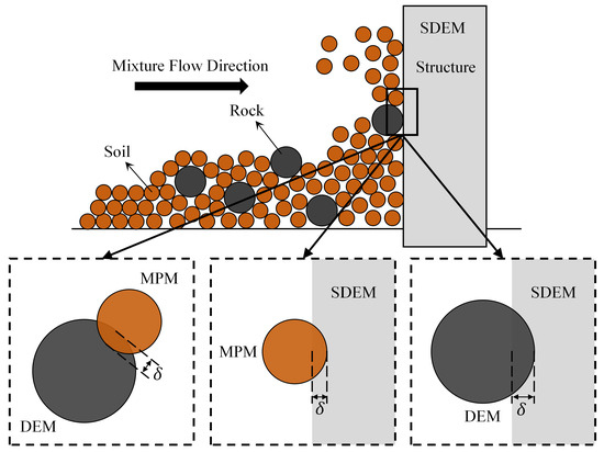
Figure 1.
Coupling scheme between different methods.
A detailed description of the MPM-DEM coupling scheme can be summarized as follows:
- Collision Detection: Potential contact pairs are identified by employing the MPM node-based linked-cell structure.
- Force Calculation: Contact forces are computed using the Hertz–Mindlin model, effectively treating the MPM points as discrete DEM particles for this step.
- MPM Process: The calculated coupled force is subsequently added as an external force term to the MPM governing equations (Equations (1) and (2)). The motion of the MPM points is then solved using the same computational procedures detailed in Section 2.1.
For this coupling approach, the integration of both MPM and DEM solutions is performed using explicit schemes, with both components adopting a shared time step [32]. Numerical stability is maintained by constraining the global time step according to the Courant–Friedrichs–Lewy (CFL) condition:
In this equation, is the Courant number, h is the initial size of the material point, c denotes the speed of sound, m represents the DEM particle mass, and is the contact normal stiffness. Specifically, the first term in Equation (24) is associated with the MPM, while the second term corresponds to the DEM component [42]. To optimize the utilization of high-performance computing resources, parallel algorithms for the MPM and DEM modules have been developed within the in-house ComFluSoM library, employing an MPI/OpenMP framework.
Interactions at the soil–rock interface in the coupled model are represented using the Hertz–Mindlin contact formulation. Momentum exchange is computed through normal and tangential contact forces derived from particle overlap and material properties. However, under extreme flow regimes, certain processes such as particle breakage and fragmentation are not considered in the present model.
It is worth noting that the numerical framework has been partially validated through comparisons with established experiments in the author’s previous works [35,49]. In particular, the soil–structure interaction was verified against the dry granular flow impact tests of Moriguchi et al. [50], where the model reproduced the forces on rigid baffle-like structures. In addition, soil–boulder interaction was examined through projectile impact simulations into a granular medium, showing close agreement with the experiments of Ciamarra et al. [51]. These validations of fundamental interactions provide confidence in the model’s ability to capture the more complex coupled processes investigated in this study.
3. Numerical Simulations and Results
Figure 2 illustrates the simplified numerical model setup used in this study, which includes the rock–soil mixture, baffles, structure, and terrain. In this configuration, the rock–soil mixture is initially located in the upstream section of the flume, while the structure is positioned in the downstream section. The baffle is strategically placed between these two components.
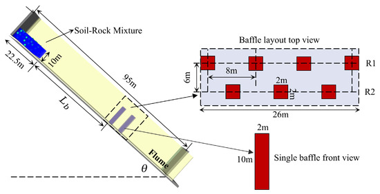
Figure 2.
Simplified model of the flume device.
Rock–soil mixture: The soil body is in length, width, and height, respectively. Boulders with a radius of are randomly embedded within the soil matrix. The motion of the soil is simulated by the MPM, while the boulders are modeled using the DEM. The MPM background grid has a uniform resolution of , with eight particles assigned per cell [52].
Baffle and structure system: Each baffle has a square cross-section with dimensions of and a height of . The baffles are arranged in a staggered configuration, with an inter-baffle spacing of and a row spacing of . The structure, which has a height of , is positioned at the end of the flume. Both the baffles and the structure are modeled using the SDEM and are assigned material properties corresponding to concrete. The influence of baffle positioning is analyzed by varying the distance between the boundary of the rock–soil mixture and the upstream edge of the baffle area.
Terrain: The terrain chute is also modeled using SDEM and is assigned the mechanical properties of rock. The influence of terrain slope is examined by varying the slope angle .
The physical and mechanical parameters employed for calculating the contact force are chosen based on representative values for natural materials reported in the literature [53]. These parameters were previously validated in the authors’ prior work. To maintain consistency, the same set of parameters is utilized in the current study, as summarized in Table 1.

Table 1.
Mechanical parameters used in the numerical simulations.
To quantitatively assess the protective effectiveness of the baffles, parametric studies are performed by varying the location of the baffles and the slope angle of the terrain. The simulation cases designed for these parametric analyses are outlined in Table 2.
Table 2.
Expanded numerical example summarization.
3.1. Impact Dynamics for Baffle’s Location
The interaction processes between the baffles and the soil–rock mixtures are briefly introduced to illustrate the changes in flow characteristics. Figure 3 presents snapshots illustrating the impact dynamics for different baffle locations. Despite the mixture flow arriving at the baffles at different times, the fundamental interaction processes across different cases remain similar. Similar processes can be found in previous studies [6,25,54].
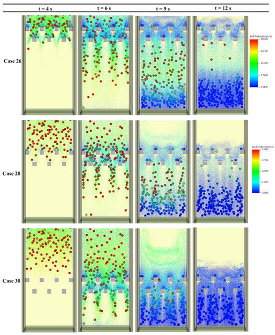
Figure 3.
Comparison of the dynamic flow processes at under different baffle configurations.
During the initial impact phase, the flow encounters the baffle array, resulting in the formation of prominent vertical jets behind the baffles. A substantial portion of the mixture passes through the gaps between them. The staggered configuration of the baffles plays a critical role in this interaction by significantly impeding the bulk movement of the flow. It is evident that the flow velocity is reduced after passing through the array, demonstrating the baffles’ effectiveness in dissipating the kinetic energy of the incoming flow.
As the impact continues, considerable splashing occurs within the baffle zone, leading to enhanced particle collisions. The flow interacts with both the first and second rows of baffles, causing pronounced disturbance and dispersion of the flow field. These effects result from the successive impacts and are further amplified as the granular jets, emerging from the gaps, are redirected and dispersed by the staggered elements of the second baffle row.
At the end of impact, the intensity of the interaction with the baffle array diminishes, marked by a notable reduction in particle splashing near the flow surface. No overflow is observed, as the baffle height is sufficient to prevent overtopping.
Figure 4 illustrates the evolution of the average flow velocity for both the soil and rock phases within the baffle area. In the early stages, the average velocity in Case 30 is notably higher than that of Case 26 and Case 28. This discrepancy is attributed to the location of the baffle array in Case 30 being further from the avalanche starting point. This longer distance allows the mixture to accelerate over a longer sliding path, thereby enabling a greater conversion of gravitational potential energy into kinetic energy before reaching the baffles.
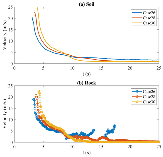
Figure 4.
Comparison of the average flow velocity for mixture flows under different baffle configurations. (a) is the soil part, (b) is the rock part.
3.2. Impact Dynamics for Slope Angle
Figure 5 presents snapshots illustrating the impact dynamics of the soil–rock mixture flow under varying slope angles, which exhibit similar patterns to the cases involving different baffle locations. From the perspective of energy, during the initial impact phase (t = 4 s), gravitational potential energy is converted into kinetic energy as the mixture accelerates down the slope. As the impact progresses (t = 6–9 s), the mixture flow collides with the baffle, leading to partial dissipation of kinetic energy through internal collisions among different flow components. Meanwhile, the boundary wall contributes significantly to energy dissipation by increasing frictional losses due to the confined flow conditions. By the end of the impact process (t = 12 s), the remaining mixture climbs the deposition ramp that forms in the dead zone behind the structure, converting its residual kinetic energy back into potential energy.
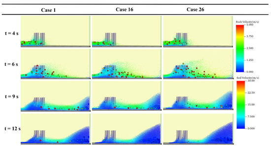
Figure 5.
Comparison of the dynamic flow processes at (m) with different slope angles.
As shown in Figure 6, the comparison reveals that the velocity differences among the various slope angle cases are relatively small. The influence of slope angle on velocity is less pronounced than that of the baffle location. In the rock velocity part, discontinuities can be observed, which are caused by the absence of rocks during those time intervals. While the soil velocity gradually decreases over time, the rock velocity exhibits noticeable fluctuations.
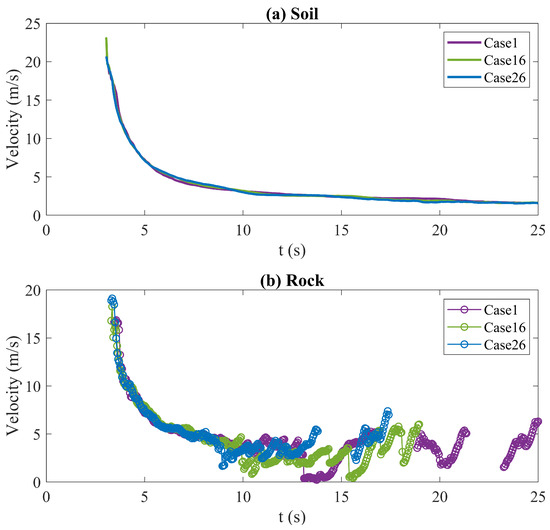
Figure 6.
Comparison of the average flow velocity for mixture flows with different slope angles. (a) is the soil part, (b) is the rock part.
4. Discussion
4.1. Effects of Baffle Position on Impact Forces Acting on Structures
Figure 7 illustrates the impact forces acting on the structure under different baffle locations. Although the tendency of the impact force acting on the structure does not exhibit significant variation across the different baffle positions, the magnitude of the impact force is directly related to the baffle location. A detailed examination of the force time histories shows a shift in magnitudes: prior to approximately 10 s, Case 26 exhibits the highest impact force and Case 30 the lowest. Subsequently, after this point, the force in Case 30 gradually increases to become the highest, whereas that in Case 26 decreases to the lowest level. This phenomenon is attributable to the different baffle positions, leading to different accumulation patterns. These changes in accumulation behavior directly influence the distribution and overall magnitude of the impact force on the structure.
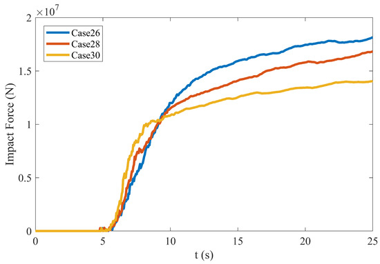
Figure 7.
Impact force acting on the structure as time progresses.
A sensitivity analysis was performed to quantify the influence of the sphero-radius parameter on impact forces. As shown in Figure 8, which presents the mean impact force and standard deviation from simulations with three different sphero-radii (0.1 m, 0.15 m and 0.2 m), the results demonstrate a clear sensitivity to this parameter. The significant standard deviation, illustrated by the error bars, indicates that larger sphero-radii consistently yield lower impact forces. This occurs because increasing the sphero-radius effectively enhances baffle roundness and the blockage profile of the baffle array, resulting in greater upstream retention of material and reduced transmitted loads on the downstream structure. These findings highlight that the sphero-radius not only contributes to numerical stability in contact detection but also directly influences the physical simulation outcomes, and therefore must be chosen carefully to represent the intended particle geometry.
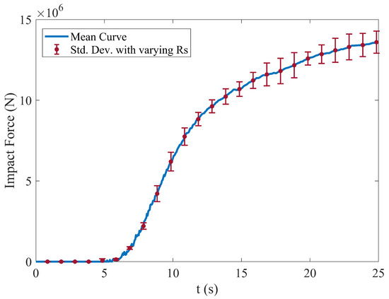
Figure 8.
Comparison of the impact force with different sphero-radius.
Compared with classical DEM, the principal advantage of SDEM is its ability to capture complex particle geometries with greater fidelity. The use of enveloping spheres in the spheropolygon formulation ensures more stable and robust contact force calculations, which allows the method to preserve both numerical stability and shape-dependent effects.
A series of simulations was conducted to evaluate the influence of the restitution coefficient on the predicted impact forces. The restitution coefficient is varied from 0.1 to 0.3. The results are summarized in Figure 9. The figure presents the mean impact force curve over time, with error bars indicating the standard deviation associated with the different restitution coefficients. The results indicate that the variation in impact forces is negligible, as the standard deviation remains very small throughout the impact event. This insensitivity can be attributed to the dense granular nature of the flow, where energy dissipation and momentum transfer are governed primarily by sustained frictional and multi-body contacts rather than by the energy loss associated with individual particle collisions.
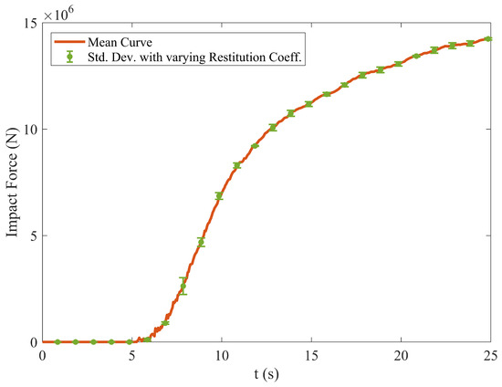
Figure 9.
Penetration depth with various velocities.
Figure 10 illustrates the accumulation patterns of the mixture flow at s behind the structure under different baffle location scenarios. Significant differences in the deposition profiles are observed among the three cases. In Cases 26 and 28, where the baffles are positioned relatively far from the structure, the mixture retains kinetic energy after passing through the baffle array, as indicated by the velocity contour plots. This continued flow leads to a larger volume of material accumulating behind the structure, resulting in a greater initial impact force compared to Case 30 (as shown in Figure 7). Conversely, in Case 30, the baffle’s close proximity to the structure causes the mixture to deposit almost immediately downstream of the baffle. Furthermore, the baffle itself bears a portion of the impact force, thereby reducing the initial load transmitted to the structure.
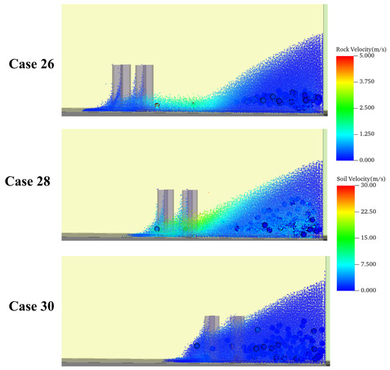
Figure 10.
Accumulation patterns of the mixture flow behind the structure.
4.2. Effects of Slope Angle on Impact Forces Acting on Structures
Figure 11 illustrates the influence of slope angle on the impact forces exerted by a soil–rock mixture flow on a structure. A direct relationship is evident: steeper slopes correspond to increased impact forces. This relationship is fundamentally rooted in energy conversion principles. A steeper slope provides the mixture with greater initial gravitational potential energy. As the mixture flows downhill under the influence of gravity, this potential energy is converted into kinetic energy. On steeper slopes, the mixture accelerates more rapidly and attains a higher velocity before impacting the structure. Since the impact force is directly related to the rate of change of momentum upon collision, the higher velocity, resulting from increased kinetic energy, produces a larger momentum change over a shorter duration, thereby generating a significantly greater impact force on the structure.
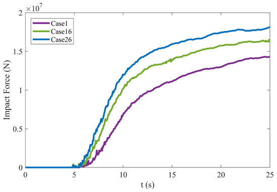
Figure 11.
Impact force acting on the structure with different slope angles.
Figure 12 shows the final accumulation patterns of the mixture as a function of slope angle. In Case 1, characterized by a gentler slope, the mixture possesses less initial potential energy. As a result, the sliding mass travels a shorter distance before dissipating its energy, causing it to stop and accumulate farther upstream from the structure. This leads to a relatively gentle accumulation profile. In contrast, Case 26 features a steeper slope, providing the mixture with greater kinetic energy. The arrival of this high energy flow is then restricted by the structure, limiting the available space for run-out and deposition. Consequently, incoming material stacks behind the structure, resulting in a steeper final accumulation profile.
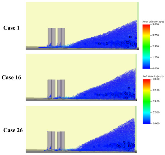
Figure 12.
Final accumulation patterns of the mixture behind the structure with different slope.
To improve the generality of our findings, we have reformulated the analysis in a dimensionless framework, ensuring that the results are scale-independent. The baffle placement is characterized by the dimensionless distance ratio, , where is the distance from the source and is the baffle height. Key output variables have also been normalized: the final static force is expressed relative to the initial gravitational weight of the soil mass, , and the kinetic energy is expressed relative to a characteristic potential energy, , where H and L are the initial height and length of the soil body, respectively. This dimensionless formulation allows the results to be readily extended and applied to different field scales and engineering configurations.
Figure 13 summarizes the final static forces for all cases. The results show a positive correlation between the final static force and the slope angle, indicating that steeper slopes generate greater static forces. Meanwhile, an inverse relationship is observed with respect to the baffle’s distance from the structure, increasing this distance leads to a reduction in the final static force. In practical applications, the slope angle of a natural hillside is often fixed, but the position of mitigation structures such as baffle arrays can be strategically engineered to effectively mitigate the destructive impact of debris flows on downstream infrastructure.
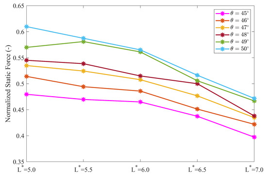
Figure 13.
Final static force with different cases.
4.3. Effects of Baffle Position on Impact Forces Acting on Baffle
Figure 14 presents the impact forces exerted on baffles positioned at different locations. As the baffle area comprises two rows of baffles, the impact forces on each row are calculated independently. To minimize boundary effects from the flume walls, the analysis focuses on the central baffle element in the first row.
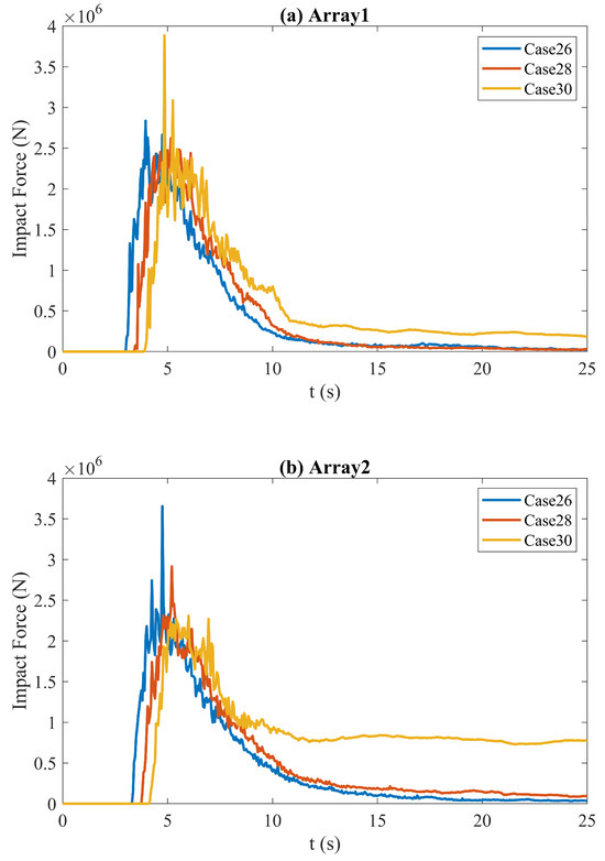
Figure 14.
Impact force acting on the baffle with different locations. (a) is Array 1, (b) is Array 2.
For the first row, Case 30 exhibits a distinct peak in impact force, which is attributed to direct rock collisions. When the influence of rock impact is excluded, the impact forces on the first-row baffles are generally similar across the different cases. In the second row, the impact forces are reduced relative to the first row, largely due to energy dissipation caused by the interaction between the mixture and the first-row baffles. Nonetheless, distinct peaks are still observed in the second-row force data, highlighting the complex and dynamic behavior of the soil–rock mixture flow.
4.4. Effects of Slopes Angle on Impact Forces Acting on Baffle
Figure 15 illustrates the influence of slope angle on the impact forces acting on the baffles. The general effect of slope angle is evident: as the angle increases, the corresponding impact force also rises. This trend is attributed to steeper slopes imparting greater kinetic energy to the mixture flow. However, an interesting deviation is noted in Case 1 (the gentlest slope) during the later phase of the impact, where it exhibits relatively higher impact forces compared to cases with steeper slopes. This phenomenon can be explained by the slower movement of the mixture in Case 1, resulting from the lower slope gradient. The reduced velocity allows for the gradual accumulation of a larger volume of material within the baffle zone over time, thereby contributing to increased impact forces during the later phase.
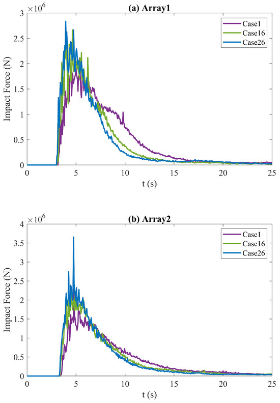
Figure 15.
Impact force acting on the baffle with different slope angles. (a) is Array 1, (b) is Array 2.
The timing and sequence of force peaks observed in the simulations have direct implications for structural performance. Repeated sharp force peaks, even when remaining below the ultimate strength of the baffles, may subject the structure to cyclic loading that can cause fatigue or progressive deterioration. In contrast, a single high-magnitude peak, typically associated with the direct impact of a large boulder, may exceed the material’s ultimate strength and result in brittle failure. In the present framework, baffles are modeled as rigid bodies within the DEM, which precludes explicit simulation of fracture. Future extensions of the model should therefore incorporate structural damage analyses, for example by coupling with Finite Element Method formulations, to enable evaluation of both immediate structural failure and long-term damage accumulation.
4.5. Effects of Baffle Position on Kinetic Energy
To further investigate the variation in kinetic energy of the soil–rock mixture flow, two monitoring zones were established relative to the baffle area: Monitoring Zone 1 (forward 5 m), positioned upstream of the baffle entrance, and Monitoring Zone 2 (backward 5 m), located downstream of its exit. The total kinetic energy of both the soil and rock components was calculated within these zones.
Figure 16 illustrates the total kinetic energy in these two monitoring zones as a function of baffle location. The kinetic energy within Monitoring Zone 1 increases with increasing . This trend is attributed to the longer distance the mixture travels downhill before reaching the baffle, allowing greater conversion of gravitational potential energy into kinetic energy. In contrast, the kinetic energy within Monitoring Zone 2 exhibits a decreasing trend with increasing (as the baffle is placed closer to the structure). This observation indicates that the baffle array effectively dissipates the kinetic energy of the mixture flow. The greater kinetic energy difference between the two zones can be observed in the figure when the baffle is located closer to the structure. This phenomenon is also consistent with the results presented in Figure 7, which show a reduction in impact force on the structure when the baffle is placed closer.
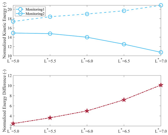
Figure 16.
Comparison of kinetic energy with different baffle location.
4.6. Effects of Slopes Angle on Kinetic Energy
Figure 17 illustrates the evolution of kinetic energy within the two monitoring zones under varying slope angles. In Monitoring Zone 1 and Monitoring Zone 2, kinetic energy increases proportionally with the slope angle. As shown in the subplot, the energy difference between the two zones widens with increasing slope angle. This growing disparity is attributed to the higher initial velocity and kinetic energy imparted to the mixture on steeper slopes. These conditions result in more energetic and intense collisions within the baffle region, leading to increased energy dissipation. Despite this enhanced dissipation, the kinetic energy in Monitoring Zone 2 continues to increase with slope angle. Therefore, steeper slopes yield greater kinetic energy downstream of the baffle, resulting in higher impact forces on the downstream structure. This conclusion is consistent with the findings in Figure 11, which demonstrate a positive correlation between slope steepness and structural impact.
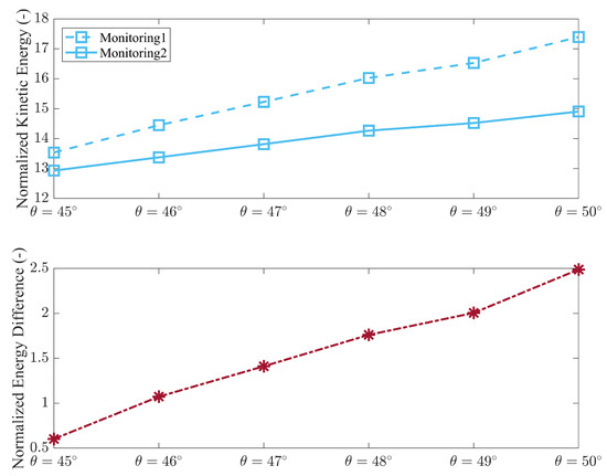
Figure 17.
Comparison of kinetic energy with different slope angles.
5. Conclusions
This research employed a sophisticated coupled MPM-DEM numerical framework to investigate the protective efficacy of baffle arrays against hazardous soil–rock mixture flows. This study specifically focused on the effects of baffle location and slope angle on the system’s protective efficacy. The key findings can be summarized as follows:
- Baffle arrays significantly influence the flow behavior of soil–rock mixture. When placed closer to the structure, baffles dissipate more kinetic energy and reduce the impact force on the structure. This is due to the shortened run-out distance and increased energy absorption by the baffles themselves. However, this configuration also increases the stress concentration on the baffles, necessitating a trade-off in design between structural protection and baffle durability.
- Increasing the slope angle leads to higher impact velocities and forces due to the greater conversion of gravitational potential energy into kinetic energy. Steeper slopes cause more concentrated impact zones and sharper accumulation gradients, intensifying the structural demands on both the baffle and downstream infrastructure.
- By monitoring kinetic energy upstream and downstream of the baffle array, it was observed that energy loss through baffle interaction increases as the baffles are placed closer to the structure. This indicates a more efficient dissipation mechanism, but also implies greater mechanical demands on the baffle components, especially under high-slope conditions.
In summary, the MPM-DEM coupled method proved effective in analyzing the complex dynamics of soil–rock mixture flows and their interaction with protective structures. Our results suggest that a normalized baffle distance of provides an effective way to mitigate downstream impact forces, providing valuable insights for the design and optimization of landslide and debris flow mitigation systems.
In conclusion, while the present study provides new insights into the interaction between soil–rock mixture flows and baffle arrays, several limitations remain. The numerical experiments were conducted within an idealized flume geometry, and extending the analysis to more complex topographies and alternative baffle configurations could further optimize protective designs. However, the absence of water in the current framework overlooks an important factor in real debris flows, integrating fluid dynamics through coupled two-phase flow models represents a critical step for future studies. Finally, addressing scale effects, parameter uncertainties, and the structural response of baffles themselves would help bridge the gap between numerical predictions and practical engineering applications.
Author Contributions
Conceptualization, H.Z., S.R., and P.Z.; methodology, H.Z., S.R., Z.S., X.T., and P.Z.; software, S.R. and P.Z.; validation, H.Z., Z.S., C.F., and R.L.; formal analysis, H.Z., S.R., and Z.S.; investigation, H.Z., S.R., and Z.S.; resources, Z.S., C.F., and R.L.; writing—original draft preparation, H.Z. and S.R.; writing—review and editing, X.T. and P.Z.; visualization, H.Z., Z.S., C.F., and R.L.; supervision, S.R. and P.Z.; project administration, S.R., X.T., and P.Z.; funding acquisition, S.R., X.T., and P.Z. All authors have read and agreed to the published version of the manuscript.
Funding
This research was funded by the Scientific Research Starting Fund from Hangzhou Dianzi University (No. KYS015624320), the Key Project of Westlake Institute for Optoelectronics (Grant No. 2023GD001), the Fund from Hangzhou Dianzi University (No. KYH043125034), and the Fund from China Aluminum International Engineering Co., Ltd. (No. ZC-06-202407-020), Zhejiang Province Leading Goose Plan Project (No. 2025C02017).
Institutional Review Board Statement
Not applicable.
Informed Consent Statement
Not applicable.
Data Availability Statement
All data generated or analyzed during this research are included in this paper.
Acknowledgments
The presented simulations were conducted based on the ComFluSoM open-source library (https://github.com/peizhang-cn/ComFluSoM, accessed on 13 August 2025).
Conflicts of Interest
Author Zhongyue Shen was employed by the company Zhejiang Yunce Land Planning and Design Co., Ltd. and authors Can Fu and Rong Lan were employed by the company Kunming Engineering & Research Institute of Nonferrous Metallurgy Co., Ltd. The remaining authors declare that the research was conducted in the absence of any commercial or financial relationships that could be construed as a potential conflict of interest.
References
- Pradeep, S.; Arratia, P.E.; Jerolmack, D.J. Origins of complexity in the rheology of Soft Earth suspensions. Nat. Commun. 2024, 15, 7432. [Google Scholar] [PubMed]
- Cui, K.F.; Zhou, G.G.; Man, T.; Huang, Y.; Zhang, Y.; Lu, X.; Zhao, T. Modeling the dense granular flow rheology of particles with different surface friction: Implications for geophysical mass flows. J. Geophys. Res. Earth Surf. 2025, 130, e2024JF008048. [Google Scholar] [CrossRef]
- Ma, Z.; Mei, G. Deep learning for geological hazards analysis: Data, models, applications, and opportunities. Earth-Sci. Rev. 2021, 223, 103858. [Google Scholar]
- Iverson, R.M. The physics of debris flows. Rev. Geophys. 1997, 35, 245–296. [Google Scholar] [CrossRef]
- Liu, C.; Yu, Z.; Zhao, S. A coupled SPH-DEM-FEM model for fluid-particle-structure interaction and a case study of Wenjia gully debris flow impact estimation. Landslides 2021, 18, 2403–2425. [Google Scholar] [CrossRef]
- Ng, C.W.W.; Jia, Z.; Poudyal, S.; Bhatta, A.; Liu, H. Two-phase MPM modelling of debris flow impact against dual rigid barriers. Géotechnique 2023, 74, 1390–1403. [Google Scholar] [CrossRef]
- Goodwin, S.R.; Choi, C.E.; Yune, C.Y. Towards rational use of baffle arrays on sloped and horizontal terrain for filtering boulders. Can. Geotech. J. 2021, 58, 1571–1589. [Google Scholar] [CrossRef]
- Du, J.; Chang, D.; Lee, C.; Su, Y.; Choi, C.E.; Zhang, J. Mitigation of rockfall geohazards: Full-scale investigation of the performance of a practical baffle design for direct use in the field. Eng. Geol. 2024, 337, 107586. [Google Scholar] [CrossRef]
- Zhou, G.G.; Hu, H.; Song, D.; Zhao, T.; Chen, X. Experimental study on the regulation function of slit dam against debris flows. Landslides 2019, 16, 75–90. [Google Scholar] [CrossRef]
- Yang, H.; Haque, E.; Song, K. Experimental study on the effects of physical conditions on the interaction between debris flow and baffles. Phys. Fluids 2021, 33, 056601. [Google Scholar] [CrossRef]
- Kim, B.J.; Yune, C.Y. Flume investigation of debris flow entrained boulders with cylindrical baffles and a rigid barrier. Eng. Geol. 2025, 344, 107836. [Google Scholar] [CrossRef]
- Ng, C.W.W.; Choi, C.; Song, D.; Kwan, J.; Koo, R.; Shiu, H.; Ho, K. Physical modeling of baffles influence on landslide debris mobility. Landslides 2015, 12, 1–18. [Google Scholar] [CrossRef]
- Bi, Y.Z.; Wang, D.P.; Yan, S.X.; Li, Q.Z.; He, S.M. Research on the blocking effect of baffle-net structure on rock avalanches: Consider the influence of particle splashing. Bull. Eng. Geol. Environ. 2023, 82, 277. [Google Scholar] [CrossRef]
- Kim, B.J.; Yune, C.Y. Flume investigation of cylindrical baffles on landslide debris energy dissipation. Landslides 2022, 19, 3043–3060. [Google Scholar] [CrossRef]
- Man, T.; Huppert, H.E.; Galindo-Torres, S.A. Run-out scaling of granular column collapses on inclined planes. J. Fluid Mech. 2025, 1002, A50. [Google Scholar] [CrossRef]
- Huang, Y.; Zhang, B.; Zhu, C. Computational assessment of baffle performance against rapid granular flows. Landslides 2021, 18, 485–501. [Google Scholar] [CrossRef]
- Marveggio, P.; Zerbi, M.; Redaelli, I.; di Prisco, C. Granular material regime transitions during high energy impacts of dry flowing masses: MPM simulations with a multi-regime constitutive model. Int. J. Numer. Anal. Methods Geomech. 2024, 48, 3699–3724. [Google Scholar] [CrossRef]
- Gong, S.; Zhao, T.; Zhao, J.; Dai, F.; Zhou, G.G. Discrete element analysis of dry granular flow impact on slit dams. Landslides 2021, 18, 1143–1152. [Google Scholar] [CrossRef]
- Ozbay, A.; Cabalar, A. FEM and LEM stability analyses of the fatal landslides at Çöllolar open-cast lignite mine in Elbistan, Turkey. Landslides 2015, 12, 155–163. [Google Scholar] [CrossRef]
- Soga, K.; Alonso, E.; Yerro, A.; Kumar, K.; Bandara, S. Trends in large-deformation analysis of landslide mass movements with particular emphasis on the material point method. Géotechnique 2016, 66, 248–273. [Google Scholar] [CrossRef]
- Carbonell, J.M.; Monforte, L.; Ciantia, M.O.; Arroyo, M.; Gens, A. Geotechnical particle finite element method for modeling of soil-structure interaction under large deformation conditions. J. Rock Mech. Geotech. Eng. 2022, 14, 967–983. [Google Scholar] [CrossRef]
- Zhang, X.; Krabbenhoft, K.; Sheng, D.; Li, W. Numerical simulation of a flow-like landslide using the particle finite element method. Comput. Mech. 2015, 55, 167–177. [Google Scholar] [CrossRef]
- Peng, C.; Li, S.; Wu, W.; An, H.; Chen, X.; Ouyang, C.; Tang, H. On three-dimensional SPH modelling of large-scale landslides. Can. Geotech. J. 2022, 59, 24–39. [Google Scholar]
- Bui, H.H.; Nguyen, G.D. Smoothed particle hydrodynamics (SPH) and its applications in geomechanics: From solid fracture to granular behaviour and multiphase flows in porous media. Comput. Geotech. 2021, 138, 104315. [Google Scholar] [CrossRef]
- Yang, E.; Bui, H.H.; Nguyen, G.D.; Choi, C.E.; Ng, C.W.; De Sterck, H.; Bouazza, A. Numerical investigation of the mechanism of granular flow impact on rigid control structures. Acta Geotech. 2021, 16, 2505–2527. [Google Scholar] [CrossRef]
- Ren, S.; Zhang, P.; Zhao, Y.; Tian, X.; Galindo-Torres, S. A coupled metaball discrete element material point method for fluid–particle interactions with free surface flows and irregular shape particles. Comput. Methods Appl. Mech. Eng. 2023, 417, 116440. [Google Scholar] [CrossRef]
- Pan, S.; Nomura, R.; Ling, G.; Takase, S.; Moriguchi, S.; Terada, K. Variable passing method for combining 3D MPM–FEM hybrid and 2D shallow water simulations of landslide-induced tsunamis. Int. J. Numer. Methods Fluids 2024, 96, 17–43. [Google Scholar] [CrossRef]
- Li, X.; Yan, Q.; Zhao, S.; Luo, Y.; Wu, Y.; Wang, D. Investigation of influence of baffles on landslide debris mobility by 3D material point method. Landslides 2020, 17, 1129–1143. [Google Scholar] [CrossRef]
- Hu, Y.; Zhu, Y.; Li, H.; Li, C.; Zhou, J. Numerical estimation of landslide-generated waves at Kaiding Slopes, Houziyan Reservoir, China, using a coupled DEM-SPH method. Landslides 2021, 18, 3435–3448. [Google Scholar]
- Bi, Y.; Huang, Y.; Zhang, B.; Pu, J. CFD-DEM numerical investigation of the effects of water content and inclination angle on interactions between debris flows and slit dam. Comput. Geotech. 2024, 170, 106273. [Google Scholar] [CrossRef]
- Peng, C.; Zhan, L.; Wu, W.; Zhang, B. A fully resolved SPH-DEM method for heterogeneous suspensions with arbitrary particle shape. Powder Technol. 2021, 387, 509–526. [Google Scholar] [CrossRef]
- Jiang, Y.; Zhao, Y.; Choi, C.E.; Choo, J. Hybrid continuum–discrete simulation of granular impact dynamics. Acta Geotech. 2022, 17, 5597–5612. [Google Scholar] [CrossRef]
- Liang, W.; Zhao, J.; Wu, H.; Soga, K. Multiscale modeling of anchor pullout in sand. J. Geotech. Geoenviron. Eng. 2021, 147, 04021091. [Google Scholar] [CrossRef]
- Liang, W.; Zhao, S.; Wu, H.; Zhao, J. Bearing capacity and failure of footing on anisotropic soil: A multiscale perspective. Comput. Geotech. 2021, 137, 104279. [Google Scholar] [CrossRef]
- Ren, S.; Zhang, P.; Man, T.; Galindo-Torres, S. Numerical assessments of the influences of soil–boulder mixed flow impact on downstream facilities. Comput. Geotech. 2023, 153, 105055. [Google Scholar] [CrossRef]
- Li, J.; Wang, B.; Zhang, J.; Zhang, X. Investigation of the protective effect of baffles against soil-rock mixture disasters using the MPM-DEM method. Comput. Geotech. 2025, 180, 107107. [Google Scholar] [CrossRef]
- Gogolik, S.; Kopras, M.; Szymczak-Graczyk, A.; Tschuschke, W. Experimental evaluation of the size and distribution of lateral pressure on the walls of the excavation support. J. Build. Eng. 2023, 73, 106831. [Google Scholar] [CrossRef]
- Kopras, M.; Buczkowski, W.; Szymczak-Graczyk, A.; Walczak, Z.; Gogolik, S. Experimental validation of deflections of temporary excavation support plates with the use of 3D modelling. Materials 2022, 15, 4856. [Google Scholar] [CrossRef]
- Zhang, X.; Chen, Z.; Liu, Y. The Material Point Method: A Continuum-Based Particle Method for Extreme Loading Cases; Academic Press: New York, NY, USA, 2016. [Google Scholar]
- Ren, S.; Liu, Z.; Trujillo-Vela, M.; Galindo-Torres, S.; Tian, X.; Zhang, P. Simulation of solitary wave generation and wave-structure interactions using an MPM-SDEM coupling scheme. Ocean. Eng. 2025, 340, 122195. [Google Scholar] [CrossRef]
- Bardenhagen, S.; Brackbill, J.; Sulsky, D. The material-point method for granular materials. Comput. Methods Appl. Mech. Eng. 2000, 187, 529–541. [Google Scholar] [CrossRef]
- Shi, Y.; Guo, N.; Yang, Z. GeoTaichi: A Taichi-powered high-performance numerical simulator for multiscale geophysical problems. Comput. Phys. Commun. 2024, 301, 109219. [Google Scholar] [CrossRef]
- Clausen, J.; Damkilde, L.; Andersen, L.V. Robust and efficient handling of yield surface discontinuities in elasto-plastic finite element calculations. Eng. Comput. 2015, 32, 1722–1752. [Google Scholar] [CrossRef]
- Galindo-Torres, S.; Pedroso, D. Molecular dynamics simulations of complex-shaped particles using Voronoi-based spheropolyhedra. Phys. Rev. E—Stat. Nonlinear Soft Matter Phys. 2010, 81, 061303. [Google Scholar]
- Zhang, X.; Huang, T.; Ge, Z.; Man, T.; Huppert, H.E. Infiltration characteristics of slurries in porous media based on the coupled Lattice-Boltzmann discrete element method. Comput. Geotech. 2025, 177, 106865. [Google Scholar]
- Zhang, P.; Qiu, L.; Chen, Y.; Zhao, Y.; Kong, L.; Scheuermann, A.; Li, L.; Galindo-Torres, S.A. Coupled metaball discrete element lattice Boltzmann method for fluid-particle systems with non-spherical particle shapes: A sharp interface coupling scheme. J. Comput. Phys. 2023, 479, 112005. [Google Scholar] [CrossRef]
- Zhang, P.; Dong, Y.; Galindo-Torres, S.; Scheuermann, A.; Li, L. Metaball based discrete element method for general shaped particles with round features. Comput. Mech. 2021, 67, 1243–1254. [Google Scholar] [CrossRef]
- Luding, S. Introduction to discrete element methods: Basic of contact force models and how to perform the micro-macro transition to continuum theory. Eur. J. Environ. Civ. Eng. 2008, 12, 785–826. [Google Scholar] [CrossRef]
- Ren, S.; Zhang, P.; Galindo-Torres, S. A coupled discrete element material point method for fluid–solid–particle interactions with large deformations. Comput. Methods Appl. Mech. Eng. 2022, 395, 115023. [Google Scholar] [CrossRef]
- Moriguchi, S.; Borja, R.I.; Yashima, A.; Sawada, K. Estimating the impact force generated by granular flow on a rigid obstruction. Acta Geotech. 2009, 4, 57–71. [Google Scholar] [CrossRef]
- Ciamarra, M.P.; Lara, A.H.; Lee, A.T.; Goldman, D.I.; Vishik, I.; Swinney, H.L. Dynamics of drag and force distributions for projectile impact in a granular medium. Phys. Rev. Lett. 2004, 92, 194301. [Google Scholar] [CrossRef] [PubMed]
- Bardenhagen, S.G.; Kober, E.M. The generalized interpolation material point method. Comput. Model. Eng. Sci. 2004, 5, 477–496. [Google Scholar]
- Terzaghi, K.; Peck, R.B.; Mesri, G. Soil Mechanics in Engineering Practice; John Wiley & Sons: Hoboken, NJ, USA, 1996. [Google Scholar]
- Luo, H.; Zhang, L.; He, J.; Zhou, J. Performance of debris flow barriers: An energy perspective. Acta Geotech. 2025, 20, 987–1000. [Google Scholar] [CrossRef]
Disclaimer/Publisher’s Note: The statements, opinions and data contained in all publications are solely those of the individual author(s) and contributor(s) and not of MDPI and/or the editor(s). MDPI and/or the editor(s) disclaim responsibility for any injury to people or property resulting from any ideas, methods, instructions or products referred to in the content. |
© 2025 by the authors. Licensee MDPI, Basel, Switzerland. This article is an open access article distributed under the terms and conditions of the Creative Commons Attribution (CC BY) license (https://creativecommons.org/licenses/by/4.0/).