1. Introduction
Digital twin technology creates high-fidelity models of physical entities through digital methods, mapping information such as their attributes, behaviors, states, and performance to a virtual space [
1]. By leveraging data fusion, data analysis, and decision optimization, it enables real-time analysis, simulation, and prediction of the performance and operational status of these physical entities [
2]. This technology allows for continuous monitoring throughout the full service life cycle of a crane, enhancing control over equipment operational status. It thus provides a scientific foundation for fault prediction, maintenance decision-making, and performance optimization. In terms of numerical simulation research, scholars both domestically and internationally have achieved remarkable results, but several technical bottlenecks remain. Although the Component Mode Synthesis order reduction method developed by Moi et al. reduced the state assessment time to less than 50 ms, its fixed parameter characteristics make it difficult to adapt to the evolution of structural damage, resulting in a gradual decrease in assessment accuracy over time [
3,
4]. The Gaussian process surrogate model designed by He Xiwang et al. achieves 85% prediction accuracy with only 50 sets of training data, but experiences a response delay of 0.5–1 s when facing sudden load changes [
5]. The physics-informed neural network proposed by Fu Ling et al. performs well in predicting fatigue damage in boom systems, but the prediction error increases significantly when the data volume is insufficient [
6]. Wang et al. constructed a real-time simulation model based on the Krylov subspace reduction method, which greatly improved computational efficiency but had limited adaptability to nonlinear operating conditions [
7]. Lai et al. developed a shape-integrated digital twin modeling method that achieved stress analysis verification, but the computational complexity introduced by the integration of multiple models limited the system’s real-time performance [
8].
In the field of structural performance assessment, existing research faces many challenges. The SVM load assessment model developed by Mudasir et al. [
9], the ANSYS main beam strength analysis by Lin et al. [
10], the deflection curve structural stiffness assessment method proposed by Anatoliy et al. [
11], the nominal stress method by Chen Li et al. [
12], and the hot spot stress method for fatigue life assessment by Li Yongliang et al. are all limited to the independent analysis of a single performance indicator [
13]. Yan Bo et al. developed the FAHP safety evaluation system, and Zheng et al. proposed a fault tree–Bayesian network diagnostic framework, which achieves multi-indicator comprehensive evaluation but remains confined to offline analysis [
14,
15]. The physics-informed neural networks developed by Chen et al. showed good fatigue life prediction capabilities, but they are difficult to adapt to dynamically changing working conditions [
16]. The digital twin fatigue prediction system developed by Schmid et al. relies on a large amount of simulation data, and its real-time performance needs improvement [
17]. Although the fault tree–Bayesian network integration method developed by Feng et al. overcomes the limitations of traditional FTA, the complex calculation process hinders its application in real-time monitoring [
18]. While these research results have made significant progress, there are still clear deficiencies in real-time response capabilities, multi-indicator collaborative evaluation, and dynamic adaptability. More efficient numerical calculation methods and more intelligent comprehensive evaluation systems need to be developed.
In response to the above technical bottlenecks, this research proposes an innovative solution: first, a BO-LightGBM-based surrogate model is developed to automatically tune parameters through Bayesian optimization algorithms, thereby improving prediction accuracy while ensuring computational efficiency; second, a multi-indicator fusion digital twin evaluation system is constructed, integrating finite element analysis, surrogate models, and real-time monitoring technologies to establish a comprehensive evaluation system covering multiple dimensions, such as stress, deformation, and fatigue life.
2. Finite Element Analysis of Telescopic Cranes
2.1. Stress Analysis of Telescopic Cranes and Database Establishment
The real-time boom length of the telescopic boom is
. When the boom angle
is 0°, the maximum working radius of the front
section of the boom is
. Let the telescopic length of each section of the boom be
. When
, only two sections of the boom are telescoped, and the telescopic length is
. Similarly, the telescopic length of each section of the boom is
, as shown in
Table 1.
From
Table 1, we can see that the real-time boom length can be divided into three ranges according to the drive section boom, namely
,
, and
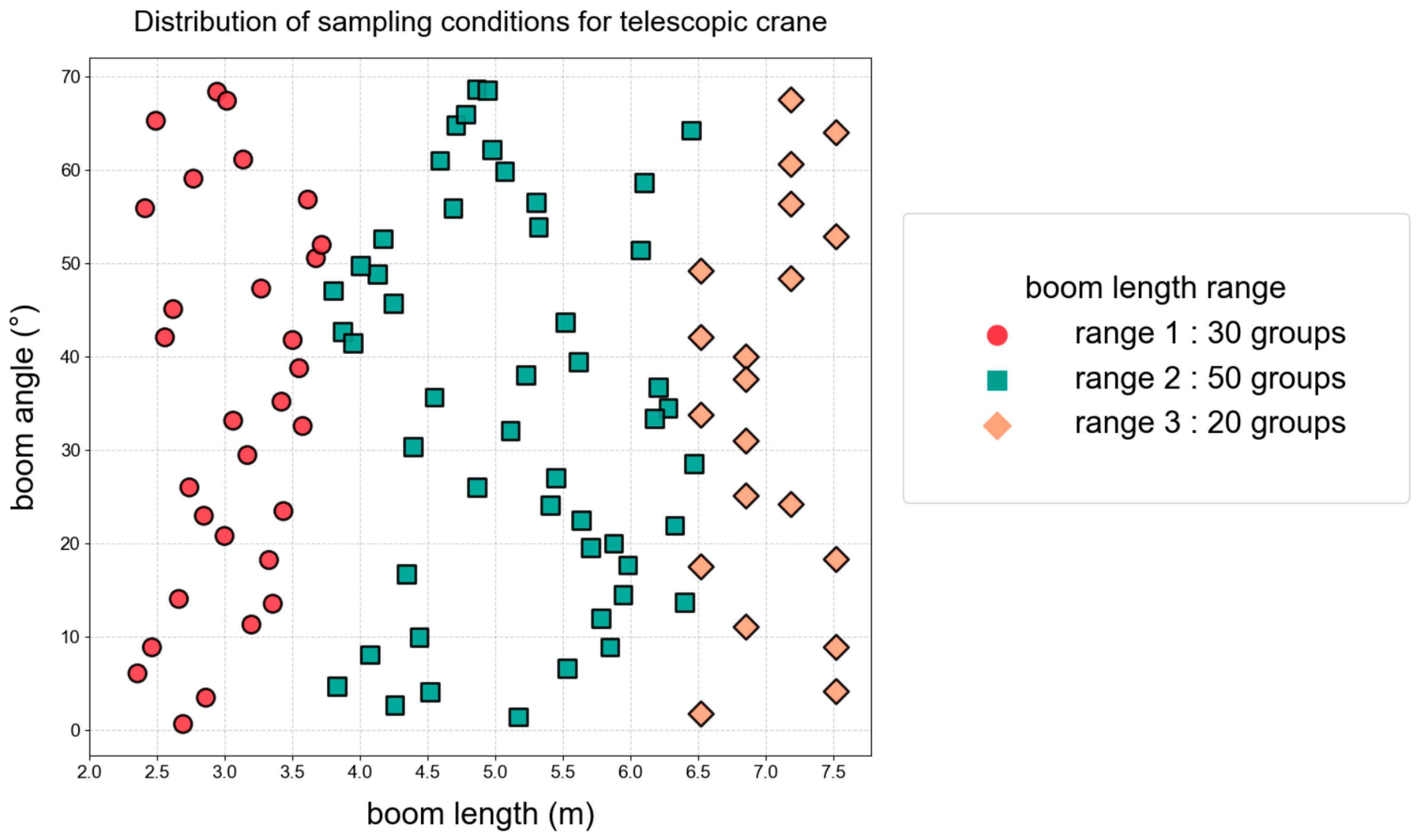
. To ensure the reasonable distribution of sample points in actual use scenarios, stratified Latin hypercube sampling (LHS) was used to generate 30, 50, and 20 sets of operating condition samples in the three ranges, respectively, for a total of 100 sets. Finally, the boom angle and real-time boom length (
) were sampled using the LHS method, and the sampling results are shown in
Figure 1.
For the 100 sample working conditions, structural stress distribution data under different combinations of boom length and boom angle were obtained through finite element numerical simulations. These data were then used for the subsequent training of the surrogate model.
2.2. Finite Element Modeling and Boundary Condition Setup
Using SOLIDWORKS 2022, a 3D model of the telescopic boom and its saddle was created based on the CAD drawings provided in the manual for the Mighty Crane Model CR235GL (R&B ENGINEERING CO.,LTD., Tokyo, Japan).Model preprocessing, material parameter configuration, material model selection, meshing, and boundary condition setup were carried out in ANSYS Workbench (version 2022 R2). Finite element models were established and analyzed for 100 sets of sample operating conditions.
The boom of the telescopic arm is fabricated from Q235 steel plates welded together. Each boom section is connected via sliding blocks made of Q215 material, while other critical structural components are made of Q460 material. Material parameters are sourced from the GB/T 700-2006 standard (carbon structural steel) and the GB/T 1591-2008 standard (low-alloy high-strength structural steel) [
19,
20]. Specific parameters are detailed in the
Table 2.
The telescopic arm and saddle are plate–shell structures, meshed using the SHELL281 shell element. The slider structure utilizes the SOLID187 solid element, and its node connection sequence is exported for constructing the cloud diagram on the digital twin platform.
Refer to the crane design standard GB/T 3811-2008 to calculate the loads on the telescopic crane [
21], including self-weight, rated lifting load, hoisting wire rope tension, and hoisting lateral force. Set the boundary conditions as shown in
Figure 2, with the gravity direction along the—Y axis. To prevent excessive local structural stiffness, apply remote displacement to the saddle base surface and impose full constraints to restrict rigid-body motion, allowing elastic deformation in local shell elements. A cylindrical pair is applied between the boom cylinder and its piston, constraining displacement along the piston’s extension/retraction direction (local Z-axis). A compression-only constraint is applied at the end bearing of the first boom section to simulate the cylindrical surface constraints from pins and bolts, matching its loading conditions. Load mass is applied via mass points. Since the mass points do not exceed the rated load and do not induce plastic deformation, a linear elastic material model is selected.
2.3. Finite Element Analysis of Fatigue Life
According to GB/T 3811-2008, the target telescopic crane has a usage class of , a load condition class of , and a working class of . Based on the equipment manual and systematic operation logs of the target telescopic crane, the average operational cycle frequency is statistically calculated to be 10 cycles per hour. Under conventional operating conditions, assuming an 8 h daily work period and 200 rated working days per year, the annual operational cycle for this equipment totals 16,000 cycles. The fatigue life was evaluated for the extreme lifting conditions as an operational cycle, with the boom angle changing from 0° to 45° in 5 s, maintained for 5 s, and finally returning from 45° to 0° in the last 5 s.
ANSYS Workbench was used to modify the finite element model and establish a multi-time-step finite element model based on the extreme operational cycle. A multi-time-step Z-direction displacement constraint was then applied to the cylindrical pair between the slewing cylinder and the slewing cylinder piston.
The multi-time-step finite element model was imported into ANSYS nCode DesignLife for fatigue life analysis, and the displacement time steps are summarized in
Table 3.
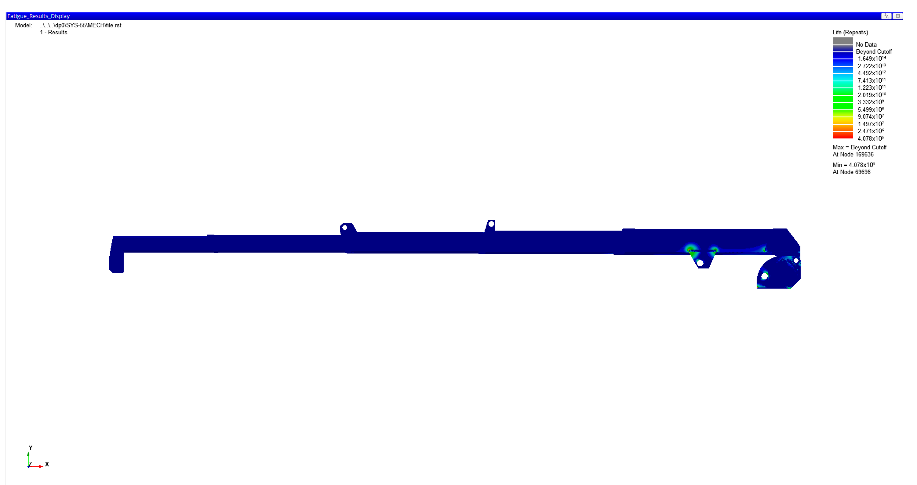
The fatigue life contour map of the telescopic arm is shown in
Figure 3. The weakest part of the structure is the connection between the side ribs and one section of the arm. The fatigue life is 4.078 × 10
5 stress cycles. Based on actual working conditions, with 16,000 operational cycles per year, the target telescopic crane service life can reach 25.49 years.
2.4. Data Preprocessing
In the structural analysis of telescopic cranes, due to differences in the rated loads corresponding to different working radii, it is difficult to directly sample the applied loads randomly. Given that the relationship between applied load and stress typically follows the linear elasticity assumption and small deformation assumption when the applied load remains within the yield material strength range, an increase in load mass exhibits a linear relationship with stress variation at finite element nodes within this applied load range. Through finite element analysis, we found that within this applied load range, the variation in node stress with increasing load mass follows a linear trend. Based on this, this study employs a linear conversion method to simplify the calculation process, ensuring sufficient analytical accuracy while maintaining computational efficiency. When the initial load is 0 kg, the finite element node stress is
, and when the load is 1 kg, the stress is
. Then, the node stress
when the load is
can be determined by the following linear relationship:
(1) In the above formula, k is the stress load coefficient, which represents the amount of stress change caused by a unit mass. To determine this coefficient, two extreme working conditions were selected for finite element analysis in this research: working condition 1 applies only the self-weight of the lifting device system ( = 0 kg), and working condition 2 applies both the self-weight of the lifting device system and a load of 1 kg ( = 1 kg). After calculating the stress load coefficient using Formulas (1) and (2) can be used to quickly convert the structural stress under different load masses.
This research employs a multi-scale feature fusion method to process the data. The core processing flow is as follows: the node coordinates
are used as local scale inputs to represent the geometric position of each node;
and
are used as global feature inputs, which are combined with the local features of each node through a broadcast mechanism to form a comprehensive feature vector. The overall structure of the algorithm used in this research is shown in Equation (3). The algorithm inputs are the coordinates of each finite element node
, the extension length of each arm
, and the boom angle
. The algorithm outputs a list of stresses for all nodes
.
3. Establishment of Stress Surrogate Model
3.1. LightGBM Algorithm
In engineering practice, surrogate models have become an effective alternative to complex system calculations, and various typical modeling methods have been developed. Polynomial regression models are known for their simple mathematical expressions and highly interpretable parameters [
22]. Neural network models perform well in complex system modeling due to their deep non-linear mapping capabilities [
23]. Support vector regression effectively handles high-dimensional feature space problems through kernel function transformations [
24]. Gradient boosting regression adopts an ensemble learning paradigm to construct robust prediction models by iteratively optimizing weak predictors [
25].
In constructing the stress surrogate model for the telescopic crane, this study comprehensively evaluated the applicability of various modeling methods and their engineering feasibility. Ultimately, the gradient boosting regression algorithm was selected over traditional approaches such as polynomial regression, neural networks, and support vector regression. This decision was grounded in the unique data scale and task requirements of this research, with the rationale primarily reflected in the following three aspects:
Gradient Boosting Regression demonstrates exceptional generalization capability under small sample conditions. This study conducted modeling based solely on 100 finite element samples combining different boom lengths and boom angles. Traditional deep neural networks are prone to overfitting due to excessive parameters, yielding low loss function values on the training set but significantly lacking in extrapolation prediction reliability. Polynomial regression, while structurally simple, has limited capability in capturing highly nonlinear relationships and lacks robustness in degree selection. Gradient Boosting Regression (GBR) integrates multiple weak learners (decision trees) and incorporates mechanisms such as tree structure constraints and leaf node output regularization. This approach extracts robust features from limited samples, balancing model complexity control with fitting accuracy, thereby significantly enhancing the model’s prediction stability and accuracy under unknown operating conditions.
Gradient Boosting Regression demonstrates robust representation capabilities for complex nonlinear mapping relationships. Crane node stress exhibits strong nonlinearity and high coupling characteristics with respect to boom length and boom angle variations, making explicit mathematical expressions challenging to formulate. Gradient Boosting Regression employs a forward stepwise algorithm to progressively fit residuals, enabling adaptive capture of complex interactions between variables. Without relying on manually predefined kernel functions (as in Support Vector Regression), it achieves accurate modeling of the underlying physical mechanisms between inputs and outputs, thereby reconstructing node stress distributions with greater precision.
The Gradient Boosting Regression algorithm offers significant computational efficiency advantages when handling high-dimensional output tasks. This study requires simultaneous prediction of stress values for tens of thousands of finite element nodes, representing a typical high-dimensional output regression problem. Traditional methods like Support Vector Regression would necessitate building independent regression models for each node, incurring substantial computational overhead. Gradient Boosting Regression, with its fast training speed and low memory consumption, supports efficient batch modeling, making independent regression training for each node a viable strategy.
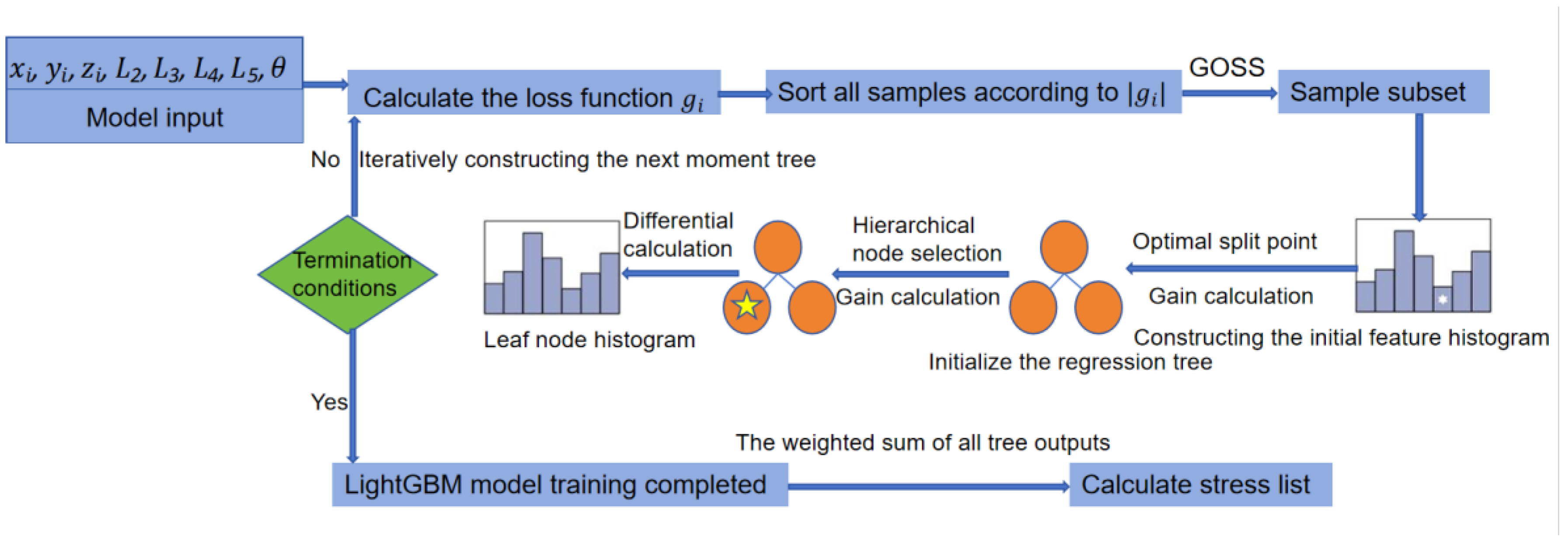
Building upon the traditional Gradient Boosted Decision Trees (GBDTs) architecture, this study selected the LightGBM algorithm as the core modeling framework [
26]. The implementation workflow of the LightGBM algorithm is illustrated in
Figure 4. Model training strictly follows LightGBM’s standard workflow, including feature preprocessing, gradient-based one-sided sampling, histogram generation and split point search, hierarchical node splitting, and histogram differential optimization. Through iterative construction of regression trees, the final prediction output is formed via weighted accumulation. To validate LightGBM’s effectiveness in this study, we subsequently conducted comparative experiments between LightGBM and XGBoost, evaluating their performance in prediction accuracy, computational efficiency, and training time.
3.2. Five-Fold Cross-Validation
To improve the generalization ability of the surrogate model on a limited dataset and reduce the risk of overfitting, this research employs k-fold cross-validation to train and evaluate the surrogate model [
27]. The training set is randomly divided into k mutually exclusive subsets. In each iteration, k − 1 of the data is used as the training set, and the remaining 1 is used as the validation set. After repeating k times, the mean absolute error (MAE) is taken as the evaluation result.
Based on the characteristics of the telescopic boom movement mechanism, a hierarchical sampling mechanism is established. Using the boom length parameters as hierarchical variables, which are consistent with the LHS sampling ratio used to construct the simulation stress database, the database is divided into three sub-databases. This ensures that each fold adheres to the real-time boom length distribution ratio of 3:5:2. Through hierarchical five-fold cross-validation, it is guaranteed that each training and validation subset corresponds to the overall boom length distribution.
Based on the characteristics of hierarchical five-fold cross-validation, this study eliminates the need for manual division of the validation set. Using the boom length parameter as the stratification variable, the dataset is divided into a training set and a test set in a 4:1 ratio, effectively avoiding model overfitting caused by parameter distribution bias. The training set undergoes hyperparameter optimization through five-fold cross-validation and the Bayesian optimization (BO) algorithm, while the test set remains isolated throughout the entire process to prevent any data leakage. It serves as the final benchmark for evaluating the model’s generalization ability, assessing its predictive performance on unseen data.
3.3. Hyperparameter Optimization for BO-XGBoost and BO-LightGBM
When performing hyperparameter optimization for BO-XGBoost using Optuna (version 4.2.1), the objective function was set to minimize the average value achieved through five-fold cross-validation [
28]. Seven hyperparameters, including the learning rate and maximum tree depth, were optimized. Logarithmic scale sampling was applied to the learning rate, while uniform integer sampling was used for parameters such as maximum tree depth and the number of leaves. Uniform continuous sampling was employed for the remaining hyperparameters. Specific settings are provided in
Table 4.
As shown in
Figure 5, BO-XGBoost identified the optimal hyperparameters during its 50th iteration: learning_rate = 0.062, max_depth = 14, min_child_weight = 30, feature_fraction = 0.999, bagging_fraction = 0.773, lambda_L1= 0.111, lambda_L2 = 7.747, with the optimal loss function value of 0.0686.
Optuna was used to optimize the hyperparameters of BO-LightGBM, with the average value minimized through five-fold cross-validation as the optimization objective. Nine hyperparameters, including the learning rate and maximum tree depth, were optimized. Logarithmic scale sampling was applied to the learning rate, uniform integer sampling was used for the maximum tree depth and the number of leaves, and uniform continuous sampling was applied to the other hyperparameters. The specific settings are shown in
Table 5.
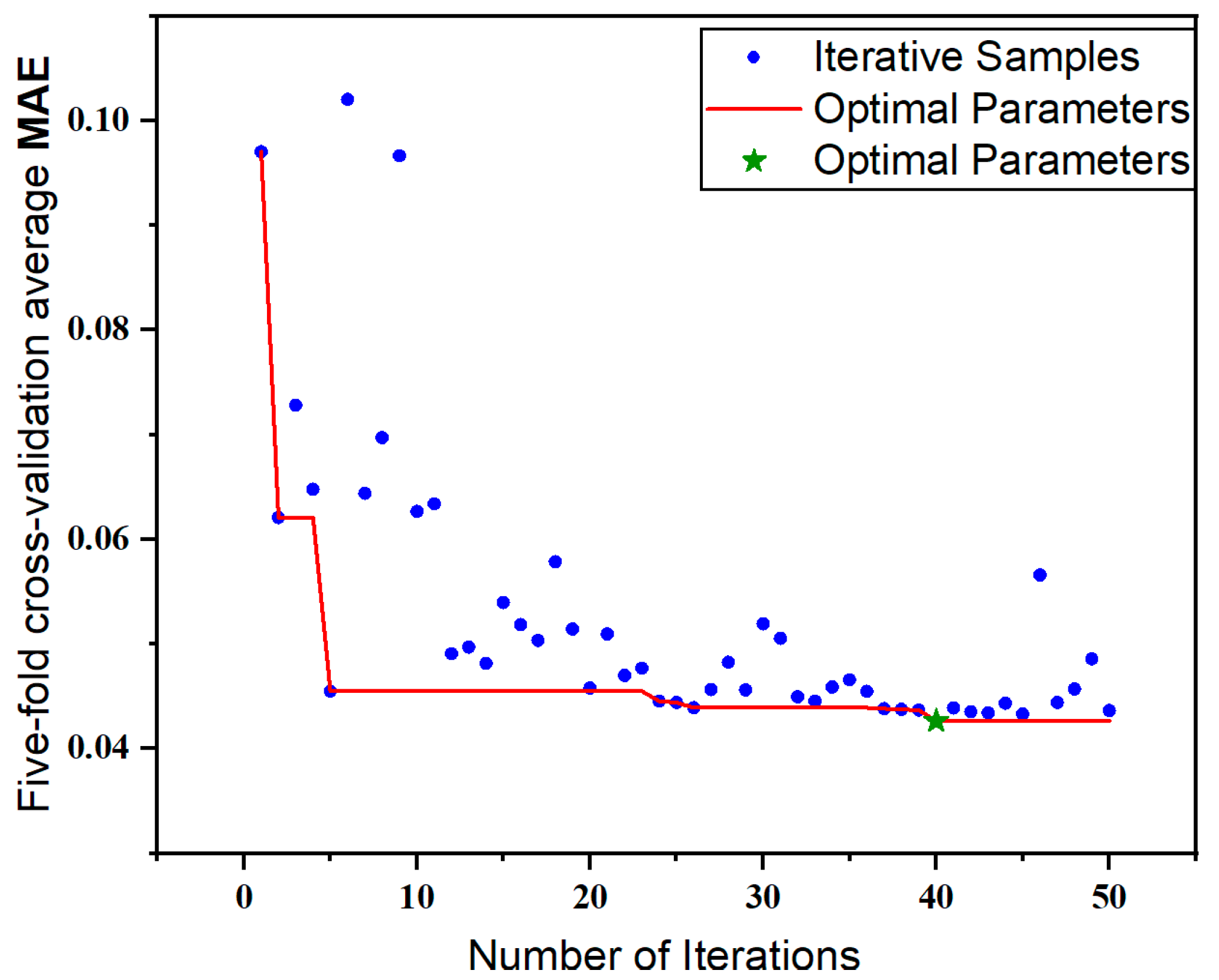
As shown in
Figure 6, BO-LightGBM identified the optimal hyperparameters during its 50th iteration:learning_rate = 0.051, num_leaves = 254, max_depth = 15, min_data_in_leaf = 45, feature_fraction = 0.978, bagging_fraction = 0.699, bagging_freq = 7, lambda_L1 = 9.289, lambda_L2 = 3.664, with the optimal loss function value of 0.0426.
3.4. Result Analysis
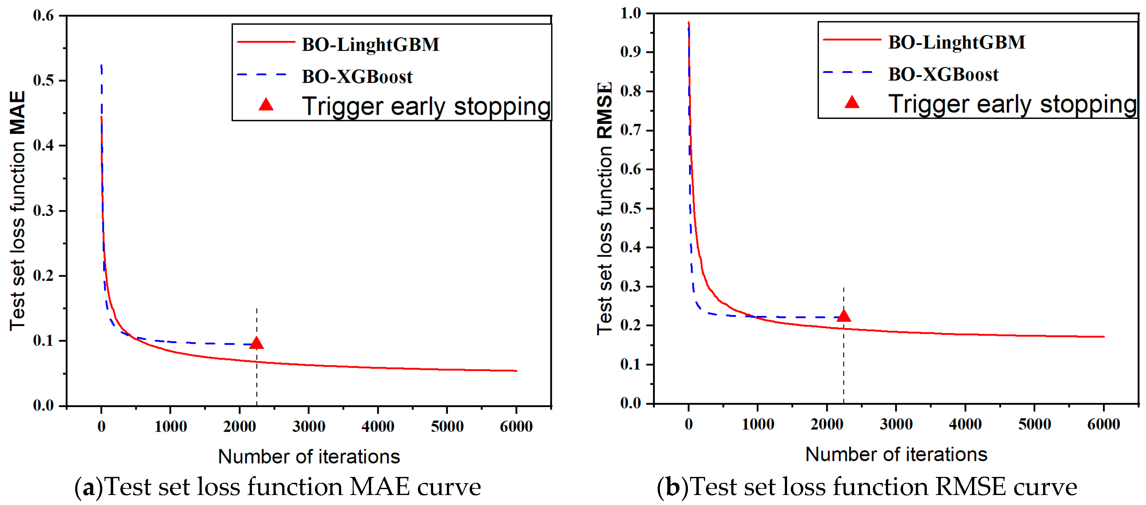
To evaluate the performance of the BO-LightGBM surrogate model, this study used the BO-XGBoost model as a comparative benchmark, trained under the same conditions. During the training process, as shown by the black dotted line in
Figure 7, the BO-XGBoost model triggered an early termination mechanism after 100 consecutive rounds with no improvement in the validation set MAE, ultimately achieving an MAE value of 0.095 on the test set. In contrast, the BO-LightGBM model demonstrated superior computational performance, with a test set MAE of only 0.0543. After normalization, the average computational error for BO-XGBoost was 1.4565 MPa, while for BO-LightGBM, it was reduced to 0.8325 MPa. These results indicate that BO-LightGBM significantly reduced the computational error by 42.84% compared to BO-XGBoost, demonstrating a clear accuracy advantage. Additionally, in terms of error distribution, the RMSE for BO-LightGBM (0.1718) outperformed that of BO-XGBoost (0.2214), further confirming its superior performance.
A comparison of the time efficiency between the two surrogate models and the traditional finite element simulation model is shown in
Table 6. The finite element simulation model requires 2580 s for simulation and cannot be directly used for rapid computation, as it is limited to a single predefined operating condition. In contrast, BO-XGBoost has a training time of 1104 s and a computation time of 0.92 s; BO-LightGBM required 559 s for training and 0.55 s for real-time computation. BO-LightGBM reduced training time by approximately 49.37% compared to BO-XGBoost and improved real-time performance by 40.22%. Consequently, BO-LightGBM was selected as the final stress calculation surrogate model.
3.5. Establishment of Displacement Surrogate Model
In this study, both the displacement surrogate model and the stress surrogate model adopt the same BO-LightGBM architecture. The operational condition samples were generated using the previously described Latin hypercube sampling method. While the two models share identical sampling schemes, their target data differ: the stress surrogate model employs equivalent stress obtained from finite element simulations, whereas the displacement surrogate model uses total displacement as its target variable. All sample data were derived exclusively from finite element simulations to ensure reliability.
The training process of the displacement surrogate model involved data preprocessing, feature selection, and model training, with performance optimized through cross-validation, consistent with the procedure used for the stress surrogate model. To evaluate predictive accuracy, the model outputs were compared against finite element simulation results. The results demonstrate that the displacement surrogate model effectively predicts maximum real-time displacement, achieving accuracy closely aligned with finite element outcomes. Although minor deviations are observed under certain complex operating conditions, the displacement surrogate model overall exhibits high predictive accuracy and stability while substantially enhancing computational efficiency, thereby confirming its suitability for engineering applications.
4. Structural Performance Assessment of the Digital Twin System Development
4.1. Digital Twin System Framework and Composition
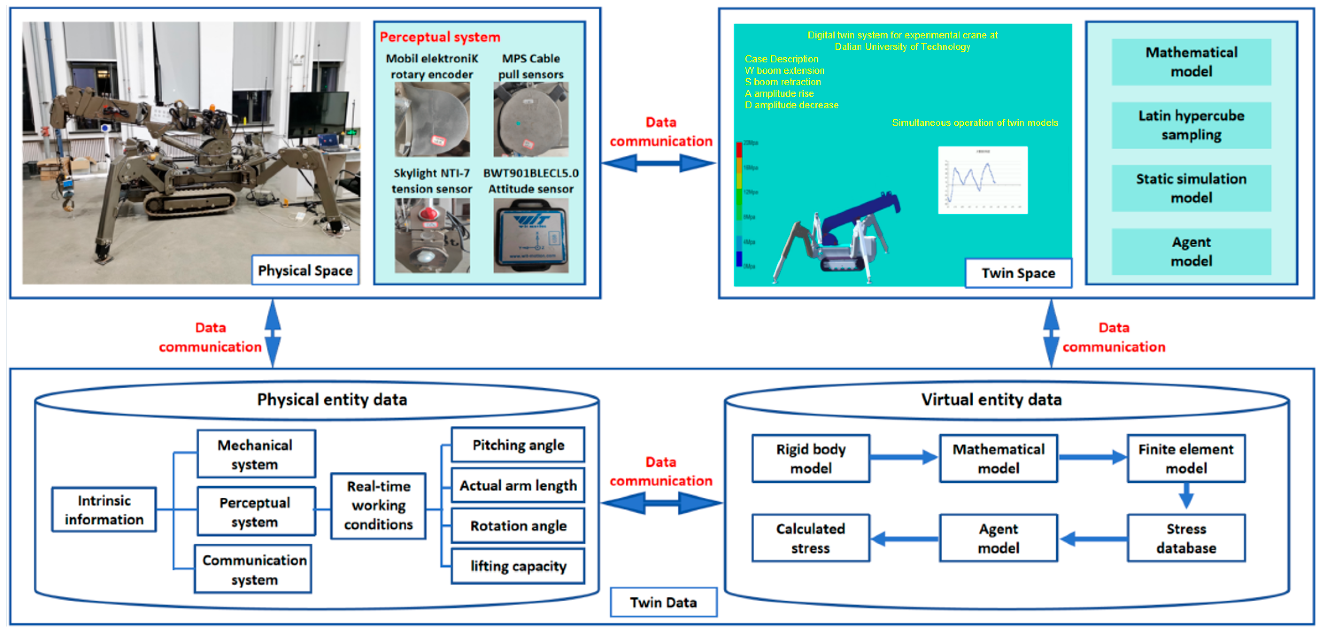
The digital twin system of a telescopic crane enables dynamic assessment and safety monitoring of structural performance through closed-loop interaction between the physical and twin spaces. The digital twin framework is illustrated in
Figure 8. The physical space comprises the crane entity, a multi-source sensor network (including pull-wire sensors, rotary encoders, attitude sensors, etc.), and an electro-hydraulic control system, which collect key operating condition data such as boom length, rotation angle, boom angle, and load weight in real time. The twin space integrates multi-dimensional digital models, including physical models, surrogate models, and finite element analysis models, and relies on the Unity 3D engine to achieve high-fidelity visualization of stress cloud maps, deformation analysis, and point cloud models. The system adopts a layered data interaction architecture, integrates multi-protocol sensor data through the data acquisition layer, and achieves efficient data synchronization between the industrial control computer, visualization platform, and stress calculation module based on a TCP dual-connection mechanism. Additionally, it utilizes a MySQL database for intelligent storage and management of operating condition data.
4.2. Unidirectional Performance Evaluation
4.2.1. Applied Load Assessment
Load assessment accurately determines the operational cycle of a telescopic crane by monitoring its real-time load status and identifying potential overload risks in a timely manner. The real-time load mass is detected by a Tian Guang NTIL tension sensor, with a permissible error of , which is used for online determination of the operational cycle. The specific rules are as follows:
- (1)
If , mark “operational cycle start”, indicating that the crane has entered the current operational cycle and has begun the load operation;
- (2)
If , mark “work cycle end”, indicating that the crane is in an unloaded state.
The real-time working radius
is a key parameter for load assessment and directly affects the determination of the rated load. The system uses sensors to monitor the real-time boom length
L and boom angle θ of the telescopic boom in real time, and calculates
using the following geometric formula:
The relationship between the real-time working radius
and the current rated load
can be found in the telescopic crane performance parameter table, which is then used to assess whether the current load status is safe. To intuitively display the load assessment results, they are quantified on a percentage basis. The load assessment index
is
Considering the working characteristics of telescopic cranes and the need to adapt to different working conditions, telescopic cranes frequently adjust the boom angle and boom length. During an operational cycle, if the boom angle increases or the boom length decreases, the real-time working radius decreases, the rated load increases, and the real-time load mass remains unchanged. In this case, no overload update will be triggered, and the original load assessment index will be maintained. However, if the boom is lowered or extended, the real-time working radius increases, the rated load decreases, and the real-time hoisting mass remains unchanged, may occur, causing an overload, and the load assessment index needs to be updated.
4.2.2. Material Strength Assessment
The calculated stress
at node
i is obtained through the BO-LightGBM stress surrogate model. According to the structural material parameter database, the allowable stress
of this node is known. As long as
is satisfied, the material strength of this node meets the requirements. The overall material strength of the telescopic crane is assessed using the material strength assessment index
S, which is calculated using the following formula:
4.2.3. Structural Stiffness Assessment
Structural stiffness assessment ensures that the telescopic boom can maintain sufficient deformation resistance after being subjected to specified loads and constraints. Structural stiffness reflects the ability of a structure to resist deformation caused by external forces. It is quantified by calculating the ratio of real-time displacement to allowable static displacement. As shown in Equation (7), the allowable displacement varies with the real-time boom length
L. The real-time allowable static displacement
is calculated based on the real-time boom length
L detected by the Milan MPS cable sensor. The displacement surrogate model is trained using the −Y direction displacement data of the finite element model established by extracting operating condition samples in
Section 2. If the maximum real-time displacement calculated by the surrogate model,
, is less than
, the structural stiffness meets the requirements. Therefore, the structural stiffness evaluation index
K is quantified by the following formula:
4.2.4. Fatigue Life Assessment
Using the BO-LightGBM surrogate model, the stress time series
of all nodes in an operational cycle is calculated based on the operating conditions of the telescopic crane within an operational cycle (real-time boom length
L, boom angle θ, and load mass mp). The rainflow counting method is applied to the stress time series
of node
j to break down the complex stress history into a series of independent cyclic loads, extracting the amplitude
and cycle number
of
k complete stress cycles. Based on Miner’s linear damage theory, the maximum cycle number
of the stress amplitude
is obtained through the Goodman straight line model-corrected material S-N curve. Before this operational cycle, the cumulative fatigue damage of this node is
. During this operational cycle, the fatigue damage
of node
j is
The fatigue life
F of node
j is
Then, the formula for quantifying the fatigue life assessment index
F of the target telescopic crane as a percentage is
4.2.5. Structural Assessment Visualization Interface
The structural assessment visualization interface is shown in
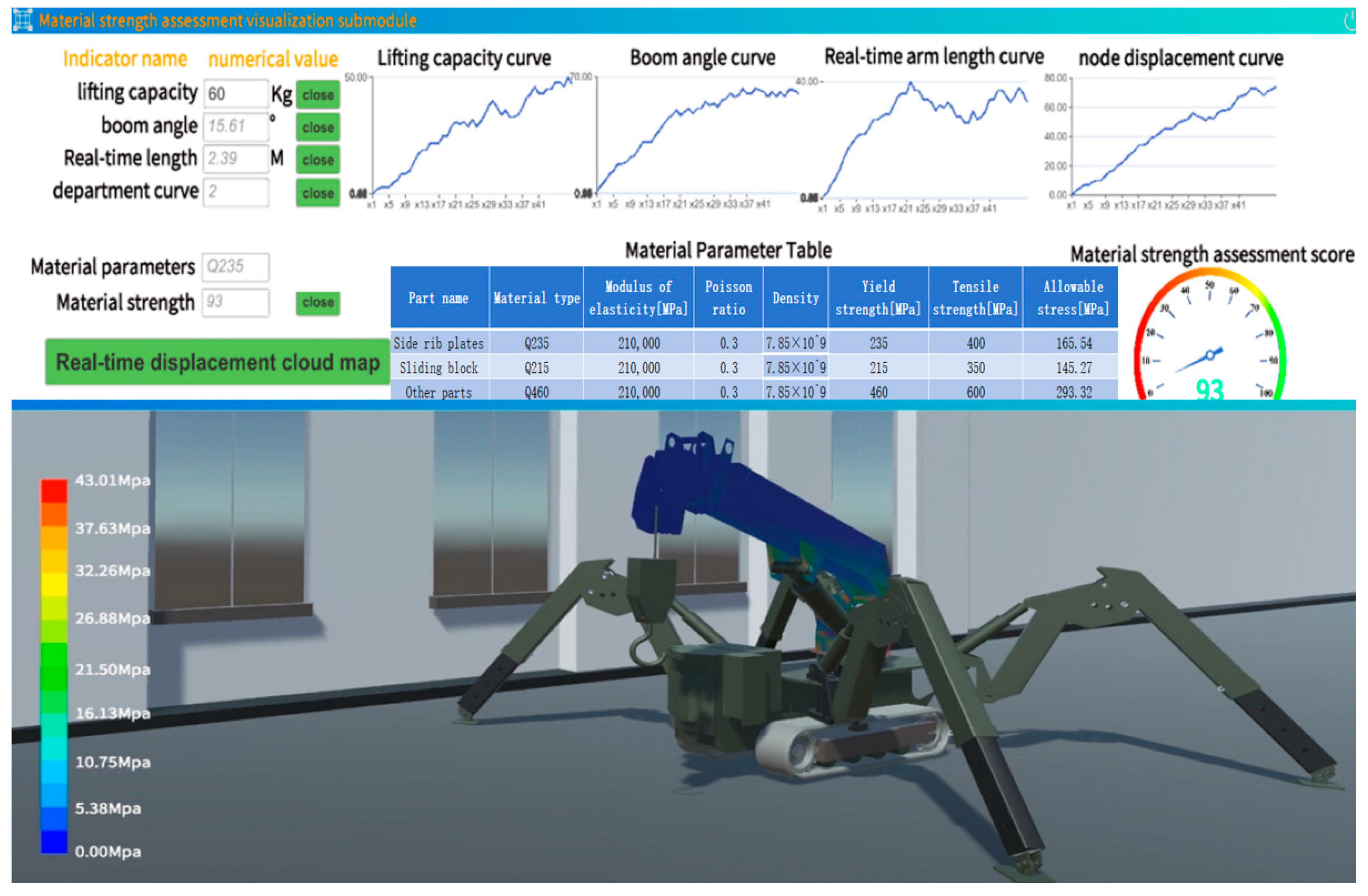
Figure 9. Real-time operating condition curves are generated based on the real-time operating condition parameters monitored by the sensors. By clicking the real-time stress cloud map button, the real-time operating condition information is sent to the Python (version 3.11.5)-side BO-LightGBM stress surrogate model via TCP communication. The surrogate model then transmits the stress data of all nodes to Unity 3D, updating the stress cloud map in the twin cloud map model. Based on the stress data from all current nodes, the stress cloud map legend is updated, a real-time assessment score is generated, and the structural assessment dashboard is refreshed.
Figure 9 also shows the material strength assessment interface.
4.3. Comprehensive Structural Performance Assessment
To conduct a long-term assessment of the structural performance of telescopic cranes throughout their full service life cycle, this research proposes a comprehensive assessment method based on the operational cycle. The core of the method involves extracting the most critical values of the four key performance indicators () during each operational cycle to form a performance indicator matrix. The assessment employs a comprehensive weighting strategy that combines the analytic hierarchy process (AHP) and the entropy weight method, taking into account both expert knowledge and the dynamic characteristics of objective data.
First, the weights of each indicator were calculated using the AHP method (
). Five experts from the field of mechanical engineering, representing both academia and industry, were invited to score the importance of the four evaluation criteria using a 1–9 scale, as shown in
Table 7. Based on the expert ratings, a judgment matrix A was constructed. The maximum eigenvalue of the judgment matrix A (
) and its corresponding eigenvector were calculated. After normalization, the initial weights (
) were obtained.
Subsequently, a consistency test is conducted to calculate the consistency ratio:
where
where
CI is the consistency index, n is the number of single indicators, RI is the average random consistency index. Since the judgment matrix is of the 4th order, refer to the table to determine that
is 1.12 [
29].
CR is the consistency ratio. If
, the matrix consistency is considered acceptable; otherwise, the judgment matrix is discarded. Finally, take the average of the judgment matrix A that passes the consistency check to obtain the final
.
Calculate the entropy weight method weights using the entropy weight method. First, extract the scores of each evaluation indicator for the last 100 operational cycles based on the operational cycle table to obtain the data matrix X, and then normalize the data matrix X.
Calculate the entropy value of the jth indicator . The entropy value reflects the degree of dispersion of the indicator data in different operational cycles: the smaller the , the greater the fluctuation of the indicator data (i.e., the higher the degree of differentiation), and the higher the weight that should be assigned.
Calculate the entropy weight method weight of each indicator based on the entropy value
:
Therefore, the entropy weight method weight matrix
is
Combining the two weight calculation methods, the comprehensive weight
is
Using the single performance indicator matrix and comprehensive weight of the current operational cycle, the final evaluation score is calculated as follows:
This score, , intuitively reflects the comprehensive status of structural performance under the current operational cycle and is displayed in real time on the main human–machine interaction interface.
5. Experimental Design
5.1. Experimental Platform Setup
The experimental platform in this research is based on the physical entity of the target telescopic crane. Through the supporting sensor system, key operating parameters such as boom length, load weight, boom angle, and swing angle are accurately detected in real time. Therefore, a three-axis strain gauge is additionally used to measure stress, thereby verifying the accuracy of the digital twin structural performance assessment.
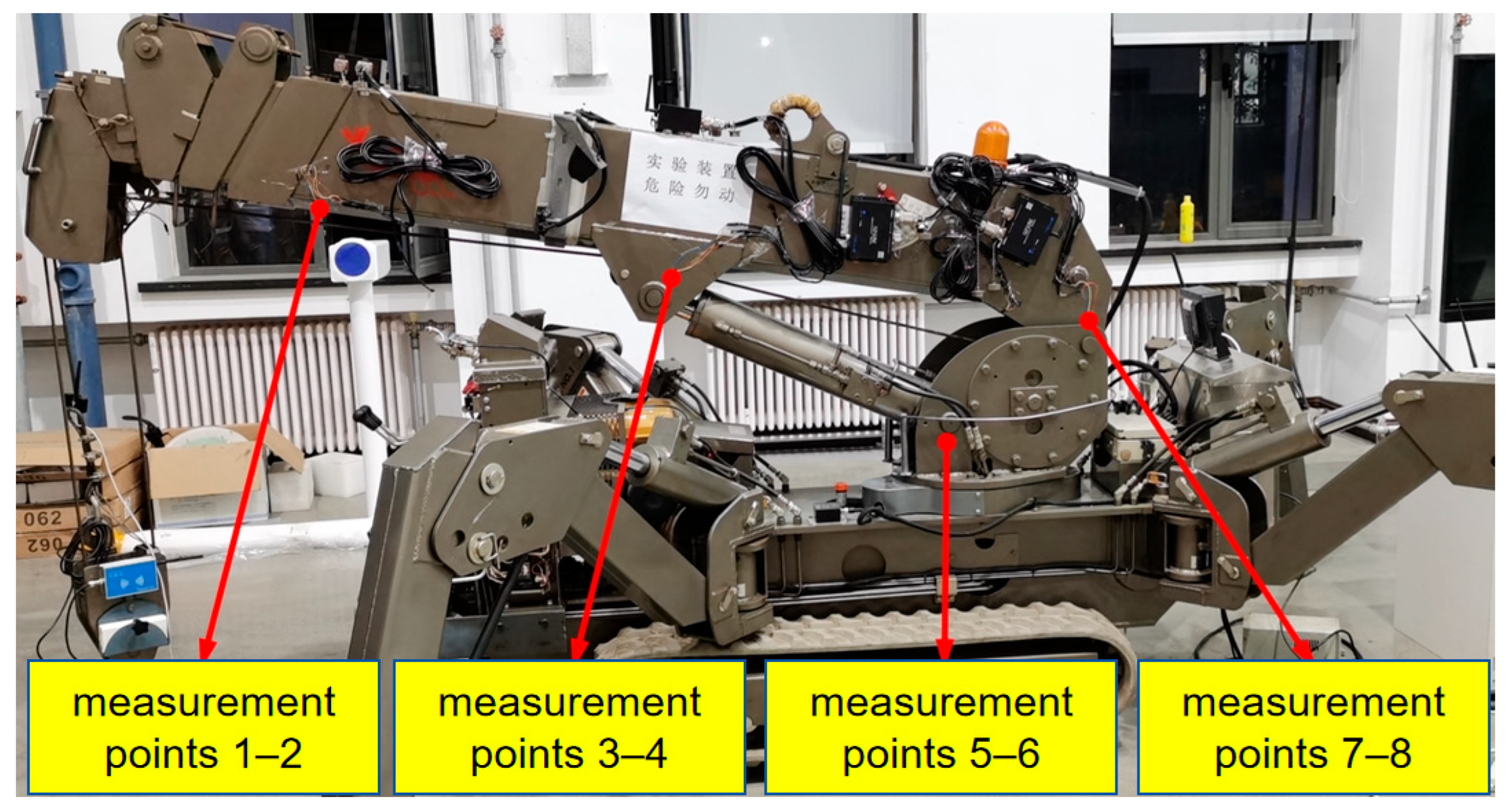
Due to the structural characteristics of telescopic arms, the second to fifth sections of the arm are coated with lubricating oil for telescoping purposes, making it impossible to attach three-axis strain gauges. Furthermore, the first section and the turntable are the parts of the telescopic arm that bear the heaviest loads. Therefore, a total of eight stress measurement points were selected on the first section and the turntable. The selected test points are all located at key structural parts that require close monitoring of stress changes. The belly plate of the telescopic arm is prone to large uniform stresses, while the hinge area is a thin-walled component with an open structure that is prone to stress concentration and material strength failure, making it an area that requires close verification. The locations of the eight stress measurement points are shown in
Figure 10.
In this study, all sensors underwent rigorous calibration prior to experimentation. Each measurement channel of the triaxial strain gauges was connected to the DH5908L dynamic stress meter. After the system warmed up and stabilized, the bridge parameters were configured using the accompanying software. During calibration, high-precision calibration resistors were connected to apply known standard electrical signals. This established an accurate conversion relationship between the data acquisition instrument’s output voltage and the strain value. Channel balance calibration was also completed to ensure consistent response across all channels, providing a reliable foundation for precise data acquisition in subsequent steps.
During data acquisition, the DH5908L wireless dynamic stress meter and the software-created test project established a Wi-Fi connection with the instrument. Parameters for each measurement channel were configured: selecting the 1/4-bridge configuration, setting the strain gauge resistance to 120Ω, setting the sensitivity coefficient K = 2.20, and calibrating the strain gauge array orientation (0°/45°/90°). The sampling frequency was set to 200 Hz with continuous sampling mode enabled. After parameter configuration, a hardware zeroing operation was performed to eliminate systematic errors. Subsequently, the data acquisition task was initiated for real-time monitoring of triaxial strain waveforms in the time domain, and data was saved in binary format to support subsequent stress analysis.
To ensure high precision and stability in data acquisition, this study implemented noise suppression measures at both the physical and software levels during measurement. Physically, all strain gauge leads were securely fastened to the telescopic arm to prevent cable sway during vibration, thereby avoiding induced electromotive force in the magnetic field and reducing noise interference. On the software side, the system employed anti-aliasing filters and low-pass filters to suppress high-frequency noise. Anti-aliasing filters restricted the introduction of high-frequency signals, preventing their aliasing into the effective bandwidth and thus avoiding signal distortion. Low-pass filters filtered out high-frequency noise exceeding the effective bandwidth, ensuring data accuracy and clear signal acquisition.
5.2. Material Strength Evaluation Experiment
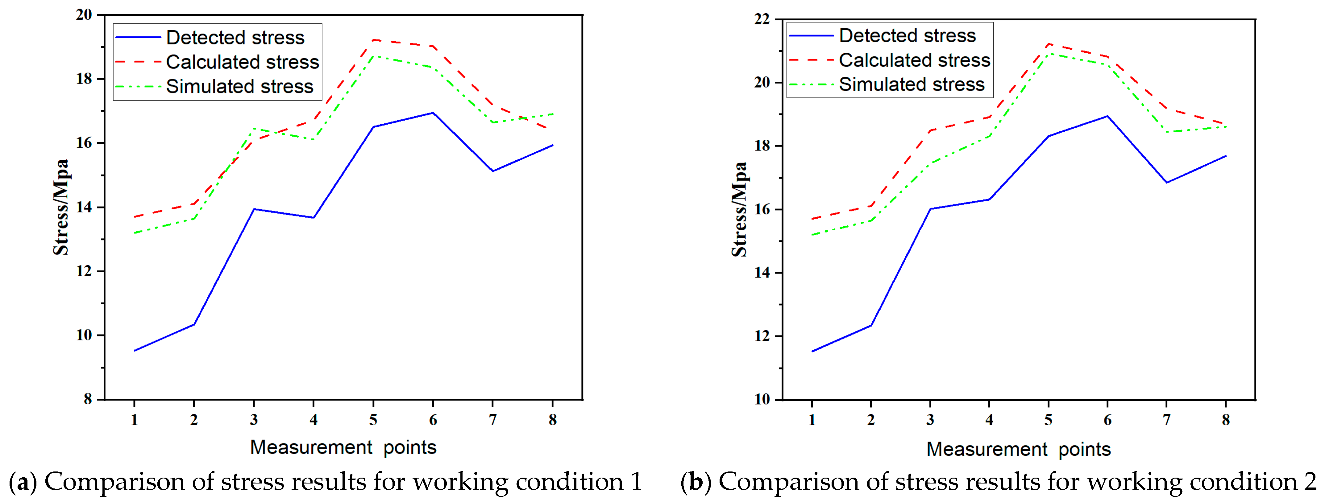
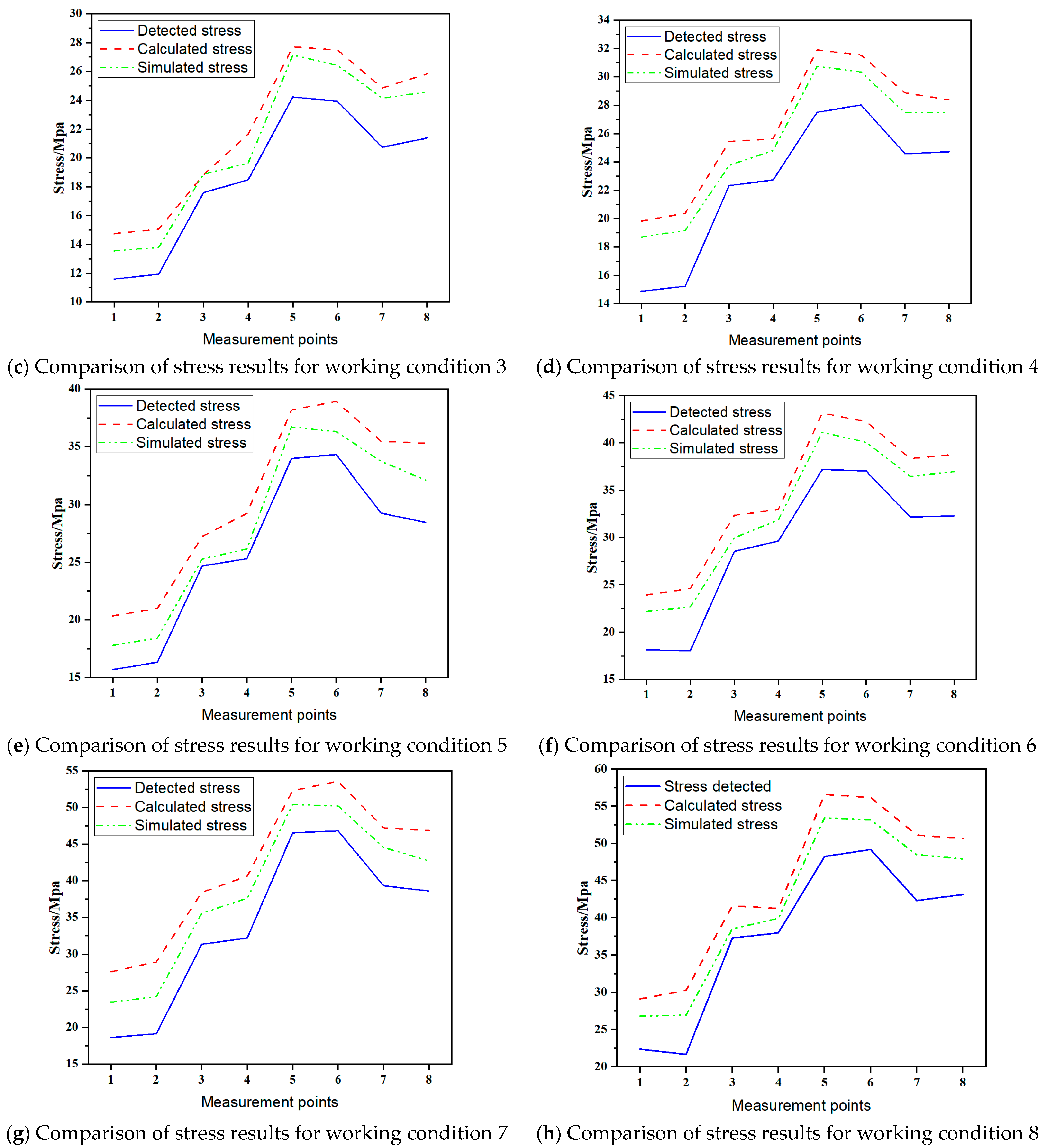
Four working conditions were selected for the target telescopic crane, and the stress detected at the eight measurement points shown in
Figure 10 was compared with the stress simulated by the finite element model and the stress calculated by the BO-LightGBM surrogate model. To prevent data leakage in the surrogate model, all comparison working conditions strictly avoided the use of Latin hypercube sampling points. Therefore, in order to obtain the finite element simulation stress under these working conditions, it was necessary to ensure that all other settings were consistent with the finite element model established in
Section 1, and only the working condition parameters were adjusted to compute the finite element simulation stress at the corresponding points under these conditions. The eight selected working conditions were as follows:
Working condition 1: the lifting device system is unloaded, the boom angle is 60°, and the boom length is 4.5 m.
Working condition 2: the lifting device system is unloaded, the boom angle is 30°, and the boom length is 7 m.
Working condition 3: the lifting device system is loaded with a 30 kg weight, the boom angle is 60°, and the boom length is 4.5 m.
Working condition 4: the lifting device system is loaded with a 30 kg weight, the boom angle is 30°, and the boom length is 7 m.
Working condition 5: the lifting device system is loaded with a 60 kg weight, the boom angle is 60°, and the boom length is 4.5 m.
Working condition 6: the lifting device system is loaded with a 60 kg weight, the boom angle is 30°, and the boom length is 7 m.
Working condition 7: the lifting device system is loaded with a 100 kg weight, the boom angle is 60°, and the boom length is 4.5 m.
Working condition 8: the lifting device system is loaded with a 100 kg weight, the boom angle is 30°, and the boom length is 7 m.
The test results indicate that, as shown in
Figure 11, the trends in the measured stress, simulated stress, and calculated stress at each test point under different working conditions are consistent. Specifically, under no-load conditions (working conditions 1 and 2),
Figure 11a,b demonstrate that the simulated and calculated stress curves are nearly identical. As the load mass increases, the discrepancy between the two also grows. Under the 100 kg load condition (operating conditions 7 and 8),
Figure 11g,h reveal the maximum deviation between the two, indicating that the surrogate model exhibits superior computational accuracy under no-load conditions compared to loaded conditions.
Through statistical analysis of the stress data from eight operating conditions and eight measurement points (
Table 8), the following conclusions were drawn:
The maximum detection error (the maximum error in the stress detected at symmetrical measurement points) is 1.09 MPa, proving that the detection data accurately reflects the actual stress distribution of the target telescopic arm.
The maximum simulation error (the maximum error between the finite element simulation and the detected stress) is 6.18 MPa. Considering model simplifications and experimental environment interference, this error is within an acceptable range, validating the reliability of the finite element model.
The maximum calculation error under no-load conditions (the maximum error between the surrogate model and the finite element simulation) is 0.76 MPa, confirming the accuracy of the stress surrogate model.
Under the 100 kg weight applied load condition, the maximum calculated error increased to 4.15 MPa due to the application of the stress load coefficient conversion method. However, reasonable accuracy was maintained, validating the effectiveness of the conversion method.
The maximum practical error (maximum discrepancy between the surrogate model and measured stress) occurred under the 100 kg load condition, reaching 8.98 MPa. This error primarily stems from two factors: finite element modeling and theoretical assumptions. First, to enhance computational efficiency, the finite element model employed shell elements for discretization. These elements inherently impose geometric approximations, leading to a systematic overestimation of simulated stresses. Consequently, the surrogate model, constructed based on this simulation data, exhibits an overestimation bias. Second, although a linear relationship between load mass and stress is expected under linear elasticity and small deformation assumptions, slight nonlinear structural responses may occur under high-load conditions. Combined with the idealization introduced by stress conversion factors, this further contributes to computational deviations.
Despite these errors, the digital twin system developed in this study accurately reflects the structural stress distribution under low-load conditions. Under high-load conditions, while the error increases, it remains within the system’s acceptable range and exhibits a conservative bias: when the surrogate model’s output reaches the stress warning threshold, the actual structural stress is typically lower than this value, ensuring that the assessment results possess a certain safety margin. From the perspective of the core function of digital twins, the primary objective is to accurately reproduce the overall morphology and trend of structural stress distribution. The results from the eight load cases presented in
Figure 11 consistently demonstrate that the surrogate model exhibits good rationality in predicting stress distribution characteristics, thereby validating the effectiveness and reliability of this material strength assessment module in engineering applications.
5.3. Fatigue Life Simulation Experiment Verification
Since the fatigue life of telescopic cranes is difficult to measure directly through experiments, this study employs numerical simulation methods for verification. Without considering the existing damage to the structure, the results of the nCode finite element simulation were compared with the fatigue life calculation results from the digital twin system’s assessment submodule. The calculation principles of the two methods are consistent, with the main difference being the stress input source: the digital twin system uses the BO-LightGBM surrogate model to calculate stress, while the nCode simulation is based on a multi-time-step finite element model. The focus of the experimental verification was to determine whether the fatigue life assessment submodule could accurately calculate the fatigue damage accumulation from the stress data output by the BO-LightGBM surrogate model, using the integrated rainflow counting method and the S-N curve algorithm modified by the Goodman linear model. The experimental data (
Table 9) show that the error in the fatigue life calculation results obtained by the two methods is only 2.86%, indicating high calculation accuracy. Given that the BO-LightGBM surrogate model has been proven to fit the finite element calculation results well, this experiment further validates that the developed fatigue life assessment algorithm can replicate the assessment process of the nCode software with high accuracy, demonstrating that the system can achieve long-term and reliable fatigue life monitoring and assessment based on real-time operational cycle data.
6. Conclusions
This research proposes a method for the structural performance assessment of a telescopic crane throughout its entire service life cycle based on digital twins. By integrating finite element simulation and the Bayesian optimization LightGBM surrogate model (BO-LightGBM), the method enables comprehensive assessment of structural strength, structural stiffness, and fatigue life. The experimental results show that, in terms of calculation accuracy, compared with the benchmark BO-XGBoost model, the BO-LightGBM surrogate model reduces the mean absolute error (MAE) by 42.84% and improves the root mean square error (RMSE) by 22.4%. In multi-condition stress prediction, the maximum calculation error of the model under no-load conditions was 0.76 MPa (relative error: 1.5%), verifying the accuracy of the stress prediction model. Under a 100 kg load condition, after applying the dynamic conversion method of the stress load coefficient, the maximum calculation error was 4.15 MPa (relative error: 8.3%), confirming the effectiveness of the dynamic conversion method. System-level verification showed that the reference error between the finite element simulation results and the actual measured stress was 6.18 MPa, validating the reliability of the basic finite element model. The maximum deviation between the surrogate model’s predicted stress and the actual measured stress was 8.98 MPa, indicating that the material strength assessment module of the digital twin system can effectively calculate the structural stress distribution. In terms of fatigue life assessment, the deviation between the results of this method and the results calculated by nCode (version 2022 R2) software was only 2.86%, demonstrating high calculation accuracy. This method upgrades traditional offline single-index analysis to an online comprehensive assessment covering multiple indices such as material strength, structural stiffness, and fatigue life. It also establishes a three-level mapping architecture of “physical entity-simulation model-surrogate model,” significantly improving assessment efficiency while ensuring calculation accuracy, thus providing more scientific and reliable technical support for the structural safety monitoring of construction machinery.
The linear stress–load coefficient conversion method employed in this study is based on the assumption that, within the applied load range not exceeding the yield material strength, the relationship between applied load and stress generally conforms to the linear elasticity hypothesis and the small deformation hypothesis. Within this load range, the increase in load mass should exhibit a linear relationship with the stress variation at finite element nodes. This linear relationship performs well under low applied loads. However, under high applied load conditions, the structural response may exhibit slight nonlinear behavior. Combined with the idealization introduced by the stress conversion coefficient, this can lead to minor computational deviations. Although this study employs a simplified linear model for calculations, the limitations of this assumption may impact model accuracy under extreme operating conditions. Future research may consider incorporating more complex nonlinear models or expanding the applied load range through Latin hypercube sampling to enhance the representativeness of sample data, thereby improving the model’s predictive accuracy under complex applied load conditions.
The stress calculation surrogate model proposed in this study was trained on a specific type of telescopic crane. When transferring this model to other crane types in practical applications, recalibration may be necessary. Significant differences in structural design and applied load distribution may exist across crane types. Therefore, model validation and retraining are recommended for new crane variants. This process can be achieved by adjusting existing training data or generating new datasets through finite element simulations of novel cranes to retrain the model, ensuring its applicability and accuracy.
Future research should focus on real-time deployment and large-scale monitoring. With the continuous advancement of IoT technology and digital twin systems, real-time monitoring systems can provide instant feedback to ensure crane safety during operations and enable timely early warnings and responses to potential failures. To achieve efficient management of large-scale equipment, future research must prioritize addressing technical bottlenecks such as data processing, storage, and computational efficiency, ensuring the capability for parallel monitoring and comprehensive optimization of multiple devices. Simultaneously, as data acquisition technologies advance, integrating data fusion with artificial intelligence will become pivotal for enhancing evaluation precision and intelligence. By merging data from diverse sensors (e.g., vibration, temperature, displacement) and applying AI techniques like deep learning and machine learning, the automation level and predictive accuracy of structural health assessment can be significantly improved. This will provide more advanced and efficient technical support for the long-term monitoring and intelligent maintenance of construction machinery.
Author Contributions
Conceptualization, X.C. and S.C.; methodology, X.C. and S.C.; software, K.L.; validation, Q.M., S.C. and K.L.; formal analysis, K.L.; investigation, Q.M.; resources, X.C. and Q.M.; data curation, S.C. and Q.M.; writing—original draft preparation, S.C.; writing—review and editing, S.C.; visualization, K.L.; supervision, X.C.; project administration, X.C.; funding acquisition, X.C. All authors have read and agreed to the published version of the manuscript.
Funding
This research was funded by the National Key R&D Program of China (Grant No. 2024YFD2400200) and the National Natural Science Foundation of China (Grant No. 52275088).
Institutional Review Board Statement
Not applicable.
Informed Consent Statement
Not applicable.
Data Availability Statement
The data presented in this study are available on request from the corresponding author due to the proprietary nature of the crane model parameters and simulation configurations.
Conflicts of Interest
The authors declare no conflicts of interest.
References
- Sanaz, S.; Soltanmohammadlou, N.; Rahnamayiezekavat, P. A systematic review of scholarly works addressing crane safety requirements. Saf. Sci. 2021, 133, 105002. [Google Scholar] [CrossRef]
- Zhang, X.; Zhang, W.; Jiang, L.; Zhao, T. Identification of critical causes of tower-crane accidents through system thinking and case analysis. J. Constr. Eng. Manag. 2020, 146, 04020071. [Google Scholar] [CrossRef]
- Rølvåg, T.; Stranden, Ø. Digital Twin Based Structural Health Monitoring of Offshore Crane. In Proceedings of the ASME 2022 41st International Conference on Ocean, Offshore and Arctic Engineering, American Society of Mechanical Engineers Digital Collection, Hamburg, Germany, 21–30 July 2021; pp. 136–145. [Google Scholar]
- Moi, T.; Cibicik, A.; Rølvåg, T. Digital twin based condition monitoring of a knuckle boom crane: An experimental study. Eng. Fail. Anal. 2020, 112, 104–123. [Google Scholar] [CrossRef]
- He, X.W.; Lai, X.N.; Yang, L.L.; Song, X.G. Mechanism and data-driven digital twin design of gantry crane. In Proceedings of the 17th China CAE Engineering Analysis Technology Conference, Deqing, China, 12 November 2021; pp. 21–28. (In Chinese). [Google Scholar]
- Fu, L.; She, L.; Yan, D.; Zhang, P.; Long, X. Fatigue damage prediction model for arm systems based on BiLSTM neural networks with embedded physics information and attention mechanism. J. Mech. Eng. 2024, 60, 205–215. (In Chinese) [Google Scholar]
- Wang, Q.; Yan, B.; Chen, Y.; Deng, M.; Cai, Y. Dynamic structural digital twin method based on order reduction model and data-driven approach. Appl. Math. Mech. 2023, 44, 757–768. (In Chinese) [Google Scholar]
- Lai, X.; Wang, S.; Guo, Z.; Zhang, C.; Sun, W.; Song, X. Designing a shape–performance integrated digital twin based on multiple models and dynamic data: A boom crane example. J. Mech. Des. 2021, 143, 71–89. [Google Scholar] [CrossRef]
- Hussain, M.; Ye, Z.; Chi, H.; Hsu, S. Predicting degraded lifting capacity of aging tower cranes: A digital twin-driven approach. Adv. Eng. Inform. 2024, 59, 102310. [Google Scholar] [CrossRef]
- Liu, P.; Xing, L.; Liu, Y.; Zheng, J.Y. Strength Analysis and Optimal Design for Main Girder of Double-Trolley Overhead Traveling Crane Using Finite Element Method. J. Fail. Anal. Prev. 2014, 14, 76–86. [Google Scholar] [CrossRef]
- Tkachev, A.; Tkachev, A.; Predrag, D.; Prokopovych, I.; Kostina, M. Static Stiffness of the Crane Bridges Under Moving Load Distribution. In Proceedings of the 3rd Grabchenko’s International Conference on Advanced Manufacturing Processes, Dessa, Ukrain, 7–10 September 2021; pp. 43–52. [Google Scholar]
- Chen, L.; Liu, G.; Ding, K. Development and engineering application of fatigue life prediction software for lifting machinery. China Saf. Sci. Technol. 2016, 12, 138–145. (In Chinese) [Google Scholar]
- Li, Y. Fatigue life analysis of bridge crane main beam welds based on hot stress method. Comput.-Aided Eng. 2014, 23, 44–49. (In Chinese) [Google Scholar]
- Yan, B.; Ma, P.; Huang, Z.; He, C. Research on a safety evaluation system for lifting machinery based on fuzzy analytic hierarchy process. Autom. Instrum. 2024, 8, 155–158. (In Chinese) [Google Scholar]
- Zheng, Y.; Zhao, F.; Wang, Z. Fault diagnosis system of bridge crane equipment based on fault tree and Bayesian network. Int. J. Adv. Manuf. Technol. 2019, 105, 3605–3618. [Google Scholar] [CrossRef]
- Chen, D.; Li, Y.; Liu, K.; Li, Y. A physics-informed neural network approach to fatigue life prediction using small quantity of samples. Int. J. Fatigue 2023, 166, 107–124. [Google Scholar] [CrossRef]
- Schmid, S.; Richstein, R.; Schröder, K. Integration of Fatigue Estimation into Experimentable Digital Twins for Structural Applications. In Proceedings of the European Workshop on Structural Health Monitoring (EWSHM 2022), Palermo, Italy, 4–7 July 2022; Springer: Cham, Switzerland, 2023; pp. 423–432. [Google Scholar]
- Feng, X.; Jiang, J.; Feng, Y. Reliability evaluation of gantry cranes based on fault tree analysis and Bayesian network. J. Intell. Fuzzy Syst. 2020, 38, 3129–3139. [Google Scholar] [CrossRef]
- GB/T 700-2006; Carbon Structural Steels. Standard Press of China: Beijing, China, 2006.
- GB/T 1591-2008; High Strength Low Alloy Structural Steels. Standard Press of China: Beijing, China, 2008.
- GB/T 3811-2008; Design Rules for Cranes. Standard Press of China: Beijing, China, 2008.
- Zhao, J.; Dong, Q.; Xu, G.; Li, H.; Lu, H. A fast prediction method of fatigue life for crane structure based on Stacking ensemble learning model. J. Eng. Appl. Sci. 2024, 71, 207–213. [Google Scholar] [CrossRef]
- Chen, Z.; Li, Z.; Huang, C.; Zhang, G.; Yu, H. Safety Assessment Method of Bridge Crane Based on Cluster Analysis and Neural Network. Procedia Comput. Sci. 2018, 131, 477–484. [Google Scholar] [CrossRef]
- Xu, X.; Liu, C.; Li, J.; Miao, Y. Trajectory clustering for SVR-based Time of Arrival estimation. Ocean. Eng. 2022, 259, 111–121. [Google Scholar] [CrossRef]
- Huang, Y.; Liu, Y.; Li, C.; Wang, C. GBRTVis: Online analysis of gradient boosting regression tree. J. Vis. 2019, 22, 125–140. [Google Scholar] [CrossRef]
- Ke, G.; Meng, Q.; Finley, T.; Wang, T.; Chen, W.; Ma, W.; Ye, Q.; Liu, T. LightGBM: A Highly Efficient Gradient Boosting Decision Tree. In Proceedings of the Neural Information Processing Systems, Long Beach, CA, USA, 10–16 December 2017; pp. 134–146. [Google Scholar]
- Jiang, G.; Wang, W. Error estimation based on variance analysis of k-fold cross-validation. Pattern Recognit. 2017, 69, 94–106. [Google Scholar] [CrossRef]
- Chen, T.; Guestrin, C. XGBoost: A Scalable Tree Boosting System. In Proceedings of the 22nd ACM SIGKDD International Conference on Knowledge Discovery and Data Mining, New York, NY, USA, 13–17 August 2016; pp. 785–794. [Google Scholar]
- Min, C.; Gang, C. Evaluation of Public Transportation Service Satisfaction in a Highland City Using the AHP-Multi-Level Fuzzy Comprehensive Evaluation Method. Inn. Mong. Highw. Transp. 2023, 5, 35–40. (In Chinese) [Google Scholar]
Figure 1.
Sampling distribution of telescopic crane working conditions.
Figure 1.
Sampling distribution of telescopic crane working conditions.
Figure 2.
Boundary condition setup.
Figure 2.
Boundary condition setup.
Figure 3.
nCode simulation life cloud diagram.
Figure 3.
nCode simulation life cloud diagram.
Figure 4.
LightGBM algorithm implementation flow.
Figure 4.
LightGBM algorithm implementation flow.
Figure 5.
BO-XGBoost hyperparameter optimization history.
Figure 5.
BO-XGBoost hyperparameter optimization history.
Figure 6.
BO-LightGBM hyperparameter optimization history.
Figure 6.
BO-LightGBM hyperparameter optimization history.
Figure 7.
Test set loss function curves.
Figure 7.
Test set loss function curves.
Figure 8.
Digital twin system framework diagram.
Figure 8.
Digital twin system framework diagram.
Figure 9.
Structural assessment visualization interface.
Figure 9.
Structural assessment visualization interface.
Figure 10.
Stress measurement points.
Figure 10.
Stress measurement points.
Figure 11.
Comparison of stress results under different working conditions.
Figure 11.
Comparison of stress results under different working conditions.
Table 1.
Calculation table for telescoping arm lengths.
Table 1.
Calculation table for telescoping arm lengths.
| | | | |
|---|
| | | | |
| | | | |
| | | | Fourth gear |
Table 2.
Target crane material parameters.
Table 2.
Target crane material parameters.
| Part Name | Material Type | Modulus of Elasticity [MPa] | Poisson Ratio | Density | Yield Strength [MPa] | Tensile Strength [MPa] |
|---|
| Side rib plates | Q235 | 210,000 | 0.3 | 7.85 × 10⁻⁹ | 235 | 400 |
| Sliding block | Q215 | 210,000 | 0.3 | 7.85 × 10⁻⁹ | 215 | 350 |
| Other parts | Q460 | 210,000 | 0.3 | 7.85 × 10⁻⁹ | 460 | 600 |
Table 3.
Z-direction displacement time steps of the boom cylinder piston.
Table 3.
Z-direction displacement time steps of the boom cylinder piston.
| Lifting and Swing Time Steps | Z-Direction Displacement
/[mm] | Maximum Boom Angle
Time Step | Z-Axis Displacement
/[mm] | Decreasing Amplitude Time Step | Z-Axis Displacement
/[mm] |
|---|
| 1 | 0 | 6 | 271.42 | 11 | 271.42 |
| 2 | 42.62 | 7 | 271.42 | 12 | 150.18 |
| 3 | 93.6 | 8 | 271.42 | 13 | 93.6 |
| 4 | 150.18 | 9 | 271.42 | 14 | 42.62 |
| 5 | 210.1 | 10 | 271.42 | 15 | 0 |
Table 4.
BO-XGBoost parameter tuning table.
Table 4.
BO-XGBoost parameter tuning table.
| Hyperparameters | Sampling Range | Sampling Method |
|---|
| learning_rate | | Logarithmic scale sampling |
| max_depth | | Uniform integer sampling |
| min_child_weight | | Uniform integer sampling |
| feature_fraction | | Uniform continuous sampling |
| bagging_fraction | | Uniform continuous sampling |
| lambda_L1 | | Uniform continuous sampling |
| lambda_L2 | | Uniform continuous sampling |
Table 5.
BO-LightGBM parameter tuning table.
Table 5.
BO-LightGBM parameter tuning table.
| Hyperparameters | Sampling Range | Sampling Method |
|---|
| learning_rate | | Logarithmic scale sampling |
| num_leaves | | Uniform integer sampling |
| max_depth | | Uniform integer sampling |
| min_data_in_leaf | | Uniform integer sampling |
| feature_fraction | | Uniform continuous sampling |
| bagging_fraction | | Uniform continuous sampling |
| bagging_freq | | Uniform integer sampling |
| lambda_L1 | | Uniform continuous sampling |
| lambda_L2 | | Uniform continuous sampling |
Table 6.
Comparison of training and computational time across different models.
Table 6.
Comparison of training and computational time across different models.
| Model | Simulation/Training Time/[s] | Real-Time Computation Time/[s] |
|---|
| Finite element simulation model | 2580 | \ |
| BO-XGBoost | 1104 | 0.92 |
| BO-LightGBM | 559 | 0.55 |
Table 7.
1–9 scale method.
Table 7.
1–9 scale method.
| Scale | |
|---|
| 1 | Indicator i and indicator j are equally important |
| 3 | Indicator i is slightly more important than indicator j |
| 5 | Indicator i is significantly more important than indicator j |
| 7 | Indicator i is strongly more important than indicator j |
| 9 | Indicator i is extremely important compared to indicator j |
| 2, 4, 6, 8 | Indicator i is of intermediate importance relative to indicator j |
Table 8.
Statistics of stress results under different working conditions.
Table 8.
Statistics of stress results under different working conditions.
| Name | Maximum Measurement Error
/[MPa] | Maximum Simulation Error
/[MPa] | Maximum Calculation Error
/[MPa] | Maximum Actual Error
/[MPa] |
|---|
| Condition 1 | 0.82 | 3.6 | 0.66 | 4.18 |
| Condition 2 | 0.64 | 3.1 | 0.76 | 3.74 |
| Condition 3 | 0.89 | 3.41 | 2.01 | 4.45 |
| Condition 4 | 0.52 | 3.93 | 1.67 | 5.14 |
| Condition 5 | 0.81 | 4.48 | 3.09 | 6.85 |
| Condition 6 | 1.09 | 4.66 | 2.38 | 6.62 |
| Condition 7 | 0.84 | 5.42 | 4.15 | 8.98 |
| Condition 8 | 0.95 | 6.18 | 3.33 | 8.81 |
Table 9.
Comparison of the results of the two fatigue life assessment methods.
Table 9.
Comparison of the results of the two fatigue life assessment methods.
| Evaluation Method | Fatigue Life | Service Life/[a] | Calculation Error/[%] |
|---|
| nCode finite element method | 4.078 × 10⁵ | 25.49 | 2.8 |
| Fatigue life assessment submodule | 3.962 × 10⁵ | 24.76 |
| Disclaimer/Publisher’s Note: The statements, opinions and data contained in all publications are solely those of the individual author(s) and contributor(s) and not of MDPI and/or the editor(s). MDPI and/or the editor(s) disclaim responsibility for any injury to people or property resulting from any ideas, methods, instructions or products referred to in the content. |
© 2025 by the authors. Licensee MDPI, Basel, Switzerland. This article is an open access article distributed under the terms and conditions of the Creative Commons Attribution (CC BY) license (https://creativecommons.org/licenses/by/4.0/).
