Abstract
Reliable LiDAR point clouds are essential for perception in robotics and autonomous driving. However, adverse weather conditions introduce substantial noise that significantly degrades perception performance. To tackle this challenge, we first introduce a novel, point-wise annotated dataset of over 800 scenes, created by collecting and comparing point clouds from real-world adverse and clear weather conditions. Building upon this comprehensive dataset, we propose the Spatial Context-Aware Point Cloud Encoder Network (SCOPE), a deep learning framework that identifies noise by effectively learning spatial relationships from sparse point clouds. SCOPE partitions the input into voxels and utilizes a Voxel Spatial Feature Extractor with contrastive learning to distinguish weather-induced noise from structural points. Experimental results validate SCOPE’s effectiveness, achieving high Intersection-over-Union (mIoU) scores in snow (88.66%), rain (92.33%), and fog (88.77%), with a mean mIoU of 89.92%. These consistent results across diverse scenarios confirm the robustness and practical effectiveness of our method in challenging environments.
1. Introduction
LiDAR sensors are fundamental components in autonomous driving systems, emitting laser pulses and capturing their reflections to produce high-resolution 3D point clouds for accurate environmental perception [1,2,3,4]. However, the LiDAR data available in most large-scale autonomous driving datasets tend to be artificially “clean” and lack the imperfections encountered in real-world scenarios [5,6,7]. Adverse weather conditions such as rain and snow can significantly degrade the quality of LiDAR sensor data. Atmospheric particles like raindrops, fog, and snowflakes cause scattering, refraction, and absorption of the laser beams, resulting in point loss and noise artifacts, leading to significant noise [8,9,10]. This information degradation poses a serious challenge for perception systems in autonomous robots and self-driving vehicles operating under adverse weather, leading to a notable drop in performance [11,12,13,14]. Driver fatality rates increase significantly during inclement weather, highlighting the critical need for robust perception data under such conditions.
To ensure the robustness of autonomous driving systems under various weather conditions, removing weather-induced noise points from point cloud data is a crucial task. Several point cloud denoising methods have been developed, which can be broadly categorized into statistical and deep learning-based approaches. Statistical methods typically filter noise by analyzing the distribution patterns of point clouds [15], while effective on smaller datasets, these methods often demand substantial computational resources when applied to large-scale point clouds [16]. In contrast, deep-learning-based methods leverage the feature-learning capabilities of neural networks to model noise patterns directly from the input data [5]. Existing deep learning approaches are further classified based on the input format into range-image-based and 3D-point-cloud-based methods. Range-image-based techniques project 3D point clouds onto 2D range images, which can introduce a loss of spatial information and degrade denoising performance, particularly in complex scenarios. On the other hand, 3D-point-cloud-based methods operate directly on raw point sets, better preserving spatial structures and geometric information, leading to more effective denoising [17]. Despite their promising results, deep learning methods often suffer from limited interpretability, posing challenges for understanding and improving their behavior. Moreover, addressing the challenge of mitigating noise induced by adverse weather conditions is non-trivial due to the inherent characteristics of LiDAR sensors, the sparsity of the point cloud data, occlusions introduced by the noise, and the heterogeneous density of the noise itself.
In addition, LiDAR perception under adverse weather conditions presents a unique challenge compared to general segmentation tasks, as it is difficult to obtain labeled data for noise. Unlike objects such as cars or pedestrians, noise points do not exhibit consistent shapes and can distort or occlude the structure of real objects, making point-wise labeling challenging. To address this, synthetic data generation and noise augmentation models have been proposed; however, such data still fail to accurately represent real-world scenarios, while some studies have provided point-level adverse weather datasets, they remain insufficient for extreme cases, such as heavy fog, which significantly affect real-world driving conditions.
To address the challenge of point cloud corruption under adverse weather conditions, we propose SCOPE (Spatial Context-Aware Point Cloud Encoder)—a denoising framework that leverages spatially encoded voxel representations to effectively capture geometric relationships among points. Our approach partitions the input point cloud into fixed-size voxels and extracts features based on the intra-voxel geometric structure by applying the Voxel Feature Extractor (VFE). A Spatial Attentive Pooling (SAP) module then utilizes the geometrical encoded features to train he context across the features of the neighboring K-points, enabling the network to learn discriminative representations through contrastive learning. This process significantly enhances the separation between noise and valid points. Furthermore, to validate our network on real world dataset, we introduce a noise point annotation strategy to construct a point-wise annotated dataset in adverse weather conditions. By comparing scenes captured under clean and adverse weather within the same sensor configuration and environment, we are able to accurately identify and label noise points. This natural data generation method provides realistic training and evaluation scenarios. Our experiments demonstrate that the proposed framework effectively filters noise and improves point cloud segmentation performance in challenging weather conditions. Our contributions are as follows:
- We introduce a network that effectively captures the spatial characteristics among points within a voxel. This allows us to discern geometric relationships between points even in sparse conditions. Additionally, by emphasizing the differences between clusters through contrastive learning, we facilitate effective segmentation learning.
- To facilitate the acquisition of point-wise annotated data under adverse weather conditions, we propose a noise point acquisition and labeling strategy. Leveraging this method, we collect point cloud scenes captured in real-world adverse weather environments—including snow, rain, and fog—and construct a dataset comprising over 800 scenes with fine-grained point-wise annotations.
- We train and evaluate SCOPE on the proposed dataset to validate its effectiveness. The experimental results demonstrate that our network successfully detects noise points across various challenging weather scenarios, highlighting its robustness and generalization capability in adverse environments.
2. Related Works
In adverse weather conditions, airborne particles introduce noise points into LiDAR point clouds. These noise points distort the shape of the surrounding environment and obstacles, becoming a major cause of misperception and potentially leading to the loss of information critical for accurate scene understanding [18,19]. To ensure the robustness of perception systems, it is essential to filter out such noise points. Identifying noise points within LiDAR point clouds can be formulated as a point segmentation task.
2.1. Adverse Weather on LiDAR Point Cloud
In the early stages of research on this topic, in 2001, Isaac et al. [20] made significant contributions, where they explored the impact of fog and haze on optical wireless communications, specifically within the near-infrared (NIR) spectrum. Their work provided foundational insights into how adverse weather conditions can affect the transmission quality of optical signals, which is crucial for a variety of applications in communication technologies. This study laid the groundwork for further exploration of the environmental factors that influence optical systems, particularly those used in vehicular technologies.
A decade later, in 2011, Rasshofer et al. [21] conducted a comprehensive investigation into the effects of various weather phenomena on automotive Light Detection and Ranging (LiDAR) systems. Their research marked a significant milestone in understanding how different environmental conditions, such as rain, snow, and fog, can degrade the performance of LiDAR sensors used in autonomous vehicles. This study highlighted the challenges faced by autonomous driving technologies in maintaining accurate sensing and perception capabilities under less-than-ideal weather conditions, and emphasized the need for further innovations to enhance sensor robustness.
In the following years, there has been a notable increase in research focused on the degradation of LiDAR data under various adverse weather conditions [22,23,24]. Many studies have contributed to expanding this body of knowledge by examining a range of weather impacts on LiDAR performance. These works include notable contributions from researchers in the field, who have explored how precipitation, fog, and other meteorological factors influence the quality and reliability of LiDAR measurements. These studies collectively underscore the growing importance of developing weather-resilient LiDAR systems, as their application in autonomous systems and robotics continues to expand.
More recently, in 2020, the authors of the LIBRE project [25] conducted a groundbreaking study where they tested several LiDAR sensors in a controlled weather chamber under conditions of rain and fog. This experimental approach provided valuable information on the performance of different LiDAR models in the face of challenging weather scenarios. The results of this study proved instrumental in identifying the strengths and weaknesses of individual sensors, providing a clearer understanding of their robustness in real-world conditions. These findings not only contribute to the ongoing development of more weather-resistant LiDAR technology, but also emphasize the importance of rigorous testing under adverse environmental conditions to ensure the reliability of autonomous systems in all weather scenarios.
2.2. Point Cloud Semantic Segmentation
Semantic segmentation of point clouds aims to assign semantic labels to preprocessed, disorganized data collected by sensors. Existing approaches can be broadly categorized into four groups: raw point-based methods, projection-based methods, graph-model-based methods, and voxelization-based methods.
Raw point-based methods operate directly on irregular point clouds. Some researchers [26,27,28,29] introduced a framework that extracts point features using multilayer perceptrons (MLPs) and aggregates global features via symmetric functions. KPConv [30], proposed by Thomas et al., developed a kernel point convolution mechanism, where convolution kernels are defined as a set of weighted kernel points with specified influence radii. To address anisotropic filtering of point clouds, STPC [31] introduced a spatially transformed point convolution along with a spatial direction dictionary to better capture geometric structures.
Projection-based methods project 3D data onto 2D planes for subsequent segmentation using conventional image processing techniques [29,32]. Although efficient, these approaches often fail to fully exploit the inherent 3D structural information. To mitigate the non-uniform distribution of LiDAR points, end-to-end learning techniques using polarized bird’s-eye-view representations were introduced [33]. Spatially adaptive convolution (SAC) [34] was further proposed to address feature distribution disparities in different image regions.
Graph-model-based methods leverage graph representations to capture local and global relationships among points [35]. Point convolution and pooling operations [34] were combined with graph structures to build point cloud feature-learning networks. In addition, to tackle hyperspectral image segmentation, feature fusion networks were designed to simultaneously learn spectral features and spatial clustering.
Voxelization-based methods transform point clouds into dense grids to facilitate convolutional operations [29,36,37]. However, voxelization can be computationally expensive because ofe of data sparsity. To address this, sparse convolutional networks such as MinkowskiNet [38] were developed, offering efficient 3D video processing. For fine-grained recognition of small objects like pedestrians and bicycles, sparse point voxel convolution techniques and 3D neural architecture search (3D-NAS) [39] were proposed. Moreover, Cylinder3D introduced a framework combining cylindrical coordinate voxel partitioning with an asymmetric 3D convolutional network for LiDAR segmentation [40].
3. Point-Wise Labeling Strategy for Adverse Weather Dataset
3.1. Background
LiDAR sensors emit laser pulses and accurately measure the time it takes for each pulse to return after reflecting off surrounding objects, thereby acquiring precise distance information. By combining this time-of-flight data with the angular measurements (azimuth and elevation) from the sensor, the 3D coordinates of object surfaces can be reconstructed, forming point clouds that faithfully represent the geometric structure of the environment.
However, due to the active nature of LiDAR sensing, it is highly susceptible to particulate media such as raindrops and snow. These media induce scattering and refraction of the laser pulses, leading to various measurement errors including inaccurate distance estimation, fluctuation in echo intensity, and even missing points. As a result, point clouds captured under adverse weather conditions exhibit significant distributional differences compared to those obtained in normal weather.
Despite this, most existing 3D semantic segmentation (3DSS) benchmark datasets are predominantly composed of point clouds collected under clear weather conditions. This limits the development and evaluation of universally robust 3DSS models that can operate reliably across diverse environmental scenarios. Furthermore, annotating noisy points under real-world adverse weather is labor-intensive and costly, which has led some studies to propose simulation-based domain transfer techniques that synthesize adverse-weather point clouds from normal-weather data. However, such synthetic data often diverges from real-world distributions both physically and statistically, posing challenges to meaningful model validation and generalization.
To address these issues, we collected a large-scale point cloud data in real adverse weather conditions and annotated them with fine-grained point-level semantic labels. This dataset serves as a valuable resource for advancing research in 3D semantic segmentation and point cloud understanding under realistic and challenging weather scenarios.
3.2. Data Collection
Point-wise annotation of LiDAR point clouds presents significant challenges under nominal conditions due to inherent limitations including variable 3D perspectives, misalignment between point cloud representations and human visual perception, extensive occlusions, and data sparsity. These challenges are substantially amplified when processing point clouds acquired during adverse weather conditions, where two additional critical factors emerge. First, adverse weather phenomena induce systematic geometric distortions in LiDAR measurements through altered signal propagation characteristics. These distortions manifest as range measurement errors and point cloud deformation, resulting in geometric representations that deviate significantly from ground truth conditions. Consequently, annotators encounter considerable difficulty in object identification and semantic label assignment, as the distorted geometry impedes reliable feature recognition and boundary delineation. Second, adverse weather conditions frequently generate extensive regions of invalid or ambiguous data within LiDAR point clouds. For instance, dense snow coverage or heavy precipitation can produce point clusters with indeterminate semantic content, effectively masking underlying terrain features and object boundaries. These invalid regions introduce spatial discontinuities and semantic ambiguity that further complicate the annotation process.
While the data acquisition methodology for adverse weather point clouds remains consistent with standard operating procedures, the resulting datasets exhibit elevated noise levels that systematically degrade object boundary definition and feature clarity. This noise-induced degradation transforms point-level semantic labeling into a computationally intensive and time-consuming process, requiring extensive manual intervention and expert domain knowledge. These compounded challenges present significant barriers to the development of comprehensive, point-wise annotated datasets for adverse weather scenarios, thereby limiting research progress in robust perception algorithms capable of operating under challenging environmental conditions. The scarcity of high-quality labeled data in adverse weather domains constrains the development and validation of perception systems designed for autonomous operations in real-world environments.
To efficiently address the difficulties of labeling and to obtain adverse weather data, we first established an environment for collecting point clouds by configuring a vehicle equipped with LiDAR. The vehicle is equipped with two LiDAR sensors: an Ouster OS1-64, a 64-channel rotational LiDAR mounted on the vehicle roof and a Velodyne VLP-16 installed at the front of the vehicle. We fixed the location of the experimental vehicle in a specific area the day before rain and fog were forecasted, scanning the surrounding environment at regular intervals from a clean day until adverse weather conditions set in.
Generally, while rain and snow particles continuously change positions in the air, fixed objects such as buildings, flower beds, and sidewalks do not change their positions. By utilizing this point, we were able to identify the boundaries of fixed objects from the scenes obtained over a long period, labeling points outside these boundaries as noise points. However, moving objects such as vehicles, pedestrians, and cyclists still belong to the points outside the fixed objects, even though the experimental vehicle’s position is fixed. To eliminate this issue, we selected the location of the experimental vehicle based on areas with low pedestrian and vehicle traffic. In cases where moving vehicles or pedestrians appeared, we used a point-cloud-based object detection network to find the approximate locations of these vehicles and pedestrians, followed by manual correction. After finding an object such as a vehicle or pedestrian, we annotated the points inside the 3D bounding box as static points.
Using this method, we collected adverse weather data a total of four times. Since the collected data consists of similarly continuous scenes, we extracted 200 scenes from each location scenario, resulting in a total of 800 point cloud scenes in total. The Figure 1 shows the annotation result of our collected point cloud dataset.
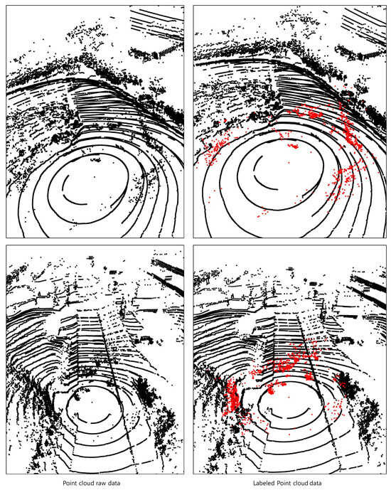
Figure 1.
The result of labeling point cloud data obtained under adverse weather conditions through experiments. The red points represent those annotated as noise.
3.3. Data Annotation
Let the point cloud set that we captured be , where i denotes the index of the scene of LiDAR scans taken in clean weather conditions at location j. stands for the number of point cloud of the scene i at location j. Since clean weather scenes are assumed to contain no significant noise, as shown in the Figure 2, we can aggregate the points from multiple scenes at location j to estimate the static objects such as building and sidewalk. These points are referred to as static points and defined as follows:
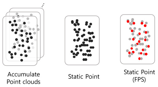
Figure 2.
Static point cloud extraction: accumulate the point cloud over the scenes and extract static point cloud from the accumulated points by applying FPS. Black and red points represent accumulated point cloud and filtered points by FPS, respectively.
, denotes the total number of scenes of location j captured in clean weather and the lidar point, respectively. Points within a certain range of each accumulated point across different scenes are considered to belong to the same cluster. By analyzing the number of scenes in which the points within each cluster appear, we filter out moving objects and temporarily static objects that only exist in a limited number of scenes, such as parked vehicles. This process allows us to distinguish the static points from the dataset captured from each location.
Using these extracted static points, we measure the distance of points in adverse weather scenes. If the distance exceeds a certain threshold, the point is defined as a noise point. However, since static points are derived from point clouds accumulated over numerous scenes, such computations are expensive and involve substantial computational overhead. To improve efficiency while still accurately defining the boundary points of static point clusters, following prior works [26,41,42], we applied farthest-point sampling (FPS) [43] to select representative points.
To subsample representative points from a large-scale accumulated point cloud, FPS is commonly employed. FPS sequentially selects the points such that each maximizes the minimum distance to the previously selected points . This procedure effectively distributes the sampled points to maximize spatial coverage within the metric space. Through this process, a well-distributed representative subset can be effectively selected from the static points, significantly reducing the overall computational cost. Through iterative experimental validation, the 1/3 sampling ratio with a threshold distance of 0.3 m was determined to achieve optimal balance between computational efficiency and information preservation.
Under adverse weather conditions, we compute the distance from each point in the observed point cloud to the FPS-sampled static points. Points beyond the threshold are labeled as noise. In some frames, moving objects, such as vehicles or pedestrians, may still appear. To reduce false positives, we incorporate an object detection network to filter out dynamic objects as a first-stage refinement. In the second stage, we leverage camera imagery for additional label correction and refinement.
4. Methodology
Unlike indoor scenes with relatively dense point distributions, point clouds in autonomous driving scenarios are inherently sparse due to open environments. Although nearby objects are captured with high point density, distant objects often lack sufficient points, making it difficult to perceive the surrounding space accurately. Under adverse weather conditions, the presence of noise among these already sparse points further exacerbates the problem. To address these challenges, we propose SCOPE (Context-Aware Point Cloud Encoder), a model designed to classify noise points within LiDAR point clouds under adverse weather conditions. SCOPE partitions the 3D space into uniformly sized voxels and extracts features from the points within each voxel to classify noise points. To accomplish this effectively, we introduce spatial attentive pooling, which captures the geometric relationships among points within a voxel. Furthermore, we apply contrastive learning to ensure that points sharing the same label are embedded into similar clusters. In this section, we present the overall architecture of SCOPE, followed by details on network optimization and training protocols. Figure 3 below shows the overall pipeline of the network proposed in this paper.
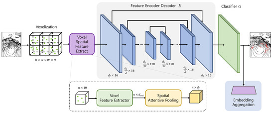
Figure 3.
Overview of the proposed denoising model, SCOPE. Our network is structured into three core components: the Voxel Spatial Feature Extractor (VSFE), a Feature Encoder–Decoder, and a Classifier Layer. The VSFE module includes two key stages: the Voxel Feature Extractor (VFE) and Spatial Attentive Pooling (SAP). The VFE enriches the geometric attributes of input points and extracts features from the enhanced representations. The SAP layer then learns to aggregate spatial features and geometric patterns by focusing on the K nearest neighboring points.
4.1. Problem Formulation
The Figure 4 illustrates the VFE proposed in this paper. Let the source domain be defined as , where denotes a LiDAR point cloud scan and represents its corresponding point-wise semantic annotations. The objective is to train a 3D point cloud segmentation model capable of accurately identifying and classifying noise points induced by adverse weather conditions. To achieve this, we construct a voxelized representation of the point cloud, where each voxel aggregates semantic features derived from the points residing within its spatial bounds. The segmentation model is composed of a feature extractor followed by a classifier , such that . This formulation enables the model to leverage local semantic structures while remaining robust to weather-induced noise artifacts.
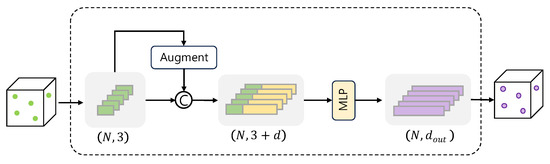
Figure 4.
Illustration of the Voxel Feature Extractor (VFE), which enhances the geometric fidelity of input points by embedding enriched spatial descriptors and subsequently extracts high-level feature representations from the augmented point set.
4.2. Voxel Feature Extractor
Voxelization provides a structured and computationally tractable approach to organizing raw 3D point cloud data by discretizing the continuous spatial domain into a regular grid of uniformly sized volumetric elements, or voxels. Each voxel serves as a localized container for aggregating geometric and semantic information from the points falling within its bounds, enabling efficient parallel processing and preserving spatial locality.
To initialize voxel-wise feature computation, the raw points contained within each voxel are first aggregated. However, given the limited descriptive power of raw spatial coordinates alone—especially in sparse or noisy environments—each point is enriched with a set of informative geometric descriptors to enhance feature expressiveness. Specifically, each point is augmented with a 10-dimensional feature vector , defined as
where are the global 3D coordinates of the point p, and r denotes its reflectance value. The triplet encodes the offset of the point from the mean (centroid) of all points within the same voxel, capturing local geometric context. Meanwhile, represents the point’s relative displacement from the geometric center of the voxel, providing positional awareness within the voxel grid.
This augmented feature vector is then passed through a lightweight Multi-Layer Perceptron (MLP) to transform the raw input into a more discriminative representation. The MLP consists of a linear projection layer, followed by Batch Normalization and a ReLU activation function, facilitating stable training and non-linear feature encoding. This transformation yields rich voxel-wise features that form the foundation for subsequent spatial reasoning and semantic inference.
4.3. Spatial Attentive Pooling
The Spatial Attentive Pooling (SAP) layer is a pivotal module in our proposed framework, meticulously designed to enhance the encoding and aggregation of localized spatial features within each voxel. By concurrently capturing both intra-voxel spatial configurations and inter-point geometric relationships, the SAP layer empowers the network to develop a richer and more structured understanding of the underlying 3D space. This enables the generation of highly discriminative point-wise features, which are particularly critical for robust performance under sparse and noisy point cloud conditions. The overall architecture of the SAP layer is illustrated in Figure 5.

Figure 5.
The Spatial Attentive Pooling units learn to aggregate geometric patterns and features from the K nearest neighboring points, ultimately producing a rich and informative feature representation.
Starting from voxel-level feature extraction, each point within a voxel is embedded with a feature vector that reflects its relative spatial configuration. For a given center point feature and its K nearest neighbors , we explicitly encode local geometric context using a feature mixing strategy formulated as
where ⊕ denotes vector concatenation, and captures the pairwise geometric offset between the center point and its k-th neighbor. The multi-layer perceptron (MLP) is applied to learn local geometric patterns by assigning weights that capture the importance of these relative relations and representative feature inside the voxel.
To selectively emphasize informative local features, we apply an attention mechanism that assigns importance weights to the neighboring features. Specifically, attention scores are derived via a fully connected layer followed by softmax normalization:
where denotes the attention coefficient for the k-th neighbor, ⊙ indicates element-wise multiplication, and is the resulting aggregated feature for the center point. This attention-guided aggregation ensures that more informative and geometrically significant neighbors exert greater influence on the final representation.
To preserve the original spatial structure and mitigate overfitting, we incorporate a residual connection that combines the attentively pooled feature with a learned transformation of the original input. The final output of the SAP layer is given by
where the max operation is applied across feature channels to enhance robustness, and the concatenation with a transformed neighbor feature ensures that both local refinement and raw structural cues are retained in the final voxel-wise representation.
Through this carefully designed attention-based pooling strategy, the SAP layer serves as a powerful mechanism to capture intricate spatial dependencies, even under sparse and noisy conditions, which are characteristic of real-world LiDAR point clouds in autonomous driving scenarios.
4.4. Embedding Aggregation
To robustly distinguish between valid points and noise points (e.g., those caused by fog or snow) in adverse weather conditions, we adopt a contrastive learning strategy during the training phase. After extracting representative feature vectors f from each voxel, we encourage the network to learn a latent space where features from the same semantic group (i.e., either noise or valid) are pulled closer together, while those from different groups are pushed farther apart. This promotes intra-class compactness and inter-class separability in the feature space, facilitating more reliable segmentation under noisy environments. The contrastive loss is formulated as
where denotes the feature embedding of the i-th voxel obtained from the SAP module, and indicates the set of indices within the same batch that share the same class label with . Conversely, represents the set of indices corresponding to different class labels. The temperature parameter controls the sharpness of the similarity distribution. This formulation encourages feature embeddings of voxels belonging to the same class to be pulled closer, while pushing apart those from different classes. Consequently, the network learns discriminative and compact clusters for each label, thereby improving segmentation robustness under noisy conditions. where N is the number of voxels in the batch, is a temperature parameter, and · denotes the inner product between normalized embeddings.
Through the network’s classifier G, point-wise prediction for each input point cloud are generated, and by comparing these with the actual ground truth, the cross-entropy loss is induced. By integrating the supervised cross-entropy loss with the contrastive learning loss, the overall training loss is formulated as follows:
5. Experiments
5.1. Data Construction
To evaluate the effectiveness of the proposed network in identifying noise points in adverse weather conditions, we utilize the dataset we collected using a LiDAR-equipped experimental vehicle under clean and adverse weather conditions. The dataset was constructed by labeling noise points under adverse weather conditions based on points acquired in clean weather, resulting in two labels: valid and noise. 80% of the data is used as the training set for training the network proposed in this study, and the remaining 20% is used as the test set. Each point in the adverse-weather LiDAR scan was labeled as either noise (1) or valid (0). This labeling process resulted in a binary segmentation task where the goal is to distinguish noise from valid points in point cloud data obtained under challenging weather conditions.
5.2. Implementation Details
To ensure consistent spatial density across varying LiDAR scan qualities, we downsample raw LiDAR point clouds using voxel grid filtering. Specifically, we retain a single representative point within each voxel of size 10 cm × 10 cm × 10 cm. This preprocessing step reduces redundancy in dense regions while preserving the geometric structure of the scene. Following downsampling, we project the point cloud onto a discretized 3D grid. The spatial dimensions along the X, Y, and Z axes are divided into bins, respectively. These discretized grids are used to extract localized context while maintaining a compact representation of the overall scene. For local neighborhood feature aggregation, we use the K nearest neighbors algorithm with .
We optimize our network using the AdamW optimizer [44], which combines the benefits of adaptive learning rates and decoupled weight decay. The training is conducted for a total of 20 epochs. The weight decay coefficient is fixed at 0.005 to regularize the model and prevent overfitting. We employ a two-stage learning rate scheduling strategy: for the first 2 epochs, we apply a linear warm-up that linearly increases the learning rate from 0 to 0.01. After the warm-up, the learning rate decays by a factor of 0.95 after each epoch, allowing stable convergence as training progresses.
Each training batch contains four samples per GPU. To improve the robustness of the model against sensor noise, spatial variance, and environmental changes, we employ a suite of data augmentation techniques. These include:
- Random Rotation: applied around the Z-axis to simulate changes in heading direction.
- Anisotropic Scaling: independent scaling along each axis to emulate distortions from LiDAR sensor calibration drift.
- Random Flipping: performed along the XY-plane to introduce further diversity in spatial configurations.
Additionally, we apply stochastic depth regularization during training to improve generalization in deeper architectures. A layer drop probability of 0.2 is used, meaning each residual layer has a 20% chance of being skipped during training iterations.
The overall loss function comprises three complementary components: cross-entropy loss, softmax loss.
All experiments are conducted on a workstation running Ubuntu 18.04, equipped with two NVIDIA RTX 4090 GPUs and 24 GB of system memory. The implementation is based on PyTorch 4.50, with distributed data parallel training enabled for multi-GPU scalability. Checkpoints are saved at every epoch, and the best-performing model on the validation set is selected for final evaluation.
5.3. Evaluation Metrics
Following prior works [45,46], we quantitatively assess the effectiveness of our point cloud denoising approach using four standard evaluation metrics: precision, recall, F1 Score, and Mean Intersection over Union (mIoU). These metrics provide a comprehensive view of the model’s ability to correctly distinguish noise from valid LiDAR points. Precision quantifies the proportion of points predicted as noise that are actually noise, while recall measures the proportion of true noise points that the model successfully identifies. These are formally defined as
where (true positives) denotes the number of noise points correctly identified, (false positives) indicates non-noise points mistakenly labeled as noise, and (false negatives) represents noise points that the model failed to detect.
The F1 Score is the harmonic mean of precision and recall, offering a balanced metric that is particularly useful when the dataset is imbalanced:
mIoU evaluates the overlap between predicted and ground-truth noise point sets, normalized by their union. This metric is widely used in semantic segmentation tasks and is defined as
Together, these metrics provide a thorough evaluation framework for measuring the denoising accuracy and robustness of our proposed method across various noise conditions.
6. Results
6.1. Qualitative Results
In this study, we conduct a series of experiments under three distinct adverse weather conditions: fog, snow, and rain. The experimental results corresponding to snow and rain conditions are illustrated in Figure 6 and Figure 7, respectively. The red points denote those that are correctly identified as noise, while the blue points represent false predictions. Specifically, these include cases where noise points are incorrectly recognized as valid, or valid points are mistakenly classified as noise. It is important to note that the data used for snow and rain scenarios were collected under moderate weather—neither heavy snowfall nor torrential rainfall was present during data acquisition. Under such moderate conditions, LiDAR returns from snow and rain particles appear visually similar, making it difficult to differentiate between them based solely on point cloud representations.
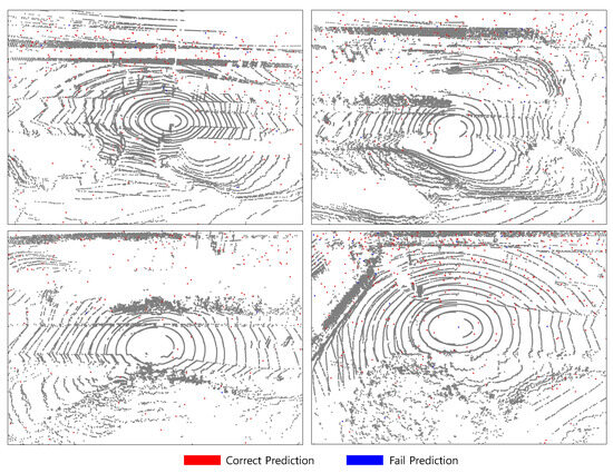
Figure 6.
Qualitative analysis on our dataset in the case of rain.
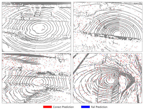
Figure 7.
Qualitative analysis on our dataset in the case of snow.
In both light snowfall and light rain conditions, the individual precipitation particles exhibit relatively small physical dimensions and are dispersed sparsely throughout the atmosphere. Due to their limited size and low spatial density, these particles exert minimal interference with the LiDAR sensor’s line of sight. As a result, they are less likely to cause significant occlusion of objects within the scene or to form coherent or dense clusters within the resulting point cloud. Instead, such precipitation typically manifests as a sparse set of isolated points that are spatially detached from solid surfaces and object boundaries. These atmospheric points can be effectively identified and filtered as noise due to their characteristic spatial and temporal properties—namely, their lack of structural continuity and inconsistency across consecutive frames. Importantly, the presence of these sparse noise points does not substantially distort the underlying geometric structure of nearby objects, preserving the integrity of object boundaries and scene topology. This characteristic leads to a relatively lower complexity for perception tasks such as segmentation or detection under these specific non-clear weather conditions, in contrast to more adverse weather scenarios. Consequently, scene understanding remains tractable in light snowfall and light rain, supporting the robustness of LiDAR-based perception systems under mild environmental disturbances.
However, in adverse weather conditions such as heavy snowstorms or intense rainfall, the concentration of atmospheric particles increases dramatically, resulting in frequent occlusions and spurious reflections in LiDAR signals. These effects can substantially degrade the quality of point cloud data, leading to reduced model performance. Therefore, to accurately assess model robustness in real-world deployments, it is crucial to include experiments with data collected under such extreme environmental conditions.
Figure 8 presents the experimental results under foggy conditions. In contrast to snow or rain, fog consists of much finer particles that are densely distributed throughout the atmosphere. These particles are highly effective at scattering LiDAR beams, which can severely impact sensing performance. In cases of dense fog, the maximum effective sensing range of the LiDAR can be substantially reduced, posing serious challenges for downstream perception tasks.
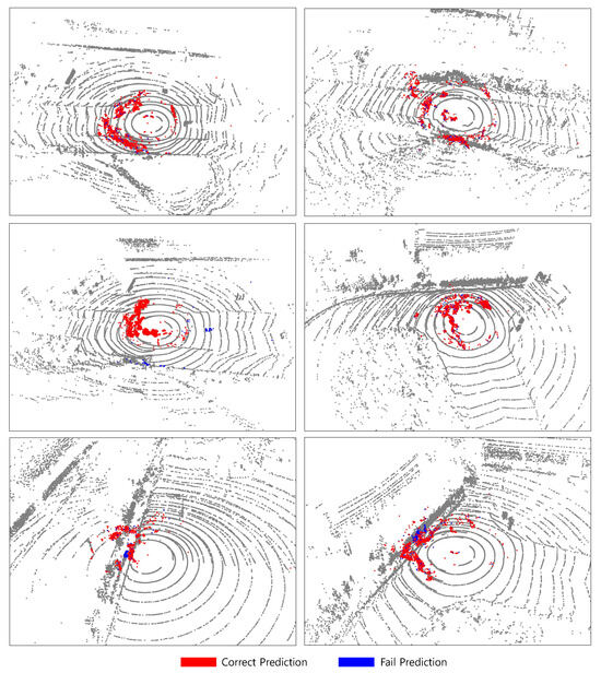
Figure 8.
Qualitative analysis on our dataset in the case of fog. In the case of fog, it can be divided into dense fog (top) and relatively lighter fog (bottom). In dense fog, water particles suspended in the air are densely packed, creating a barrier-like shape as seen in the image.
Moreover, dense fog not only attenuates the LiDAR signal, but also induces the formation of high-density particle clusters around the sensor, distorting object shapes. In our observations, heavy fog often causes LiDAR returns to form thick, wall-like structures encircling the sensor. These fog-induced pseudo-clusters are especially problematic when overlapping with real objects. As shown in the bottom row of Figure 8, such clusters near vegetation often lead to misclassification, with parts of vegetation mislabeled as noise, or vice versa.
Furthermore, occlusion caused by dense fog can significantly degrade downstream object detection performance. Partial visibility or spurious points can lead to missed detections or inaccurate bounding boxes, particularly in safety-critical scenarios. Our experiments confirm that under severe fog, detection confidence and localization accuracy are notably reduced.
Despite these challenges, our method demonstrates effective discrimination of noise points in most scenarios. We attribute this robustness to two key design choices: (1) the vehicle operated within a constrained spatial region during data acquisition, thereby reducing environmental variability, and (2) the dataset was annotated with only two semantic categories—valid points and noise points—which simplifies the segmentation task and enhances classification clarity under adverse weather conditions.
6.2. Quantitative Results
We conducted a comprehensive evaluation of our method using standard binary classification metrics: precision, recall, F1-score, and Intersection over Union (IoU) for the noise class across diverse adverse weather scenarios, namely snow, rain, and fog. We compare our method with state-of-the-art models spanning both statistical techniques and deep learning architectures. In particular, DROR [47] represents a statistical baseline, while SalsaNext [48], originally designed for general point cloud segmentation, has been adapted to a binary classification setting to facilitate fair comparison. Additionally, we include specialized point cloud denoising networks such as WeatherNet [49] and 4DenoiseNet [50] in our comparative analysis.
Table 1 presents a detailed quantitative comparison of adverse weather noise point classification performance under adverse weather conditions on our newly proposed dataset. We evaluate the models using standard metrics: precision, recall, F1 score, and mean Intersection over Union (mIoU). As shown in Table 1, our approach demonstrates the highest mIoU across all three challenging scenarios—snow, rain, and fog—outperforming recent state-of-the-art denoising models such as 4DenoiseNet and WeatherNet. Specifically, our method surpasses SalsaNet by 1.05%, 5.73% and 3.95% mIoU under the snow, rain and fog scenarios, respectively, 4DenoiseNet by 3.84%, 7.51%and 5.54% mIoU in snow, rain and fog, respectively. It is also noteworthy that our model achieved the top mIoU scores of 88.66%, 92.33%, and 88.77% for snow, rain, and fog scenarios, respectively. Meanwhile, DROR achieves the highest recall in snow and rain scenarios, and 4DenoiseNet achieves the highest recall in fog scenarios. These results demonstrate the robustness and generalizability of our method for weather-induced noise point classification on our dataset, highlighting its effectiveness across diverse and challenging environmental conditions.

Table 1.
Adverse weather noise classification performance results on the our proposed weather datasets. P, R denote precision and recall, respectively. Bold font indicates the best performance within each column.
Quantitatively, in the rain scenario, our model achieved the highest scores across all metrics except recall. DROR achieved the highest recall of 97.52 in this scenario. However, its relatively low precision indicates that DROR tends to classify most points as clear, resulting in a lower proportion of correctly identified noise points.
Unlike severe snowstorms or heavy fog, the rain points under the moderate condition do not occlude object surfaces or cause significant geometric distortion. They are sparsely distributed on the air, without heavily overlapping with foreground structures. As a result, these points are less likely to interfere with the underlying object geometry, making it easier for the network to detect and segment them accurately.
In the snow scenario, our method achieved the highest scores across all metrics, except for recall, where DROR obtained the best result with a recall of 95.24—similar to the trend observed in the rain scenario. Notably, our method showed only a marginal difference in performance compared to SalsaNet. Unlike rain, snow can distort object shapes in the point cloud, which likely led to a slightly lower mIoU than that achieved under rain conditions.
This phenomenon is particularly severe in the fog scenario, where all models, including ours, achieved the lowest mIoU. Dense fog increases the density of airborne noise points, severely occluding the scene and distorting object geometry. Furthermore, as shown in Figure 8, when the shape of the fog overlaps with surrounding objects, it becomes even more challenging for the network to correctly classify points. Therefore, it is crucial for the model to effectively capture both the local features and the geometrical relationships among points, enabling it to learn and recognize the unique geometric patterns induced by fog.
It is also important to note that the data collection and annotation strategy used in this study may have contributed to the overall strong performance. Since point cloud data were collected under adverse weather with limited scenarios, the dataset includes limited set of locations and scene types. Many of the test scenes share similar environmental structures, background geometry, and object distributions. This scene-level redundancy could have aided the model’s learning and generalization within the domain, thereby slightly inflating performance metrics. To address this limitation, future work should expand the dataset to include more diverse scenarios with various object classes and scenarios.
6.3. Ablation Study
The encoder ingests the raw LiDAR point attributes x, y, z, along with the center position of each voxel and the relative distance from the center. By encoding these relative distances within the local coordinate system of each voxel, the model achieves invariance to an absolute position and effectively normalizes the local spatial context. This point-level augmentation facilitates learning the geometric relationships among points within a voxel. The effectiveness of this augmentation strategy and the contrastive learning are quantitatively validated in Table 2. It shows that introducing contrastive learning improves mIoU by 0.3–0.8% across all scenarios.
Table 2.
Ablations study for encoder point augmentations in voxel feature extract and the adaptation of the contrastive learning loss. A check mark indicates that the corresponding item has been applied.
In spatial attentive pooling, we aggregate features from K neighboring points. The effect of varying K on performance is summarized in Table 3. As K increases, the model benefits from richer cross-referenced contextual information, leading to an overall improvement in performance. However, when K reaches 32, the performance gain saturates and in some cases slightly degrades. Additionally, larger values of K incur higher computational costs. Based on this trade-off, we set K to 16 as the overall F1 score is highest.
Table 3.
Ablations study for the number of the neighboring point K. Bold font indicates the best performance within each column.
7. Conclusions
Under adverse weather conditions, the information in LiDAR point clouds is often distorted or lost due to a large number of noise points. In such challenging environments, it is crucial to accurately capture the feature characteristics of valid points based on the traits of airborne noise particles, and to understand the spatial context among points to enable correct point classification. However, annotating noise points in adverse weather conditions is a very difficult and time-consuming task. To address this, simulation models or synthetic data have often been proposed as alternatives, but there are still some differences compared to naturally obtained data. In this study, we developed an effective data acqusition strategy, which is capturing corresponding scenes under both adverse and clear weather and comparing them to identify and label noise points, thereby ensuring high-quality annotations.
In this work, we proposed a novel network, SCOPE, designed to perform robust point cloud segmentation under adverse weather conditions. Under such conditions, LiDAR data is often severely corrupted due to the presence of airborne noise particles, which distort the spatial distribution of valid points and hinder accurate scene understanding. To tackle this, SCOPE effectively models the spatial context among points and learns to increase the separation in vector space between noise and valid points. This enables the network to capture subtle but critical differences in point characteristics and improves its ability to distinguish true object surfaces from noise.
Our experimental results show that the proposed method achieves a mean Intersection over Union (mIoU) of 88.66%, 92.33%, and 88.77% across the snow, rain, and fog scenarios, respectively. These results validate the effectiveness of our approach in practical scenarios where clean and noisy data distributions diverge significantly.
However, the dataset used in this study was collected from a limited set of locations and scenarios, which led to a degree of scene repetition and structural similarity across the samples, while this helped stabilize training and may have contributed to high performance within the domain, it also introduces a potential limitation in terms of generalization to unseen environments. To address this, future work should focus on expanding the dataset to include more diverse scenes such as heavy snow or heavy rain, object categories, and dynamic conditions, which will be essential for further improving the robustness and applicability of noise-resilient perception models in real-world autonomous systems.
Funding
This work was supported by an Incheon National University Research Grant in 2025.
Institutional Review Board Statement
Not applicable.
Informed Consent Statement
Not applicable.
Data Availability Statement
The original contributions presented in the study are included in the article, further inquiries can be directed to the corresponding author.
Conflicts of Interest
The authors declare no conflicts of interest.
References
- Tang, J.; Tian, F.-P.; Feng, W.; Li, J.; Tan, P. Learning guided convolutional network for depth completion. IEEE Trans. Image Process. 2021, 30, 1116–1129. [Google Scholar] [CrossRef]
- Gao, Y.; Li, W.; Wang, J.; Zhang, M.; Tao, R. Relationship learning from multisource images via spatial-spectral perception network. IEEE Trans. Image Process. 2024, 33, 3271–3284. [Google Scholar] [CrossRef]
- Zhang, Y.; Carballo, A.; Yang, H.; Takeda, K. Perception and sensing for autonomous vehicles under adverse weather conditions: A survey. ISPRS J. Photogramm. Remote. Sens. 2023, 196, 146–177. [Google Scholar] [CrossRef]
- Zhao, X.; Wen, C.; Prakhya, S.M.; Yin, H.; Zhou, R.; Sun, Y.; Xu, J.; Bai, H.; Wang, Y. Multi-modal features and accurate place recognition with robust optimization for lidar-visual-inertial slam. IEEE Trans. Instrum. Meas. 2024, 73, 1–14. [Google Scholar]
- Eisl, N.; Halperin, D. Point cloud based scene segmentation: A survey. Comput. Graph. Forum 2024, 43, e14234. [Google Scholar]
- Park, J.; Kim, C.; Jo, K. PCSCNet: Fast 3D semantic segmentation of LiDAR point cloud for autonomous car using point convolution and sparse convolution network. Eng. Appl. Artif. Intell. 2022, 113, 104983. [Google Scholar]
- Montalvo, J.; Carballeira, P.; García-Martín, A. SynthmanticLiDAR: A synthetic dataset for semantic segmentation on LiDAR imaging. Comput. Vis. Image Underst. 2024, 239, 103897. [Google Scholar]
- Godfrey, J.; Kumar, V.; Subramanian, S.C. Evaluation of flash lidar in adverse weather conditions towards active road vehicle safety. IEEE Sens. J. 2023, 23, 17234–17242. [Google Scholar] [CrossRef]
- Sezgin, F.; Vriesman, D.; Steinhauser, D.; Lugner, R.; Brandmeier, T. Safe autonomous driving in adverse weather: Sensor evaluation and performance monitoring. In Proceedings of the 2023 IEEE Intelligent Vehicles Symposium (IV), Anchorage, AK, USA, 4–7 June 2023; pp. 1–6. [Google Scholar]
- Li, S.; Wang, Z.; Juefei-Xu, F.; Guo, Q.; Li, X.; Ma, L. Common corruption robustness of point cloud detectors: Benchmark and enhancement. IEEE Trans. Multimed. 2023, 25, 8520–8532. [Google Scholar]
- Vattem, T.; Sebastian, G.; Lukic, L. Rethinking lidar object detection in adverse weather conditions. In Proceedings of the 2022 International Conference on Robotics and Automation (ICRA), Philadelphia, PA, USA, 23–27 May 2022; pp. 5093–5099. [Google Scholar]
- Wang, J.; Wu, Z.; Liang, Y.; Tang, J.; Chen, H. Perception methods for adverse weather based on vehicle infrastructure cooperation system: A review. Sensors 2024, 24, 374. [Google Scholar] [CrossRef] [PubMed]
- Xiao, A.; Huang, J.; Xuan, W.; Ren, R.; Liu, K.; Guan, D.; Saddik, A.E.; Lu, S.; Xing, E.P. 3d semantic segmentation in the wild: Learning generalized models for adverse-condition point clouds. In Proceedings of the IEEE/CVF Conference on Computer Vision and Pattern Recognition (CVPR), Vancouver, BC, Canada, 17–24 June 2023; pp. 9382–9392. [Google Scholar]
- Teufel, S.; Volk, G.; Bernuth, A.V.; Bringmann, O. Simulating realistic rain, snow, and fog variations for comprehensive performance characterization of lidar perception. In Proceedings of the IEEE 95th Vehicular Technology Conference (VTC2022-Spring), Helsinki, Finland, 19–22 June 2022; pp. 1–7. [Google Scholar]
- Xie, Y.; Tian, J.; Zhu, X.X. Linking points with labels in 3D: A review of point cloud semantic segmentation. IEEE Geosci. Remote. Sens. Mag. 2020, 8, 38–59. [Google Scholar] [CrossRef]
- Sarker, S.; Rana, M.M.; Hasan, M.N. A comprehensive overview of deep learning techniques for 3D point cloud classification and semantic segmentation. Mach. Learn. Appl. 2022, 9, 100362. [Google Scholar] [CrossRef]
- Hegde, S.; Gangisetty, S. PIG-Net: Inception based deep learning architecture for 3D point cloud segmentation. IEEE Access 2021, 9, 107771–107781. [Google Scholar] [CrossRef]
- Hahner, M.; Sakaridis, C.; Dai, D.; Gool, L.V. Fog simulation on real LiDAR point clouds for 3D object detection in adverse weather. In Proceedings of the IEEE/CVF International Conference on Computer Vision (ICCV), Montreal, QC, Canada, 10–17 October 2021; pp. 15283–15292. [Google Scholar]
- Lee, J.; Kim, S.; Park, H.; Lee, Y. GAN-based LiDAR translation between sunny and adverse weather conditions for autonomous driving. Sensors 2022, 22, 5287. [Google Scholar] [CrossRef]
- Kim, I.I.; McArthur, B.; Korevaar, E.J. Comparison of laser beam propagation at 785 nm and 1550 nm in fog and haze for optical wireless communications. SPIE 2001, 4214, 26–37. [Google Scholar]
- Rasshofer, R.H.; Spies, M.; Spies, H. Influences of weather phenomena on automotive laser radar systems. Adv. Radio Sci. 2011, 9, 49–60. [Google Scholar] [CrossRef]
- Park, J.; Jang, J.; Kim, Y.; Jo, K. No thing, nothing: Highlighting safety-critical classes for robust LiDAR semantic segmentation in adverse weather. In Proceedings of the IEEE/CVF Conference on Computer Vision and Pattern Recognition (CVPR), Seattle, WA, USA, 16–22 June 2024; pp. 12345–12354. [Google Scholar]
- Yang, H.; Wang, S.; Liu, Z.; Chen, C. Rethinking range-view LiDAR segmentation in adverse weather. IEEE Trans. Pattern Anal. Mach. Intell. 2024, 46, 5432–5447. [Google Scholar]
- Chae, H.; Lee, C.; Park, S.; Kim, J. Towards robust 3D object detection with LiDAR and 4D radar. In Proceedings of the IEEE/CVF Conference on Computer Vision and Pattern Recognition (CVPR), Seattle, WA, USA, 16–22 June 2024; pp. 8765–8774. [Google Scholar]
- Carballo, A.; Lambert, J.; Monrroy, A.; Wong, D.; Narksri, P.; Kitsukawa, Y.; Takeuchi, A.; Kato, S.; Takeda, K. LIBRE: The multiple 3D LiDAR dataset. In Proceedings of the 2020 IEEE Intelligent Vehicles Symposium (IV), Las Vegas, NV, USA, 19 October–13 November 2020; pp. 1094–1101. [Google Scholar]
- Qi, C.R.; Yi, L.; Su, H.; Guibas, L.J. PointNet++: Deep hierarchical feature learning on point sets in a metric space. Adv. Neural Inf. Process. Syst. (Neurips) 2017, 30, 5099–5108. [Google Scholar]
- Qi, C.R.; Su, H.; Mo, K.; Guibas, L.J. PointNet: Deep learning on point sets for 3D classification and segmentation. In Proceedings of the IEEE Conference on Computer Vision and Pattern Recognition (CVPR), Honolulu, HI, USA, 21–26 July 2017; pp. 652–660. [Google Scholar]
- Miao, Y.; Zhang, L.; Wang, Q.; Chen, H. An efficient point cloud semantic segmentation network based on multiscale super-patch transformer. Sci. Rep. 2024, 14, 4567. [Google Scholar] [CrossRef]
- Chen, Z.; Xu, W.; Zhang, X.; Liu, Y. PointDC: Unsupervised semantic segmentation of 3D point clouds via cross-modal distillation and super-voxel clustering. In Proceedings of the IEEE/CVF International Conference on Computer Vision (ICCV), Paris, France, 2–3 October 2023; pp. 8432–8441. [Google Scholar]
- Thomas, H.; Qi, C.R.; Deschaud, J.-E.; Marcotegui, B.; Goulette, F.; Guibas, L.J. KPConv: Flexible and deformable convolution for point clouds. In Proceedings of the IEEE/CVF International Conference on Computer Vision (ICCV), Seoul, Republic of Korea, 27 October–2 November 2019; pp. 6411–6420. [Google Scholar]
- Yan; Xu, C.; Cui, Z.; Zong, Y.; Yang, J. STPC: Spatially Transformed Point Convolution for 3D Point Cloud Learning. In Proceedings of the IEEE/CVF Conference on Computer Vision and Pattern Recognition (CVPR), Seattle, WA, USA, 13–19 June 2020. [Google Scholar]
- Wu, B.; Wan, A.; Yue, X.; Keutzer, K. SqueezeSeg: Convolutional neural networks with recurrent CRF for real-time road-object segmentation from 3D LiDAR point cloud. In Proceedings of the 2018 IEEE International Conference on Robotics and Automation (ICRA), Brisbane, Australia, 21–25 May 2018; pp. 1887–1893. [Google Scholar]
- Zhang, Y.; Zhou, Z.; David, P.; Yue, X.; Xi, Z.; Gong, B.; Foroosh, H. PolarNet: An improved grid representation for online LiDAR point clouds semantic segmentation. In Proceedings of the IEEE Conference on Computer Vision and Pattern Recognition (CVPR), Seattle, WA, USA, 13–19 June 2020; pp. 9601–9610. [Google Scholar]
- Xu, C.; Wu, B.; Wang, Z.; Zhan, W.; Vajda, P.; Keutzer, K.; Tomizuka, M. Spatially Adaptive Convolution for Efficient 3D Point Cloud Segmentation. In Proceedings of the IEEE/CVF Conference on Computer Vision and Pattern Recognition (CVPR), Seattle, WA, USA, 13–19 June 2020. [Google Scholar]
- Wang, L.; Huang, Y.; Hou, Y.; Zhang, S.; Shan, J. Graph Attention Convolution for Point Cloud Semantic Segmentation. In Proceedings of the IEEE Conference on Computer Vision and Pattern Recognition (CVPR), Long Beach, CA, USA, 15–20 June 2019. [Google Scholar]
- Wang, L.; Xu, C.; Zhao, Y.; Zhang, M. UniPre3D: Unified pre-training of 3D point cloud models with cross-modal fusion. In Proceedings of the IEEE/CVF Conference on Computer Vision and Pattern Recognition (CVPR), Seattle, WA, USA, 16–22 June 2024; pp. 15678–15687. [Google Scholar]
- Lin, H.; Chen, S.; Wang, M.; Liu, J. HiLoTs: High-low temporal sensitive representation learning for semi-supervised LiDAR segmentation. In Proceedings of the IEEE/CVF Conference on Computer Vision and Pattern Recognition (CVPR), Seattle, WA, USA, 16–22 June 2024; pp. 18234–18243. [Google Scholar]
- Choy, C.; Gwak, J.; Savarese, S. 4D spatio-temporal ConvNets: Minkowski convolutional neural networks. In Proceedings of the IEEE Conference on Computer Vision and Pattern Recognition (CVPR), Long Beach, CA, USA, 15–20 June 2019; pp. 3075–3084. [Google Scholar]
- Liu, Z.; Tang, H.; Zhao, S.; Shao, K.; Han, S. Point-Voxel Neural Architecture Search for 3D Deep Learning. In Proceedings of the IEEE Conference on Computer Vision and Pattern Recognition (CVPR), Nashville, TN, USA, 20–25 June 2021. [Google Scholar]
- Zhu, X.; Zhou, H.; Wang, T.; Hong, F.; Ma, Y.; Li, W.; Li, H.; Lin, D. Cylindrical and asymmetrical 3D convolution networks for LiDAR segmentation. In Proceedings of the IEEE Conference on Computer Vision and Pattern Recognition (CVPR), Nashville, TN, USA, 20–25 June 2021; pp. 9939–9948. [Google Scholar]
- Li, Y.; Bu, R.; Sun, M.; Wu, W.; Di, X.; Chen, B. PointCNN: Convolution on X-transformed points. In Proceedings of the Advances in Neural Information Processing Systems (NeurIPS), Vancouver, BC, Canada, 8–14 December 2019; pp. 820–830. [Google Scholar]
- Wu, W.; Qi, Z.; Fuxin, L. PointConv: Deep convolutional networks on 3D point clouds. In Proceedings of the IEEE Conference on Computer Vision and Pattern Recognition (CVPR), Long Beach, CA, USA, 15–20 June 2019; pp. 9621–9630. [Google Scholar]
- Eldar, Y.; Lindenbaum, M.; Porat, M.; Zeevi, Y.Y. The farthest point strategy for progressive image sampling. IEEE Trans. Image Process. 1997, 6, 1305–1315. [Google Scholar] [CrossRef] [PubMed]
- Kingma, D.P.; Ba, J. Adam: A method for stochastic optimization. In Proceedings of the International Conference on Learning Representations (ICLR), San Diego, CA, USA, 7–9 May 2015. [Google Scholar]
- Zhao, X.; Wen, C.; Wang, Y.; Bai, H.; Dou, W. TripleMixer: A 3D point cloud denoising model for adverse weather. arXiv 2024, arXiv:2408.13802. [Google Scholar] [CrossRef]
- Raisuddin, A.M.; Cortinhal, T.; Holmblad, J.; Aksoy, E.E. Learning to denoise raw mobile LiDAR data for robust localization. In Proceedings of the IEEE Intelligent Vehicles Symposium (IV), Jeju Island, Republic of Korea, 2–5 June 2024; pp. 2862–2868. [Google Scholar]
- Charron, N.; Phillips, S.; Waslander, S.L. De-noising of lidar point clouds corrupted by snowfall. In Proceedings of the 2018 15th Conference on Computer and Robot Vision (CRV), Toronto, ON, Canada, 8–10 May 2018; pp. 254–261. [Google Scholar]
- Cortinhal, T.; Tzelepis, G.; Aksoy, E.E. SalsaNext: Fast, uncertainty-aware semantic segmentation of LiDAR point clouds. In Advances in Visual Computing; Springer: Berlin/Heidelberg, Germany, 2020; pp. 207–222. [Google Scholar]
- Heinzler, R.; Piewak, F.; Schindler, P.; Stork, W. Cnn-based lidar point cloud de-noising in adverse weather. IEEE Robot. Autom. Lett. 2020, 5, 2514–2521. [Google Scholar] [CrossRef]
- Seppänen, A.; Ojala, R.; Tammi, K. 4DenoiseNet: Adverse weather denoising from adjacent point clouds. IEEE Robot. Autom. Lett. 2022, 8, 456–463. [Google Scholar] [CrossRef]
Disclaimer/Publisher’s Note: The statements, opinions and data contained in all publications are solely those of the individual author(s) and contributor(s) and not of MDPI and/or the editor(s). MDPI and/or the editor(s) disclaim responsibility for any injury to people or property resulting from any ideas, methods, instructions or products referred to in the content. |
© 2025 by the author. Licensee MDPI, Basel, Switzerland. This article is an open access article distributed under the terms and conditions of the Creative Commons Attribution (CC BY) license (https://creativecommons.org/licenses/by/4.0/).