Abstract
Understanding the interaction between submerged water jets and cohesive deep-sea sediment is critical for optimizing deep-sea polymetallic nodule hydraulic mining techniques. This research investigated the distinct erosion behavior of cohesive sediments through laboratory experiments and numerical simulations. Cohesive deep-sea sediments were simulated using bentonite–kaolinite mixtures. A series of laboratory experiments, including vane shear tests and viscosity tests under varying moisture content, were conducted to assess the sediments’ mechanical properties. Experimental submerged water jet erosion tests provided basic data for validating the numerical simulations. A Eulerian multi-fluid (EMF) model was implemented to capture sediment–water jet interactions under varying operational parameters, including jet velocities and nozzle heights. The erosion process was found to comprise three distinct stages, including rapid erosion, steady erosion, and stabilization. Two distinct erosion mechanisms were identified, depending on the jet intensity, which affected the depth and shape of the erosion pits. Quantitative analysis revealed that erosion depth exhibits an approximately linear relationship with jet velocity and nozzle height, whereas the erosion diameter shows nonlinear characteristics. These findings enhance the fundamental understanding of cohesive sediment responses under hydraulic disturbances, providing crucial insights for the design and optimization of efficient deep-sea mining systems.
1. Introduction
Deep-sea mineral deposits are rich in metallic resources such as polymetallic nodules, cobalt-rich crusts, and sulfides [1,2,3], and they play a critical role in the global supply of energy and metal resources. How to efficiently and sustainably extract these resources has become one of the key issues in the current development of marine resources. Studies on the mining of polymetallic nodules have focused on improving extraction efficiency and optimizing mining methods [4]. Among these, hydraulic mining, especially water jet technology, has gradually emerged as one of the core techniques in deep-sea mining due to its high efficiency and low cost [5]. Water jet technology operates by directing high-pressure water jets at the sediment surface, utilizing the kinetic energy of the water to disturb and loosen surface sediments [6,7], thereby enabling the uplift and collection of nodule particles [8]. In this process, the water jets must effectively erode the sediment layer and act directly on the target mineral to ensure successful collection. Existing studies tend to oversimplify the interaction between water jets and sediments [9,10], typically assuming that nodule particles lie on a rigid and flat surface and focusing solely on water jet–nodule particle interactions [11,12]. Few studies have thoroughly investigated how the actual presence and specific physical properties of sediments influence the behavior of the water jets. In reality, deep-sea sediments, due to their complex mechanical properties, significantly affect water jet erosion efficiency [13,14]. Parameters such as water jet velocity, water jet angle, and nozzle height [15] cause significantly different erosion behaviors. Therefore, accurately simulating the response characteristics of the sediments and analyzing the changes in erosion performance under water jet action have become essential research topics in the advancement of deep-sea mining technologies.
Unlike a free jet in air, a submerged water jet encounters significant density resistance and viscosity effects immediately upon exiting the nozzle, resulting in more complex flow field structures [16]. Substantial research has been conducted on submerged water jets, primarily focusing on how nozzle geometry influences flow fields [17] and the variation in jet diffusion characteristics [18]. Kartal et al. [19] investigated the effect of annular plates inside circular nozzles and found that the erosion depth of sediment was approximately 70–75% of that observed without the plates. Two years later, the same group examined the jet momentum produced by circular and Venturi nozzles with identical outlet diameters [17]. Other studies explored the diffusion behavior of circular nozzles at varying nozzle heights [18], providing theoretical support for water jet design in underwater operations.
Current research on sediment erosion is largely concentrated on ideal granular media, such as non-cohesive sand beds [20,21]. Experiments have shown that parameters such as jet velocity, jet angle, and nozzle height significantly influence sediment entrainment and particle transport [22]. For instance, Wang et al. [23] found a strong linear relationship between jet velocity and the geometric characteristics of the resulting scour hole in non-cohesive beds. Wang et al. [24] further demonstrated that higher jet velocities significantly enhance sediment suspension and migration. These findings provide valuable insights for erosion studies. However, deep-sea sediments differ considerably from typical sand beds due to their high moisture content, fine particle size, and cohesive nature, resulting in markedly different mechanical behaviors and erosion characteristics [25]. Taştan et al. [26] also confirmed the distinct erosion responses of cohesive versus non-cohesive sediments, observing shallower erosion depths in non-cohesive materials under identical jet conditions. Preliminary studies have been conducted on the erosion of cohesive deep-sea sediment by water jets [27,28], and experimental investigations were also carried out [29]. However, systematic investigations into erosion mechanisms and quantitative parameter relationships remain limited, and a unified analytical framework has not yet been established. Further exploration is thus required to understand how deep-sea sediments respond to water jet-induced disturbances.
To more accurately simulate sediment response to water jets, various numerical methods have been proposed, including smoothed particle hydrodynamics (SPH) [30], arbitrary Lagrangian–Eulerian (ALE) methods [31], and the EMF model [32]. While Lagrangian methods can finely capture individual particle motions, they often face computational bottlenecks when dealing with the significant number of micron-scale particles in deep-sea sediments [32]. In contrast, the EMF model describes fluid–particle and particle–particle interactions at the continuum scale by coupling mass and momentum conservation equations for both phases [33]. Many researchers have successfully applied this model to simulate the erosion of sediments [34,35,36], with experimental validations confirming its physical reliability. The model has been widely used in studies of sediment transport, suspension, and migration, and it has demonstrated considerable accuracy.
Given the aforementioned research background, the erosion mechanisms of deep-sea sediments under the impact of submerged water jets remain poorly understood. Therefore, this study aims to investigate the erosion process of submerged water jets impacting sediments under varying jet velocities and nozzle heights. The research integrates experimental validation with numerical simulation: laboratory experiments are conducted to collect key response data regarding sediment erosion under water jet impact; in parallel, a simulation model is developed based on the EMF method and experimental results to replicate and analyze erosion behavior under different operational conditions. The findings of this study are expected to elucidate the response mechanisms of deep-sea sediments under water jet disturbance, thereby providing a theoretical foundation and technical reference for the structural optimization and parameter design of deep-sea hydraulic mining systems.
2. Materials and Methods
2.1. Numerical Methods
2.1.1. EMF Model Governing Equations
In this study, ANSYS Fluent 19.2 was employed and the EMF method within it was utilized for the numerical simulation analysis. The EMF model can be used to model multiple phases that are mutually independent but interact with each other. In this model, the granular phase is treated as a continuous phase, similar to the primary phase (gas or liquid). All phases share the same pressure, and the volume fraction equation, mass conservation equation, and momentum equation for each phase are solved separately.
The volume fraction of phase is defined by
The mass conservation equation of phase is given by
where is the physical density of phase , is the velocity of phase , represents the mass transfer from phase to phase , and represents the mass transfer from phase to phase .
The momentum conservation equation of phase is given by
where is the stress–strain tensor of phase , defined by
where is the shear viscosity of phase , is the bulk viscosity of phase , is the inter-phase interaction force, is the lift force, is the wall lubrication force, is the virtual mass force, is the turbulent dispersion force, and is the pressure shared by all phases. represents the inter-phase velocity, defined as follows: if (indicating mass transfer from phase to phase ), then ; otherwise, if , then .
Equation (4) must be represented using the appropriate inter-phase interaction force , and for the liquid–solid phase, it is written as . The force is dependent on frictional forces, pressure, cohesion, and other effects. The interaction force is defined in the EMF model using the following form:
where is the momentum exchange coefficient of the liquid and solid phase, is the particle relaxation time, is the particle diameter, and is a function of the drag function () and the relative Reynolds number (). By substituting Equations (6)–(8) into Equation (4), the momentum conservation equations for the liquid–solid (Equation (9)) phases in the EMF model are thus obtained.
In Equation (9), it is necessary to select appropriate forces for the solid phase, such as , , , , and . Since the computational domain of primary interest is situated at a significant distance from the walls, the calculation of can be neglected.
can be derived from the Syamlal–O’Brien model, the Dalla Valle model, and the relative Reynolds number calculation method applicable to the Eulerian multiphase flow particle characteristics of the settling bed:
where is the terminal velocity correlation for the solid phase, , for , and for .
For , the Moraga lift model commonly used for spherical particles in Eulerian multiphase flows is adopted:
where is the lift coefficient, defined by the particle Reynolds number and the vorticity Reynolds number , and .
refers to the “fictitious mass effect” that occurs when the particle phase accelerates relative to the fluid phase, and it is defined by the following equation:
where is the virtual mass coefficient, which typically has a value of 0.5.
explains the interphase turbulent momentum transfer, defined by the following equation (using the commonly employed Lopez de Bertodano model):
where is the density of the fluid phase, is the turbulent kinetic energy of the fluid phase, is the gradient of the volume fraction of the particle phase, and is a constant, defaulting to 1.
2.1.2. Turbulence Model
The Reynolds-averaged Navier–Stokes (RANS) equations are a turbulence model that balances computational efficiency with accuracy. In this method, the variables in the instantaneous Navier–Stokes equations are decomposed into mean and fluctuating components. By substituting these into the instantaneous continuity and momentum equations, the RANS equations are obtained:
In the RANS model, the model characterizes turbulence properties and time scales by solving the turbulence kinetic energy () (Equation (19)) and its dissipation rate () (Equation (20)). In particular, the realizable model is capable of accurately capturing vortex structures and is well-suited for complex flow conditions, especially for handling free shear flows such as jets:
where represents the turbulence kinetic energy generated by the mean velocity gradients and represents the turbulence kinetic energy generated by buoyancy. denotes the contribution of fluctuating dilatation in compressible turbulence to the overall dissipation rate. and are constants, and are the turbulent Prandtl numbers for and , respectively, and and are user-defined source terms.
2.2. Simulation Model
This study investigates the erosion behavior of submerged water jets on simulated sediments, with the research background derived from the practical requirements of deep-sea polymetallic nodule hydraulic collection. In this process, water jets are utilized to erode deep-sea sediments, thereby exposing polymetallic nodules buried near the sediment surface and facilitating their recovery (see Figure 1). However, current research on polymetallic nodule collection technology mainly focuses on equipment performance and nodule recovery efficiency, frequently neglecting the influence of deep-sea sediment physical properties—particularly their dynamic response under high-velocity water flow—on the effectiveness of water jet erosion. This knowledge gap hinders accurate process simulation and the optimization of collection efficiency.
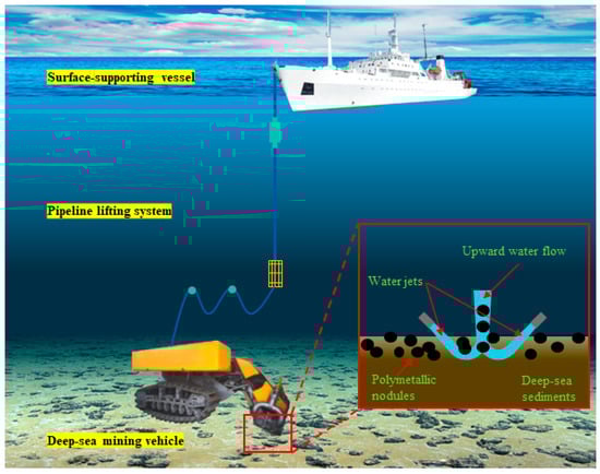
Figure 1.
Overview of the deep-sea hydraulic collection system.
To address these engineering challenges and research gaps, this study investigated the erosion mechanisms of submerged water jets on simulated sediments, aiming to provide more realistic experimental data and simulation references for the numerical modeling and equipment design of hydraulic nodule collection. To achieve this objective, a corresponding numerical simulation model has been developed, with key parameters calibrated based on the physical properties of the simulated sediments obtained from the validation experiments described in Section 3.
In reality, the physical properties of deep-sea sediments—such as density, viscosity, and moisture content—exhibit continuous variation with depth. However, in CFD simulations, accurately capturing this gradual transition requires an extremely fine mesh resolution and complex constitutive modeling, which can significantly increase computational costs and potentially lead to convergence difficulties. To address this challenge, we employed a stratified simplification approach, in which the sediment domain was divided into two layers based on depth-dependent volume-averaged physical properties, thereby approximating the vertical property variation. This method effectively reduces computational complexity. To determine the stratification depth, multiple samples were prepared during the experiment. Once the samples reached the saturated moisture content (109%), they were covered with water and allowed to stand for 24 h. After 24 h of settling, multiple measurements were conducted at different depths until the density of the lower layer closely matched the density corresponding to the saturated moisture content. This depth was defined as the stratification interface. The average moisture content of the upper layer was recorded as the reference value for simulation (note that any visibly separated water was removed during measurement). For clarity and consistency in the next sections, the upper sediment layer will be referred to as Su and the lower layer as Sl.
This study employed the EMF method to construct a simulation model in which water was treated as a liquid phase and the sediment particle flow was treated as a “continuous medium”. This approach eliminates the need to track individual particle movements; instead, it focuses on solving the volume fraction field and average velocity field of the entire particle phase. To characterize the flow behavior of this “continuous medium”, an “equivalent viscosity” (hereinafter referred to as viscosity) is introduced to represent the macroscopic flow resistance exhibited by the particle assembly during the flow process.
The simulation model is entirely established based on experimental data, including the tank dimensions, the placement of sediments with varying moisture content, and the defined boundary conditions (see Figure 2). The upper end of the water jet generation pipe is designated as the velocity inlet, where the specified velocity magnitude corresponds to the flow meter readings obtained during the experiment. The lower end of the pipe is connected to the entire fluid domain. The upper portion of the fluid domain outside the defined region is set as a pressure outlet with a gauge pressure of 0 Pa. All remaining boundaries within the fluid domain are configured as no-slip walls. During the initialization phase, the spatial position of the solid phase is defined using the region-marking method, and the corresponding regions are assigned solid volume fraction attributes through the region patch method. This volume fraction is calculated based on the experimentally measured moisture content of different sediment layers. Additional parameters, such as sediment particle size, density, viscosity, and moisture content, are detailed in Table 1.
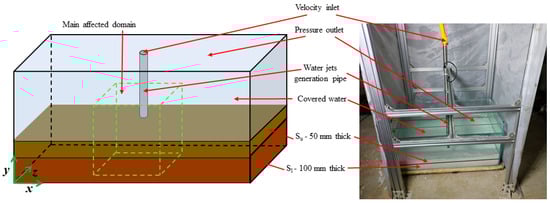
Figure 2.
Boundary condition setup of the simulation model and comparison with the setting of the experimental device.

Table 1.
Characteristic parameters of simulated sediments.
The entire computational domain is discretized using an unstructured tetrahedral mesh, with local grid refinement applied to the primary affected region, the water pipe, and the phase interface to accurately resolve flow behavior and interphase interactions. To eliminate the influence of spatial resolution on simulation accuracy, a mesh independence test was conducted, and convergence verification was performed for models with four distinct mesh densities. The volume fraction of Su at the third second within the monitoring plane—located 10 mm above the sediment surface in the main affected domain and covering a 100 × 100 mm area—is selected as the evaluation parameter (h = 40 mm, vf = 3 m/s).
As shown in Table 2, increasing grid density results in a significant improvement in computational accuracy. A comparative analysis of the results across the four grid configurations demonstrates that the error between Grid 4 and Grid 3 is negligible, indicating that further grid refinement would not lead to meaningful gains in accuracy. Therefore, considering the balance between computational accuracy and computational efficiency, Grid 3 is adopted as the optimal mesh configuration for this study.
Table 2.
Volume fraction of Su under four grid schemes.
3. Experiment and Simulation Validation
3.1. Simulated Sediment Preparation
The simulated deep-sea sediments must be prepared prior to the experiments, and its mechanical properties should be analyzed. Based on existing research, commonly used simulation materials include bentonite, kaolinite [14], diatomite [37], and quartz sand [25]. Among these, a mixture of bentonite and kaolinite with water produces simulated sediments that most closely resemble actual deep-sea sediments in terms of mechanical properties [14]. Currently, due to the different locations selected by researchers for deep-sea sediment studies, the resulting data vary. There is no standardized mixing ratio for simulating sediments. Therefore, different soil mixtures were validated based on in situ vane shear test data of deep-sea sediments (see Figure 3).
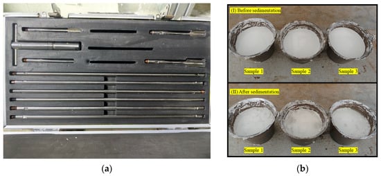
Figure 3.
Shear stress tests of simulated sediments following water coverage and sedimentation: (a) vane shear apparatus; (b) testing sample groups (Group I comprises three freshly prepared samples; Group II contains three samples that have been covered with water and sedimentation for 24 h).
The results indicate that when the mass ratio of bentonite to kaolinite is 2:1, the shear characteristics of the simulated sediments closely match the in situ data (see Figure 4). Three characteristic values were extracted from the shear curve, namely the maximum shear stress, the rotation angle at maximum shear stress, and residual stress. All of these values exhibit minimal deviation from the sea trial data, demonstrating that the samples accurately represent the mechanical behavior of actual deep-sea sediments.
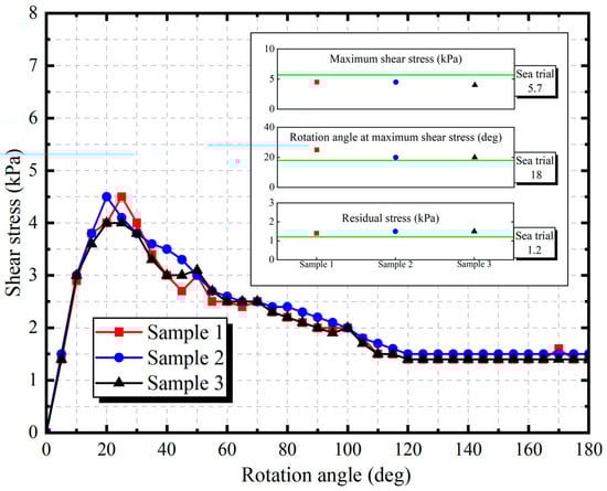
Figure 4.
Results of vane shear tests (the shear stress variation curves of three simulated sediment samples with the rotation angle of the shear plate are presented and compared with the in situ test results obtained at sea).
Additionally, in fluid mechanics studies, viscosity is a critical parameter for characterizing a fluid’s resistance to flow. Therefore, viscosity tests were conducted to measure the viscosity of sediments with varying moisture content. This not only further validates the accuracy of the simulated sediments but also provides fundamental data for subsequent simulations.
Viscosity tests were conducted on the two samples with different moisture content obtained in Section 2.2 (see Figure 5), and the resulting viscosities of the simulated sediments are presented in Table 1. Based on the viscosity data of deep-sea sediments reported by He et al. [38], it can be concluded that the viscosities of the simulated sediments prepared in this study fall within a reasonable range, thereby providing data support for numerical simulations.
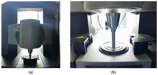
Figure 5.
Viscosity tests of simulated sediments: (a) rheometer for simulated sediment viscosity tests; (b) the viscosity test process of simulated sediments.
3.2. Experimental Platform Setup and Experimental Procedure
To further validate the accuracy of the EMF method in simulating deep-sea sediment behavior, an experimental platform for water jet impact on the simulated sediments was constructed (see Figure 6). The platform comprises a supporting frame, an experimental water tank, several water pipes, a 10 mm nozzle, a water pump, a flow valve, and a digital flow meter. The water jet velocity (vf) at the nozzle is precisely controlled through the coordinated use of the flow valve and digital flow meter, while the nozzle height (h) relative to the sediment surface is adjusted by moving the water pipe along the supporting frame.
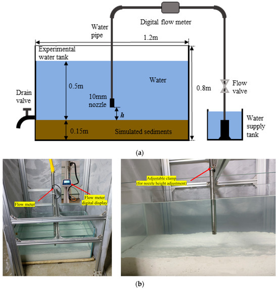
Figure 6.
Experimental platform: (a) schematic diagram; (b) experimental device.
Experimental Procedure:
- The flow valve was adjusted to achieve the designated flow velocity (vf).
- The water pipe was mounted on the supporting frame and set to the required nozzle height (h). During installation, the water pipe was completely filled with water to prevent air entrainment, which could otherwise compromise experimental accuracy.
- The water pump was activated to initiate the experimental run.
- Upon completion of each run, the turbid water in the tank was drained.
- Experimental data were collected, including measurements of erosion depth and the diameter of the erosion pit at the original sediment surface.
- The sediments were then restored to their initial conditions, the tank was refilled with water, and the system was allowed to stand for 24 h before conducting the next experiment.
3.3. Simulation Model Validation
In the validation of the simulation model, the focus was on evaluating the erosion depth (de) and diameter (di), as these two parameters provide an intuitive representation of the water jet’s impact on the sediments in both the vertical and lateral directions. The accuracy of the simulation model was further verified by comparing experimental data with simulation results, thereby enabling a comprehensive assessment of its predictive capability.
Figure 7 and Figure 8, respectively, present the simulation and experimental results under different water jet velocities (h = 20 mm; erosion time t = 10 s). Both sets of results exhibit the same trend in the evolution of erosion pit geometry (see Figure 9). However, as shown in Figure 9, the geometric dimensions of the erosion pits observed in the experiment are smaller than those obtained from the simulation. After analyzing the sedimentation characteristics, the authors suggest that this discrepancy may be attributed to further sedimentation occurring during the underwater stationary phase in the experiment. This additional sedimentation likely enhances the inter-particle forces among fine sediment particles, leading to the observed differences. However, due to current simulation limitations, the actual sedimentation process cannot be modeled, and this minor discrepancy must be neglected in the analysis. It is anticipated that future studies will address this limitation. When the water jet velocity increases from 1 m/s to 2 m/s, the erosion depth increases significantly. This may be because at lower velocities, the jet’s kinetic energy is insufficient to overcome the viscous forces of sediment particle flow. Once the jet velocity reaches 2 m/s, it can significantly overcome the viscous forces within the particle flow. Consequently, during the transition from 2 m/s to 6 m/s, the increase in erosion depth is no longer significant.
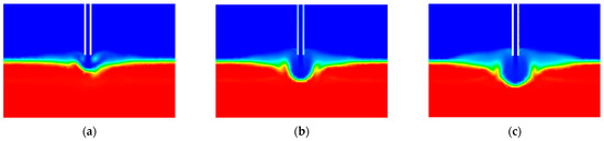
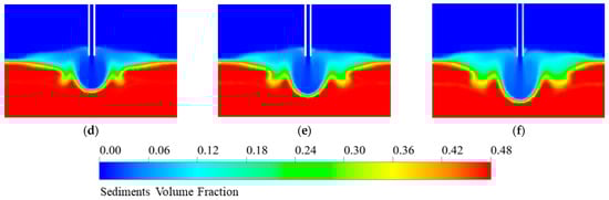
Figure 7.
Geometrical features of erosion pits in simulation: (a) vf = 1 m/s; (b) vf = 2 m/s; (c) vf = 3 m/s; (d) vf = 4 m/s; (e) vf = 5 m/s; (f) vf = 6 m/s.
Figure 8.
Geometrical features of erosion pits in experiment: (a) vf = 1 m/s; (b) vf = 2 m/s; (c) vf = 3 m/s; (d) vf = 4 m/s; (e) vf = 5 m/s; (f) vf = 6 m/s.
Figure 9.
Comparison of erosion pit geometries between simulation and experiment: erosion depth (de) and erosion diameter (di) (h = 20 mm, vf = 1–6 m/s).
Although secondary sedimentary phenomena cannot be explicitly simulated in numerical models, they result in corresponding changes in the mechanical properties of the sediments. However, through a systematic comparison of experimental and simulation results, it was further observed that the discrepancies were most significant when erosion was confined to the near-surface layer of the sediments. Nevertheless, as erosion depth increased, the deviation between the simulation and experimental results gradually diminished, and the final difference remained within 9%. This indicates that the consistency between the simulation model and the experimental data improves with increasing distance from the near-surface layer.
4. Results and Analysis
The erosion effects of different nozzle heights and water jet velocities were simulated using the validated numerical method. This section focuses on the analysis of the erosion processes and results, further elucidating the mechanisms of water jet interaction with the sediment.
4.1. Analysis of Two Different Erosion Mechanisms
An analysis of the simulation results reveals distinct erosion mechanisms under high and low water jet intensities, where jet intensity is determined by both nozzle height and jet velocity. Under high jet intensity, as illustrated in Figure 10a, the water jets rapidly lose kinetic energy during the diffusion process in water after exiting the nozzle. At a certain depth, the remaining kinetic energy is insufficient to overcome the greater resistance of the lower sediment layers, thereby limiting further erosion. At this stage, under the reaction force exerted by the sediments, a reverse flow develops (as shown by the velocity vectors in Figure 10b), which continues to affect the surrounding sediments (as shown in point A/A’ in Figure 11a and point C/C’ in Figure 11b). As depicted in Figure 12h, this reverse flow lacks the intensity to erode the lower sediment layers but exerts a more pronounced influence on the upper sediment layers, which exhibit lower erosion resistance. Consequently, this differential erosion leads to the formation of the erosion stratification zone observed in Figure 12h.
Figure 10.
The distribution diagram of water jet velocity and simulated sediment volume under high jet intensity (h = 40 mm, vf = 6 m/s, t = 0.90 s). (a) The contour of water jets velocity; (b) the contour of volume distribution of simulated sediments and vector map of water jet velocity.
Figure 11.
Different erosion mechanisms under different water jet intensities: (a) high water jet intensity; (b) low water jet intensity.
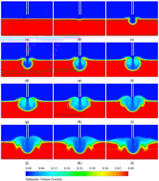
Figure 12.
Erosion process under high water jet intensity (h = 40 mm, vf = 6 m/s): (a) t = 0 s; (b) t = 0.04 s; (c) t = 0.14 s; (d) t = 0.30 s; (e) t = 0.60 s; (f) t = 0.90 s; (g) t = 1.40 s; (h) t = 1.80 s; (i) t = 3.00 s; (j) t = 5.00 s; (k) t = 7.00 s; (l) t = 10.00 s.
To be more specific, this reverse flow spreads laterally (points A/A’ in Figure 11a) and upward (points B/B’ in Figure 11a), continuing to interact with the surrounding sediments. The upward reverse flow eventually disperses the suspended sediments above, after which the sediments begin to settle. Subsequently, the erosion process gradually transitions into the stabilization phase. In contrast, the low-intensity water jets result in shallower erosion depths, and the reverse flow only affects the sediments near point C/C’ in Figure 11b without inducing uplift of the surface sediments. Therefore, only rapid downward erosion and limited erosion of the surrounding zones occur.
The erosion process under high jet intensity is detailed for the condition h = 40 mm, vf = 6 m/s. At t = 0 s, the sediments are in a static state. At t = 0.04 s, the water jets begin to contact the sediment surface and initiate the erosion process. The first stage of erosion lasts from 0.04 s to 0.14 s, after which the reverse flow starts to influence the surrounding and upper sediments, causing the surface sediment layer to arch upward. The lateral erosion rate increases, while the vertical erosion rate begins to decrease. At t = 1.8 s, due to the different mechanical properties of the upper and lower sediment layers, the jets’ erosive effect on the upper layer intensifies (see Figure 12h). The subsequent jets continue to act on the stratified zone, forming an erosion band around the erosion pit. After t = 3 s, the reverse flow breaks through the surface sediments and the sediment particles begin to settle, accumulating around the erosion pit, which visually reduces the erosion diameter. At t = 7 s, the erosion depth and diameter stabilize, with only minor changes observed thereafter. Subsequently, the sediment particles suspended in the water continue to settle, but their impact on both erosion depth and diameter remains minimal. Therefore, the numerical simulation is terminated at 10 s.
The erosion process under low jet intensity is detailed for the condition h = 100 mm, vf = 3 m/s (see Figure 13). At t = 0.3 s, the water jets contact the sediments and initiate the erosion process. The primary erosion in both the vertical and lateral directions continues until t = 3 s, at which point vertical erosion weakens, while the reverse flow enhances erosion of the surrounding sediment. This process lasts until t = 5 s, after which the shape of the erosion pit remains generally stable, with only minor changes observed.
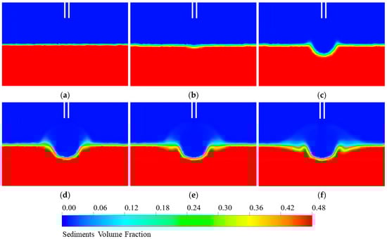
Figure 13.
Erosion process under low water jet intensity (h = 100 mm, vf = 3 m/s): (a) t = 0 s; (b) t = 0.30 s; (c) t = 0.80 s; (d) t = 3.00 s; (e) t = 5.00 s; (f) t = 10.00 s.
Upon analyzing the sediment response characteristics under high and low jet intensities, the erosion depth–time curves for sediments under these two conditions were investigated (see Figure 14). The results indicate that the erosion process in both scenarios can be categorized into three distinct phases, namely rapid erosion, steady erosion, and stabilization. The rapid erosion phase, lasting approximately 1 s, accounts for approximately 80% of the total erosion depth. Under high jet intensity, the steady erosion phase occurs between t = 1 s and t = 5 s. Subsequently, the slope of the erosion depth–time curve decreases, and the stabilization phase is reached at t = 7 s, where further increases in erosion depth become negligible. Under low jet intensity, the steady erosion phase also spans from t = 1 s to t = 5 s, during which the slope of the curve gradually diminishes. By t = 5 s, the stabilization phase is achieved, and the erosion depth remains virtually constant. Although the time required to reach stabilization differs between the two jet intensities, the overall trend remains consistent with the three-phase classification.
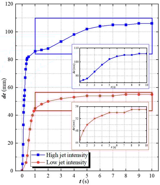
Figure 14.
Time-varying curves of erosion depth under high and low jet intensities.
4.2. Analysis of Erosion Results
After the erosion process concludes under each condition (as described in Section 4.1, with each erosion process lasting 10 s), the erosion depth and erosion diameter, serving as two key evaluation parameters, are statistically analyzed. This section focuses on investigating the influence of nozzle height and water jet velocity on these parameters.
As shown in Figure 15a, with the jet velocity held constant, the erosion depth decreases as the nozzle height increases. This trend is most significant within the range of h = 20–40 mm. When h > 40 mm, the rate of decrease in erosion depth markedly diminishes, and a linear variation is observed in the range h = 40–100 mm. As illustrated in Figure 15b, with the nozzle height held constant, the erosion depth shows a clear linear increase with increasing jet velocity (within the range studied in this paper).
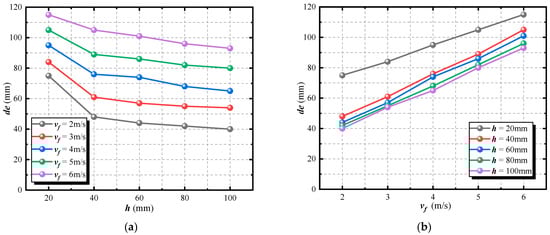
Figure 15.
Influence curve of erosion depth: (a) the curve of erosion depth varying with nozzle height at a constant jet velocity; (b) the curve of erosion depth varying with jet velocity at a constant nozzle height.
The effects of jet velocity and nozzle height on the erosion diameter were further analyzed. As shown in Figure 16a, at a constant jet velocity, the erosion diameter increases nonlinearly with increasing nozzle height, with the rate of increase gradually decreasing. This trend can be attributed to the significant diffusion of the water jet upon exiting the nozzle, which leads to a rapid expansion of the jet diameter. As the jet continues to interact with the surrounding water, the diffusion effect gradually diminishes. This phenomenon is consistent with the findings of Hu et al. [18] on the diffusion of submerged jets. In the range h = 20–40 mm, jet diffusion is rapid. However, when h > 40 mm, jet diffusion slows down, resulting in a slower rate of change in the erosion diameter. In the case of constant nozzle height (see Figure 16b), the erosion diameter also increases nonlinearly with increasing jet velocity, following a trend similar to that shown in Figure 16a. This behavior may be explained by the fact that at lower flow velocities (vf = 2–4 m/s), the reverse flow formed after the water jet impacts the sediment is relatively weak and has limited penetration into the upper sediment structure. Consequently, each increase in flow velocity significantly enhances the reverse flow, expanding its lateral spread and leading to a faster increase in the erosion diameter. However, as the jet velocity increases further (vf = 4–6 m/s), the reverse flow can easily break through the surface sediment, and the disturbance range begins to reach a saturation point. As the flow velocity continues to increase, the expansion of the reverse flow’s influence slows down, resulting in a reduced rate of increase in the erosion diameter.
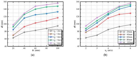
Figure 16.
Influence curve of erosion diameter: (a) the curve of erosion diameter varying with nozzle height at a constant jet velocity; (b) the curve of erosion diameter varying with jet velocity at a constant nozzle height.
5. Conclusions
This study presents a two-factor analysis of the erosion process of simulated deep-sea sediment under submerged water jet conditions, contributing to a better understanding of sediment–water jet interactions in deep-sea mining operations. The following key contributions were made:
- The mechanical characteristics of actual deep-sea sediments were used to prepare simulated sediments, which were then subjected to submerged water jet erosion experiments. Based on the experimental data, a numerical simulation model was developed using the EMF method to simulate sediment erosion under water jet conditions.
- The results indicate that two distinct erosion mechanisms can be identified based on jet intensity. Moreover, the erosion depth follows a clear time-dependent trend, which can be divided into three stages, namely rapid erosion, steady erosion, and stabilization. By comparing the erosion depth distribution characteristics at each stage, the dynamic evolution pattern of the erosion process is further elucidated.
- This study systematically analyzes the variation patterns of erosion depth and diameter under different combinations of jet velocity and nozzle height. The results reveal that erosion depth varies linearly with the independent variables (jet velocity and nozzle height), whereas the erosion diameter exhibits a nonlinear response.
Despite these findings, this study has certain limitations:
- The simulated sediments adopt a stratified structure, which cannot fully represent the continuous variation in mechanical properties typically observed in natural sediments.
- The simulation model does not account for secondary sedimentation during the settling phase, nor does it consider the enhanced inter-particle forces that may arise from this process. Consequently, this limitation may affect the accuracy of the conclusions.
- Although the simulation duration was designed to capture the main erosion stage and subsequent settling of suspended sediments, it does not fully consider the long-term diffusion processes that occur after erosion.
Future research will incorporate a more realistic sediment model to enable a more comprehensive analysis of the hydraulic response of sediments.
Author Contributions
Conceptualization, G.W. and C.L.; methodology, Y.Z. and G.W.; software, C.L. and Y.Z.; validation, Y.C. and B.C.; formal analysis, Y.C., B.C., and C.L.; investigation, G.W.; resources, Y.D.; data curation, C.L.; writing—original draft preparation, X.Z. and C.L.; writing—review and editing, G.W. and Y.Z.; visualization, X.Z.; supervision, X.Z. and Y.D.; project administration, Y.D.; funding acquisition, Y.D. All authors have read and agreed to the published version of the manuscript.
Funding
This study was supported by the science and technology innovation Program of Hunan Province [grant number 2024RC1001].
Institutional Review Board Statement
Not applicable.
Informed Consent Statement
Not applicable.
Data Availability Statement
The original contributions presented in the study are included in the article; further inquiries can be directed to the corresponding author.
Conflicts of Interest
Author Yangrui Cheng was employed by the company Changsha Research Institute of Mining and Metallurgy Co., Ltd. Author Bingzheng Chen was employed by the company Changsha Institute of Mining Research Co., Ltd. The remaining authors declare that the research was conducted in the absence of any commercial or financial relationships that could be construed as potential conflicts of interest.
References
- Balaram, V.; Armstrong-Altrin, J.S.; Khan, R.M.K.; Rao, B.S. Land and marine sedimentary deposits as potential sources of lithium. Int. Geol. Rev. 2025, 67, 1217–1250. [Google Scholar] [CrossRef]
- Du, K.; Xi, W.; Huang, S.; Zhou, J. Deep-sea Mineral Resource Mining: A Historical Review, Developmental Progress, and Insights. Min. Metall. Explor. 2024, 41, 173–192. [Google Scholar] [CrossRef]
- Guo, X.; Fan, N.; Liu, Y.; Liu, X.; Wang, Z.; Xie, X.; Jia, Y. Deep seabed mining: Frontiers in engineering geology and environment. Int. J. Coal Sci. Technol. 2023, 10, 23. [Google Scholar] [CrossRef]
- Miller, K.A.; Thompson, K.F.; Johnston, P.; Santillo, D. An Overview of Seabed Mining Including the Current State of Development, Environmental Impacts, and Knowledge Gaps. Front. Mar. Sci. 2018, 4, 418. [Google Scholar] [CrossRef]
- Jin, Y.Z.; Yao, Q.K.; Zhu, Z.C.; Zhang, X.M. Numerical Study and Parameter Optimization of a Dual-jet Based Large Particle Collection System for Deep-sea Mining. J. Appl. Fluid Mech. 2024, 17, 2215–2227. [Google Scholar]
- Gao, Y.; Xiang, X.; Li, Z.; Guo, X.; Han, P. An experimental and simulation study of the flow pattern characteristics of water jet impingements in boreholes. Energy Explor. Exploit. 2022, 40, 852–872. [Google Scholar] [CrossRef]
- Liu, B.; Wang, X.; Zhang, X.; Liu, J.; Rong, L.; Ma, Y. Research Status of Deep-Sea Polymetallic Nodule Collection Technology. J. Mar. Sci. Eng. 2024, 12, 744. [Google Scholar] [CrossRef]
- Yue, Z.Y.; Zhao, G.C.; Xiao, L.; Liu, M. Comparative Study on Collection Performance of Three Nodule Collection Methods in Seawater and Sediment-seawater Mixture. Appl. Ocean Res. 2021, 110, 102606. [Google Scholar] [CrossRef]
- Amudha, K.; Bhattacharya, S.K.; Sharma, R.; Gopkumar, K.; Kumar, D.; Ramadass, G. Influence of flow area zone and vertical lift motion of polymetallic nodules in hydraulic collecting. Ocean Eng. 2024, 294, 116745. [Google Scholar] [CrossRef]
- Su, X.H.; Chen, B.B.; Yang, H.; Ren, Y.; Wang, H.; Lin, R. Effects of nozzle angles of a double-row jet collector on harvesting performance. Ocean Eng. 2024, 301, 117573. [Google Scholar] [CrossRef]
- Dai, Y.; Zhang, Y.Y.; Cheng, Y.; Chen, J.; Zhu, X. CFD-DEM simulation and experimental investigations on continuous hydraulic sampling of deep-sea polymetallic nodules. Ocean Eng. 2024, 313, 119509. [Google Scholar] [CrossRef]
- Wang, P.J.; Li, L.; Wei, Q.-N.; Wu, J.-B. Study on Collection Performance of Hydraulic Polymetallic Nodule Collector Based on Solid-Liquid Two-Phase Flow Numerical Simulation. Appl. Sci. 2023, 13, 12729. [Google Scholar] [CrossRef]
- Becker, H.J.; Grupe, B.; Oebius, H.U.; Liu, F. The behaviour of deep-sea sediments under the impact of nodule mining processes. Deep Sea Res. Part II Top. Stud. Oceanogr. 2001, 48, 3609–3627. [Google Scholar]
- Liu, X.X.; Cheng, X.G.; Wei, J.; Jin, S.; Gao, X.; Sun, G.; Yan, J.; Lu, Q. Study on sediment erosion generated by a deep-sea polymetallic-nodule collector based on double-row jet. Ocean Eng. 2023, 285, 115220. [Google Scholar] [CrossRef]
- Chen, J.Q.; Zhang, G.H.; Si, J.-H.; Shi, H.; Wang, X. Experimental investigation of scour of sand beds by submerged circular vertical turbulent jets. Ocean Eng. 2022, 257, 111625. [Google Scholar] [CrossRef]
- Wang, C.; Wang, X.K.; Shi, W.; Lu, W.; Tan, S.K.; Zhou, L. Experimental investigation on impingement of a submerged circular water jet at varying impinging angles and Reynolds numbers. Exp. Therm. Fluid Sci. 2017, 89, 189–198. [Google Scholar] [CrossRef]
- Kartal, V.; Emiroglu, M.E. Effect of nozzle type on local scour in water jets: An experimental study. Ocean Eng. 2023, 277, 114323. [Google Scholar] [CrossRef]
- Hu, B.; Wang, H.; Liu, J.; Zhu, Y.; Wang, C.; Ge, J.; Zhang, Y. A Numerical Study of a Submerged Water Jet Impinging on a Stationary Wall. J. Mar. Sci. Eng. 2022, 10, 228. [Google Scholar] [CrossRef]
- Kartal, V.; Emiroglu, M. Local scour due to water jet from a nozzle with plates. Acta Geophys. 2021, 69, 95–112. [Google Scholar] [CrossRef]
- Bang, D.P.V.; Zapata, M.U.; Gauthier, G.; Gondret, P.; Zhang, W.; Nguyen, K.D. Two-Phase Flow Modeling for Bed Erosion by a Plane Jet Impingement. Water 2022, 14, 3290. [Google Scholar] [CrossRef]
- Mao, J.Y.; Si, J.H.; Chen, J.; Li, G.; Wang, X. Experimental investigation on sand bed scour by an oblique planar water jet at varying impinging angles. Ocean Eng. 2023, 279, 114526. [Google Scholar] [CrossRef]
- Hou, J.; Zhang, L.; Gong, Y.; Ning, D.; Zhang, Z. Theoretical and experimental study of scour depth by submerged water jet. Adv. Mech. Eng. 2016, 8, 1687814016682392. [Google Scholar] [CrossRef]
- Wang, H.L.; Jia, X.W.; Wang, C.; Hu, B.; Cao, W.; Li, S.; Wang, H. Study on the Sand-Scouring Characteristics of Pulsed Submerged Jets Based on Experiments and Numerical Methods. J. Mar. Sci. Eng. 2023, 12, 57. [Google Scholar] [CrossRef]
- Wang, C.; Jia, X.W.; Peng, Y.; Gao, Z.; Yu, H. Transient Sand Scour Dynamics Induced by Pulsed Submerged Water Jets: Simulation Analysis. J. Mar. Sci. Eng. 2024, 12, 2041. [Google Scholar] [CrossRef]
- Feng, C.; Kong, L.R.; Wang, Y.; Lu, J. Experimental study on scouring by submerged pulsed waterjet vertically impinging on cohesive bed. Ocean Eng. 2024, 298, 117308. [Google Scholar] [CrossRef]
- Taştan, K.; Koçak, P.P.; Yildirim, N. Effect of the bed-sediment layer on the scour caused by a jet. Arab. J. Sci. Eng. 2016, 41, 4029–4037. [Google Scholar] [CrossRef]
- Mohr, H.; Draper, S.; Cheng, L.; White, D. Predicting the rate of scour beneath subsea pipelines in marine sediments under steady flow conditions. Coast. Eng. 2016, 110, 111–126. [Google Scholar] [CrossRef]
- Mohr, H.; Stanier, S.A.; White, D.J.; Kuo, M. The variability of marine sediment erodibility with depth: Centimetric scale effects detected from portable erosion flume tests. Appl. Ocean Res. 2021, 113, 102721. [Google Scholar] [CrossRef]
- Dong, C.M.; Yu, G.L.; Zhang, H.; Zhang, M. Scouring by submerged steady water jet vertically impinging on a cohesive bed. Ocean Eng. 2020, 196, 106781. [Google Scholar] [CrossRef]
- Feng, C.; Kong, L.R.; Wang, Y.; Li, K.; Gao, Y. Numerical simulation of cohesive bed impinging by submerged pulsed and continuous waterjet based on SPH algorithm. Ocean Eng. 2024, 314, 119720. [Google Scholar] [CrossRef]
- Chen, C.; Pan, D.B.; Yang, L.; Zhang, H.; Li, B.; Jin, C.; Li, X.; Cheng, Y.; Zhong, X. Investigation into the Water Jet Erosion Efficiency of Hydrate-Bearing Sediments Based on the Arbitrary Lagrangian-Eulerian Method. Appl. Sci. 2019, 9, 182. [Google Scholar] [CrossRef]
- Zapata, M.U.; Bang, D.P.V.; Nguyen, K. Parallel simulations for a 2D x/z two-phase flow fluid-solid particle model. Comput. Fluids 2018, 173, 103–110. [Google Scholar] [CrossRef]
- Wang, B.Y.; Rhee, C.V.; Nobel, A.; Keetels, G. Modeling the hydraulic excavation of cohesive soil by a moving vertical jet. Ocean Eng. 2021, 227, 108796. [Google Scholar] [CrossRef]
- Qian, Z.D.; Hu, X.Q.; Huai, W.; Xue, W. Numerical simulation of sediment erosion by submerged jets using an Eulerian model. Sci. China Technol. Sci. 2010, 53, 3324–3330. [Google Scholar] [CrossRef]
- Yuan, Q.Q.; Zhao, M.; Wang, C.; Ge, T. Numerical study of sand scour with a modified Eulerian model based on incipient motion theory. Mar. Georesour. Geotechnol. 2018, 36, 818–826. [Google Scholar] [CrossRef]
- Tavouktsoglou, N.S.; Dimakopoulos, A.; Spearman, J.; Whitehouse, R.J.S. Application of Two Phase Eulerian CFD Model to Simulate High Velocity Jet Induced Scour. In Proceedings of the ASME 2020 39th International Conference on Ocean, Offshore and Arctic Engineering, Virtual Online, 3–7 August 2020; Volume 8. [Google Scholar]
- Wu, Z.Q.; Zhang, X.Z.; Jin, S.; Liu, J.; Liu, X.; Li, L.; Chen, F.; Chen, X.; Wei, J.; Li, H. Analysis of sediment disturbance and plume dispersion characteristics induced by deep-sea polymetallic nodule hydraulic collectors. Appl. Ocean Res. 2025, 156, 104462. [Google Scholar] [CrossRef]
- He, S.D.; Peng, Y.D.; Jin, Y.; Yan, J.; Wan, B. Simulated and Experimental Study of Seabed Sediments Sampling Parameters Based on the VOF Method. Chin. J. Mech. Eng. 2022, 35, 41. [Google Scholar] [CrossRef]


Disclaimer/Publisher’s Note: The statements, opinions and data contained in all publications are solely those of the individual author(s) and contributor(s) and not of MDPI and/or the editor(s). MDPI and/or the editor(s) disclaim responsibility for any injury to people or property resulting from any ideas, methods, instructions or products referred to in the content. |
© 2025 by the authors. Licensee MDPI, Basel, Switzerland. This article is an open access article distributed under the terms and conditions of the Creative Commons Attribution (CC BY) license (https://creativecommons.org/licenses/by/4.0/).