Abstract
A fundamental aspect in the evaluation of mining projects is the classification of mineral resources, as it directly influences the definition of mineral reserves and affects both the planning and operational phases of the mine. Traditional methods employed in the industry are based on geometric or geostatistical criteria which, while constituting the fundamental basis of the process, may prove insufficient when applied in isolation to reflect the uncertainty inherent in the databases used for the evaluation of mineral deposits. As discussed throughout the article, this limitation can lead to an incorrect or imprecise assignment of resource categories. This work presents a methodology to integrate variables related to sample quality as an additional criterion in resource classification. This allows for the identification of areas with greater uncertainty and the adjustment of their categories more consistently with data reliability. The effectiveness of the proposed method is demonstrated through its application to a real case study, complemented by a comprehensive analysis of its implications and results.
1. Introduction
The modeling and economic evaluation of a mineral deposit is primarily based on data obtained from drilling. These data are characterized by being point-based, limited in quantity, and potentially subject to errors. In other words, the data are subject to some type and degree of uncertainty [1,2,3]. Consequently, geological models are predominantly founded on subjective interpretations and interpolation/extrapolation techniques of the obtained data, rendering them inherently subject to a certain degree of uncertainty.
Geological uncertainty in the economic evaluation of mineral deposits is attributable to several factors: (i) style of mineralization (e.g., a deposit consisting of small veins or seams will have a higher degree of uncertainty than a massive deposit); (ii) the inherent variability in the material sampled; (iii) the representativeness of the sample; (iv) errors in the data itself (sampling, preparation, chemical analysis, and general processing of the data) [4]; (v) interpolation of grade, density; and (vi) calculation of recovery and dilution. While it is imperative to minimize all these sources of uncertainty, for example through the development of new Quality Assurance and Quality Control (QA/QC) methodologies [5], it is recognized that complete elimination of uncertainty remains unattainable. As a mining project progresses, uncertainty tends to decrease as more data are obtained and knowledge of the deposit increases.
In economic activities related to geology, uncertainty can lead to significant financial risks or inappropriate strategies, such as an incorrect definition of the life of mine plan (LoMP) or the necessary investments [6,7,8]. Therefore, it is not enough to build the best geological model; it is also imperative to locate and quantify uncertainties, thus identifying areas that may require further investigation. It is at this point that the classification of resources and reserves becomes pertinent. The classification of resources and reserves entails the categorization of the block model according to the degree of confidence in the estimates made (tonnes, grades, density, etc.). Therefore:
- A comprehensive evaluation of the project’s confidence is provided to relevant stakeholders, including mining partners, shareholders, and financial institutions involved in the project’s investment. This evaluation serves two primary purposes—first, to communicate the associated investment risk and, second, to prevent instances of fraud;
- The volume of the deposit has been determined for which sufficient information is available to support its inclusion in the calculation of an economic open-pit mine or in the design of an underground mine.
As will be detailed later, various methodologies, international systems, or codes have been developed to establish more or less standardized guidelines for the preparation of mining project evaluation reports. However, the methodologies for the classification of resources and reserves are defined only in a general manner and rely heavily on the subjective judgment of the qualified or competent person responsible for such classification. It is important to highlight that, in recent years, several mining projects have come under scrutiny due to significant flaws in their resource and reserve reports. Three representative examples that illustrate the potential failures are:
- The Telfer Au-Cu deposit, located in Western Australia, is characterized by mineralization occurring in multiple veins hosted within metasedimentary rocks that have experienced significant deformation due to folding and faulting [9]. In 2003, the company Newcrest Mining published the project’s feasibility study, which estimated a resource of 26.2 million ounces of gold (Moz Au), 0.96 million tonnes of copper (Mt Cu), and a reserve of 18.4 Moz Au and 0.69 Mt Cu [10]. Mining operations commenced in 2005 [11]. In 2006, the company updated these figures, reporting a resource of 24.6 Moz Au and 0.83 Mt Cu, along with a reserve of 17 Moz Au and 0.59 Mt Cu [11]. In 2007, another update reported a resource of 19.7 Moz Au and 0.73 Mt Cu [12], amounting to a 4.9 Moz Au reduction, equivalent to an 21% decrease from the 2006 report. The main reason for this reduction was the removal of positive adjustment factors that had been applied to the gold grade during resource estimation based on historical data and actual underground production [13]. These factors had been introduced due to the low gold recoveries obtained during drilling, caused by physical loss of gold in the sampling process. For the resource estimates, NQ diamond drill cores (48 mm diameter) were used [13]. Although the samples were of significant volume, they were still too small to define gold grades realistically [13]. The Telfer case demonstrates the “nugget effect” (heterogeneous Au distribution) in grade estimation, and the inherent difficulties in properly accounting for this phenomenon;
- The Boseto deposit (Botswana) consists of stratiform copper deposits hosted in sedimentary rocks [14]. In 2012, Discovery Metals Limited reported a mineral resource of 111.5 Mt at 1.4% Cu and 17.6 g/t Ag, and reserves of 21.8 Mt at 1.4% Cu and 18.2 g/t Ag [15]. However, when operations began, the forecasts were not met. The upper oxide layer, initially modeled at 30 m from the surface, was actually located at more than 60 m. This error was due to the lack of shallow drilling, as exploration efforts were focused on deeper parts of the deposit with the aim of increasing project resources [15]. This occurred because the deposits of the Kalahari Copper Belt are characterized as stratabound and quasi-vertical, a deposit type considered to have low geological uncertainty [16].The result was a short-term shortage of sulfide ore, as well as an open-pit design that was unsuitable for the actual deposit conditions: a pit that was too narrow and elongated. This led to a loss of confidence in the project by shareholders, ultimately resulting in the cessation of operations in 2015 and the sale of the project to Cupric Canyon Capital [13];
- Gold at the F2 Deposit (Phoenix Gold Project), located in Ontario (Canada), occurs in structurally controlled quartz–carbonate veins [17]. In 2013, Rubicon Minerals Corporation published the preliminary economic assessment of the F2 deposit of the Phoenix gold project [18]. This report, using a cut-off grade of 4.0 g/t Au, presented an indicated resource of 4.120 Mt at 8.52 g/t Au and an inferred resource of 7.452 Mt at 9.26 g/t Au. The revised estimate in 2016 (using a cut-off grade of 4 g/t Au) reported an indicated resource of 0.492 Mt at 6.73 g/t Au and an inferred resource of 1.519 Mt at 6.28 g/t Au [19].This implies a reduction of the indicated resources by 88% and of the inferred resources by 80%. The main cause of this decline was an incorrect interpretation of the orientation of the structures hosting the high-grade veins [13]. The influence of structural orientation on resource estimation was only recognized after trial underground mining had accessed the mineralized zones (operations began in 2014). A new report in 2018, using a cut-off grade of 3 g/t Au, established a measured resource of 0.188 Mt at 6.8 g/t Au, an indicated resource of 1.186 Mt at 6.3 g/t Au, and an inferred resource of 3.884 Mt at 6.0 g/t Au [20]. The resource figures were updated in 2020. Using a cut-off grade of 3 g/t Au, the estimate reported a measured resource of 0.391 Mt at 6.5 g/t Au, an indicated resource of 1.115 Mt at 7.49 g/t Au, and an inferred resource of 1.303 Mt at 6.5 g/t Au [21].
In recent years, numerous studies have been carried out on the evaluation of uncertainty and the classification of mineral resources. However, most of these works have focused mainly on the comparison and review of different methods [22,23], or on the development of novel approaches, such as resource classification using fractal models [24,25,26] or the application of machine-learning (ML) techniques [27,28]. Although these methods represent a valuable contribution to theoretical and methodological development, they have not yet achieved significant implementation in the mining industry.
Consequently, it is necessary to strengthen and improve the methods most commonly employed by the industry for mineral resource classification. In this context, the present article examines variables related to sample quality, which are often only superficially addressed in the classification process, and proposes a methodology to integrate them as an additional criterion. This approach makes it possible to identify areas of greater uncertainty and to adjust their categories more consistently with data reliability. Finally, the last section presents a real case study that assesses the impact of these factors on the outcomes of resource classification.
2. Material and Methods: Mineral Resource Classification
Resource classification is not necessarily a technical matter, but rather a self-regulated response by the mining industry to communicate investment risk, as well as a reaction to several notorious fraud cases. One of the most emblematic was the 1997 scandal involving the Busang gold prospect in East Kalimantan, Indonesia, led by Bre-X Minerals Ltd., Calgary, AB, Canada, which prompted the implementation of formal resource classification systems [29,30].
In recent decades, several international classification systems have been developed [31,32]. Among the most prominent are the Australian JORC Code [33], the Canadian National Instrument 43-101 (NI 43-101) [34], the South African SAMREC Code [35], the SME Guide for Reporting Exploration Results, Mineral Resources, and Mineral Reserves from the United States [36], the European Reporting of Exploration Results [37], and the classification system of the United States Geological Survey (USGS) [38]. Given the global nature of the mining industry, the Committee for Mineral Reserves International Reporting Standards (CRIRSCO) was established to create a set of standardized international definitions for reporting mineral resources and mineral reserves. These definitions and standards are known as the CRIRSCO International Reporting Template [39]. The main reporting codes are members of CRIRSCO and follow its core guidelines (Table 1). The JORC Code is the most widely accepted and is used as the standard in countries that do not have their own national code.
Out of these codes, all are similar, with minor differences in their definitions. Although they include accompanying guidelines, they are not systematic or formal in all technical aspects. The reporting codes use vague language in their definitions, as it is difficult to provide a general guideline applicable to all types of mineral deposits and resource estimation practices. All guidelines refer to geological continuity and grade as key components of the classification criteria. For example, the JORC Code provides the following definitions [33]:
- A ‘mineral resource’ is a concentration or occurrence of solid material of economic interest in or on the Earth’s crust in such form, grade (or quality), and quantity that there are reasonable prospects for eventual economic extraction. The location, quantity, grade (or quality), continuity and other geological characteristics of a mineral resource are known, estimated or interpreted from specific geological evidence and knowledge, including sampling. mineral resources are subdivided, in order of increasing geological confidence, into inferred, indicated, and measured categories;
- An ‘ore reserve’ is the economically mineable part of a measured and/or indicated mineral resource. It includes diluting materials and allowances for losses, which may occur when the material is mined or extracted and is defined by studies at Pre-Feasibility or Feasibility level as appropriate that include application of Modifying Factors. Such studies demonstrate that, at the time of reporting, extraction could reasonably be justified.
In other words, these are minimum standards or guidelines for practice, and are not intended to be used as enforcement tools. Therefore, the responsibility for ensuring appropriate disclosure lies with the technical competence of the individual or individuals who approve the resource calculations and classification, defined as the competent person (CP) or qualified person (QP). As a result, mineral resource classification is subjective and largely depends on the experience of the qualified or competent person [40,41]. A common misconception is that resource classification methods provide an objective assessment of confidence; indeed, the classification is a manifestation of the opinion held by the CP/QP.

Table 1.
CRIRSCO members and their reporting Standards.
2.1. Mineral Resource Classification Methodologies
Resource classification is carried out using a three-dimensional block model, where each block is assigned a category based on criteria that reflect the level of confidence in the estimation of grade, tonnage, and inferred density. The methodologies currently used for this purpose can be broadly grouped into three main approaches: (i) geometric methods, which evaluate the spatial distribution and quantity of available data using parameters such as the number of drill holes, the minimum number of samples per estimate, distance to the nearest drill hole, and average distance between drill holes [51,52,53]; (ii) variogram-based methods, which incorporate the spatial continuity of geology and/or mineral grades into the classification process [25,54,55,56,57]; and (iii) geostatistical simulation methods, which account for local variability in the data and aim to better quantify uncertainty when defining resource categories [23,24,26,41,58,59,60,61]. Geometric methods are used by industry in a broadly predominant manner compared to other approaches [23].
As demonstrated by several studies, e.g., [23,40,62,63], there is no coherence or consensus in the definitions of the parameters, and the qualified/competent person has (too) strong an influence on the process, as they frequently make different assumptions and decisions, often including arbitrary decisions in this process.
2.1.1. Geometrical Methods
Geometric methods for mineral resource classification rely on the proximity, quantity, and spatial distribution of the data (whether composites or the drill holes themselves) used in block model estimation. The most basic approach considers only the distance between the data and the estimated block, such as the distance to the nearest drill hole (or composite) or the average spacing between drill holes. This methodology is particularly applied when the drilling grid is regular [23]. However, this approach becomes overly simplistic when applied to irregular drilling grids, as it may produce artifacts. One such artifact involves assigning a high level of confidence to a block estimated from a single, very close data point, while interpolated blocks based on multiple samples may be assigned a lower confidence level due to a greater average distance (Figure 1). To mitigate such issues, the approach is often combined with an assessment of the number of available data points. This is typically achieved by defining a series of search ellipsoids, arranged from most to least restrictive. The determination of these ellipsoids can be made based on variogram ranges, for example at thresholds of 95%, 90%, and 80%, amongst others.
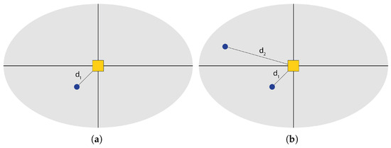
Figure 1.
(a) The block grade is interpolated from a single sample at distance . (b) The block grade is interpolated using two samples at distances and . Although b contains more information and thus higher confidence, if resource classification relies solely on sample distance, a would be assigned greater confidence since is smaller than the average distance in b.
The traditional geometric methods described above do not take into account the spatial distribution of data around the block being evaluated. If a block within the estimation area is surrounded by composites in all directions, it will present greater certainty than if there is a sector with no available information (Figure 2). To consider the spatial distribution of data within the search ellipsoid, the ellipsoid can be divided into halves, quadrants, or octants, with a minimum number of composites (or drill holes) required in each defined sector.
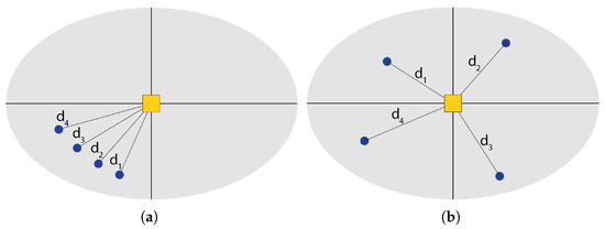
Figure 2.
(a) The block grade is interpolated from four samples located within the same sector of the ellipsoid. (b) The block grade is interpolated from four samples distributed across different sectors. If only sample distance and sample count are considered, both blocks would receive the same resource classification. However, b contains more spatially information and should therefore be assigned higher confidence.
2.1.2. Geostatistical Methods
Geostatistical methods use kriging variance for block model categorization. Blocks estimated with high kriging variance are considered less reliable than those with lower kriging variance [54,64,65,66]. This methodology accounts not only for the quantity and configuration of neighboring data but also for the spatial continuity of data through the variogram. The kriging variance, calculated for each estimated block, is essentially independent of the actual data values used in the estimation and depends solely on the spatial configuration of the local data employed in the estimation process. The link between the variance and the data values exists only through the variogram, which is global rather than local in its definition [67,68,69,70]. In practice, this criterion requires defining a variance threshold between categories [66,71,72,73]. The kriging variance thresholds used for classification are determined according to the mineralization style, the QP’s expertise, or the drilling grid employed, e.g., the kriging variance of a block located at the center of a drillhole grid can be used as the upper threshold for resource classification [74].
One of the advantages of using kriging variance as a classification criterion is that it incorporates the spatial structure of the variable and the redundancy between samples. However, this approach can lead to classification maps with undesirable artifacts, particularly in the vicinity of sampled points, where kriging variance tends to be very low. It is also important to note that kriging (and therefore kriging variance) is calculated under the assumption of homoscedasticity, meaning that the error variance in estimating the grade of a block is independent of the actual magnitude of the variable. However, grades in mineral deposits typically exhibit heteroscedasticity: data variability increases with higher values (also known as the proportional effect). This can result in an underestimation of uncertainty in high-grade regions and an overestimation in low-grade areas. Consequently, the resulting resource classification may be unrepresentative.
It is important to note that kriging variance refers to relative thresholds, as it does not have a direct physical or geological meaning. Therefore, the definition of thresholds for each category largely depends on subjective criteria. In this regard, the method can be considered analogous to the drillhole spacing approach, but implemented within a formal geostatistical framework.
Since it relies on statistical methods, it is essential that the data population is sufficiently large, that is, that an adequate number of samples is available to support a reliable geostatistical analysis. When this is the case, and the variation in values with distance can be modeled using one of the typically employed curves (lognormal, spherical, Gaussian, etc.), Kriging can be considered the most suitable method for advanced exploration projects. However, it is not as appropriate for early-stage projects, where data are still limited.
2.1.3. Conditional Simulation
Conditional simulation is a geostatistical tool that allows for the generation of multiple equally probable realizations of a regionalized variable. These realizations are conditioned on the existing sample data and the spatial structure defined by the variogram model [3,58,73,75]. Unlike deterministic methods such as kriging, which provide a single smoothed estimate, conditional simulation preserves the true variance in the data. The uncertainty for each block in the model is quantified based on the set of generated realizations (for each estimated block, a distribution of simulated values is obtained that satisfies the imposed conditions). From this distribution, it is possible to calculate confidence intervals, which describe the probabilistic behavior of the variable at that location. In an area with a high sampling density, the variability among the multiple simulations of the variable is expected to be lower than in a part of the deposit with sparse sampling. However, even in densely sampled areas, when the local grade variability is high, elevated values of the coefficient of variation can still be expected.
In general, the mining industry has been reluctant to adopt conditional simulation, as processing multiple realizations for large mineral deposits is both time-consuming and complex [3]; however, its use is becoming increasingly common [73]. Some authors, e.g., [51], recommend its use only as a supporting tool, arguing that final classification should remain based on geometrical criteria. This stems from the fact that results are highly sensitive to the modeler’s assumptions and input parameters, potentially reducing transparency for investors.
2.2. Modifying Factors in Resource and Reserve Estimation
As mentioned in the previous section, the methods commonly used in the industry to classify mineral resources focus primarily on geometrical factors or the spatial continuity of the data. However, these approaches often overlook other critical aspects, such as data quality, reliability, and sample size. Relying on a single quantitative criterion for mineral resource classification is rarely appropriate and frequently results in suboptimal outcomes. Integrating multiple criteria, both quantitative and qualitative, is a complex process that requires careful analysis to avoid inconsistencies. Four key aspects are rarely addressed in mineral resource classification: (i) drilling type, (ii) core recovery, (iii) sample size, and (iv) historical data. The following section analyses the relevance of these factors and their integration into the process of mineral resource classification, with the aim of establishing a methodological framework designed to reduce the uncertainty inherent in such processes. The proposed approach enables the transparent identification and representation of the main sources of uncertainty, while defining a clear, replicable, and traceable workflow that can be followed by other professionals or researchers in the field.
2.2.1. Drilling Techniques
Drilling aims to assess the mineral grades of known deposits as well as to study the geology of potential sites. Depending on the purpose and budget of the project, there are various drilling methods available. The most commonly used techniques are reverse circulation (RC) drilling and diamond drill hole (DDH) drilling.
DDH drilling is the most widely used method for mineral deposit exploration. It is a more expensive and slower form of drilling, and it requires a constant and significant supply of water. However, unlike RC drilling, it is capable of retrieving an unaltered cylindrical core of rock, preserving the structural details of the underlying geology. In addition, it allows for the generation of oriented drill holes. DDH drilling allows for the generation of oriented cores. Oriented core is required in a variety prospect types and mineral deposits. It is critical to assessing 3D geometry in prospects containing moderate to strong folding, or arrays of variably oriented faults or shear zones, or of variably oriented mineralized vein systems. It is very important in the analysis of fracture patterns for geotechnical assessment and it is very useful in the statistical analysis of vein patterns. An example of this is mineralization associated with structural controls, such as Sn-(Ta-Li) and W-(Sn) deposits (Figure 3), or quartz-carbonate-Au veins, like those previously observed in the F2 deposit (Phoenix Gold Project), where an incorrect interpretation of the orientation of the structures hosting high-grade veins led to an overestimation of the deposit’s resources.
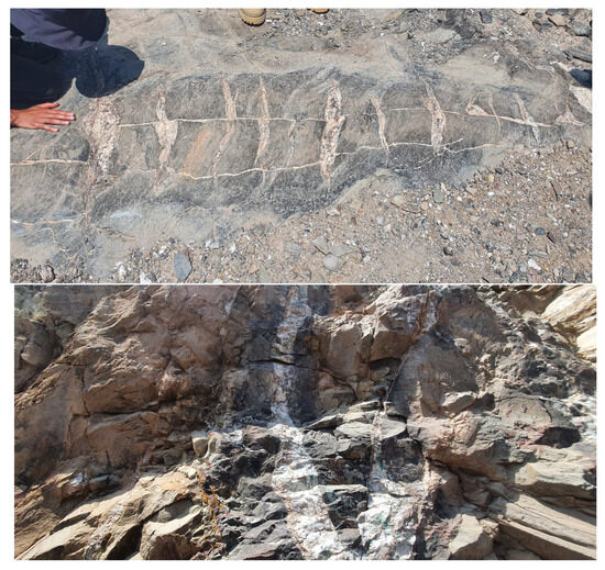
Figure 3.
Sheeted and anastomosing system of quartz–sulphide–cassiterite–wolframite veins hosted in metasedimentary rocks at the Brandberg West mine (Namibia). Photograph taken in September 2024.
Reverse circulation6 (RC) drilling is a technique that enables the collection of small rock chip samples ranging in size from a few centimeters to a few millimeters. It is relatively inexpensive and does not require water. Moreover, under certain ground conditions, RC may be the only viable method, as it is relatively insensitive to challenging soil conditions (such as fractured rock, permafrost, glacial till, etc.) that can be problematic for other drilling methods. However, this methodology presents two major drawbacks when compared to DDH drilling: (i) difficulty in core logging, along with imprecise estimation of depths and thicknesses, which hampers the accurate definition of mineralized domains; (ii) loss of structural information, which limits geological and geotechnical interpretation.
Grades obtained through RC drilling are generally associated with greater uncertainty compared to those derived from DDH. Although RC drilling is effective for delineating the extent of mineralized bodies and characterizing massive ore deposits, it is not considered the most appropriate method for resource evaluation, particularly in the early stages of exploration. A block may initially be classified with a high level of confidence due to the high sampling density provided by RC; however, the actual uncertainty may be significantly higher.This discrepancy may require a reduction in the confidence level and, consequently, lead to a reclassification of the resource.
2.2.2. Drill Core Recovery
The total or partial loss of core material during DDH drilling, and consequently the loss of information, is a common occurrence. The loss of drilling core recovery (Figure 4) gives rise to the following issues: (i) difficulty in core logging, along with imprecise estimation of depths and thicknesses, which hampers the accurate definition of mineralized domains; (ii) loss of structural information, which limits geological and geotechnical interpretation; (iii) biased sampling, both due to the lack of material and the difficulty in making an accurate longitudinal split of the core; (iv) difficulty in accurately estimating the grade. If the lost material has a lower grade than the recovered section, the result is an overestimation of the grade, potentially leading to the inclusion of a sample in the ore zone that should, in fact, have been classified as waste. Conversely, if the lost material has a higher grade, an underestimation occurs; (v) difficulty in accurately determining the density of the sample, and thus in calculating a reliable tonnage.
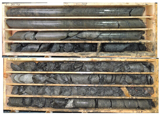
Figure 4.
Core interval with poor recovery at the transition between massive sulphide and underlying stockwork mineralisation.
Despite the aforementioned problems, under-recovery is rarely reported in detail in resource and reserve classification reports. In codes that adhere to the CRIRSCO guidelines (Table 1), drill core recovery is only mentioned in passing, e.g., the JORC Code, 2012 Edition [39], states the following: “Additional disclosure is particularly important where inadequate or uncertain data affect the reliability of, or confidence in, a statement of Exploration Results; for example, poor sample recovery…”. Likewise, the JORC Code emphasizes the importance of drill sample recovery to ensure their representativeness and to accurately record the value of core recovery obtained. This is aimed at assessing potential biases resulting from the loss of fine and/or coarse material. In other words, the CRIRSCO codes highlight the importance of disclosing such information; however, it is rarely reported, or when it is, the level of detail provided is often insufficient. Moreover, this topic is scarcely addressed in the literature. Some authors, e.g., [76], propose classifying drill samples according to recovery ranges and interpolating this information into each block of the model. However, they do not propose any methodology for integrating this information into the final classification of the block model. To integrate core recovery data with resource and reserve classification, the authors of this article propose the following methodology:
(i) Calculate a core recovery value for each composite. The most common ones are defined below.
Total Core Recovery (TCR) is defined as the percentage of the drill core that has been successfully recovered, whether obtained through diamond drilling (DDH) or reverse circulation (RC) drilling.
Solid Core Recovery (SCR) is the percentage of drill core recovered as intact sections whose length is equal to or greater than the drill hole diameter, relative to the total core advance length.
Rock Quality Designation (RQD) is the percentage of core recovery consisting of intact core pieces with a length of 10 cm or more, expressed as the ratio of the length of these pieces to the total length of the core run.
SCR and RQD are parameters used in geotechnics for rock mass classification as they are easy and quick to calculate. Among these, RQD is the most commonly used and is often the only method applied for rock mass classification, as it is a key component of the Rock Mass Rating (RMR) system [77,78,79] and the Norwegian Geotechnical Institute Q-system (“Q”) [80,81,82,83].
(ii) Interpolation of the previously defined parameters. In this way, a block model of rock mass quality is obtained.
(iii) Validation and analysis of the interpolated values.
(iv) Integration of drill core quality with the previously assigned resource classification. This integration can be carried out using acceptable ranges of some of the previously defined parameters for each resource category. Consequently, although a block may initially be classified with a high level of confidence, for example, as “measured” due to high sampling density, poor core recovery quality could justify its reclassification to a lower confidence level.
This reclassification can be implemented quickly and easily using SQL, For example, with the CASE statement (Algorithm 1). This instruction evaluates a series of conditions and returns a value when the first condition is met (similar to an if-then-else structure). Once a condition is satisfied, the evaluation stops and the corresponding result is returned. If none of the conditions are true, a value defined in the ELSE clause can be returned; otherwise, it returns NULL.
| Algorithm 1 SQL code for integrating recovery values into resource classification. The parameters threshold_high and threshold_low are user-defined values that should be adjusted according to the characteristics of each mineral deposit.SQL code for integrating recovery values into resource classification. |
SELECT CASE WHEN recovery >= threshold_high AND precision = ’Measured’ THEN ’Measured’ WHEN recovery >= threshold_low AND precision = ’Measured’ THEN ’Indicated’ WHEN recovery < threshold_low AND precision = ’Indicated’ THEN ’Inferred’ ELSE ’Inferred’ END AS classification FROM resource_table; |
2.2.3. Historical Data
When evaluating mineral deposits, it is common to have extensive databases of historical drilling data used in previous estimations. While this is clearly of great value, ensuring that the data and interpretations from these drillholes are robust is not always straightforward.
As a general rule, historical data should never be trusted implicitly, since it invariably reflects the standards and understanding of the time at which it was collected. Whenever an existing mineral resource is updated based on historical drilling data, both the data and previous interpretations must be thoroughly reviewed and verified. Historical data are often not collected in accordance with current industry best practices, such as accurate drill hole deviation measurements, precise collar positioning, assay quality, the number of elements analyzed, and QA/QC procedures. Consequently, historical datasets are unlikely to provide a comprehensive and reliable depiction of mineralization.
Even after thorough verification, they may still be of insufficient quality and, in many cases, are directly excluded from the database used for resource classification. However, the data can still provide valuable geological information to help understand the deposit, its extent, and potential morphology, thereby accelerating subsequent exploration and enabling significant cost savings. For this reason, historical drillholes with a high degree of uncertainty are not suitable on their own for resource classification, particularly for the higher resource categories.
Similar to what was shown for the previous modifying factors, each composite can be assigned a value based on its age and the associated level of confidence. In this way, each block will be assigned a confidence value. For the higher resource classifications, only blocks that meet a minimum confidence level will be considered.
2.3. Methodology for the Implementation of Modifying Factors
Numerous authors, e.g., [84,85], emphasize the need for a standardized workflow to develop robust geological models. Such a workflow enables efforts to be focused on well-defined tasks, ensures data consistency, and facilitates reproducible results by different users using the same input data and parameters. Figure 5 illustrates the proposed generalized workflow developed to incorporate the parameters analyzed in this section into the process of mineral resource reclassification. This framework provides a structured and systematic approach, facilitating the transparent integration of multiple criteria and enhancing the robustness, reproducibility, and traceability of the classification outcomes.
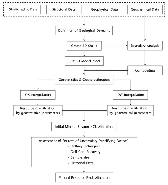
Figure 5.
Proposed generalized workflow for integrating the parameters analyzed throughout this section into the reclassification of mineral resources.
The key elements encompassed within the proposed flowchart are outlined below, highlighting the principal stages and decision points that underpin the methodology and guide its practical implementation:
- Data collection and validation: Data are collected, standardized, and integrated. A three-dimensional (3D) visualization is recommended to identify and correct errors such as incorrect coordinates, duplicate records, or georeferencing issues.
- Geological model construction: The geological model is constructed through the integration of lithological data and assay results. This enables the interpretation of the deposit geometry and the definition of distinct mineralized domains.
- Block model generation: Once the mineralized bodies have been defined, they are subdivided into blocks. The dimensions of each block depend on the morphology of the mineralized body, the spatial distribution of the data, and the planned mining method (e.g., bench height in open-pit mining).
- Grade interpolation: Grade estimation is carried out using methods such as Inverse Distance Weighting (IDW) or geostatistical techniques like Ordinary Kriging (OK). The selection of the interpolation method should consider the availability and spatial distribution of the data. Each mineralized domain must be interpolated independently, as different domains often require specific parameters.
- Initial resource classification: This stage is conducted using either geometrical or geostatistical methods. Each mineralized domain must be classified independently to assign the appropriate resource category.
- Application of modifying factors: Each modifying factor is assessed individually, and its effects are validated both numerically and visually, typically through sectional analysis.
- Mineral resource reclassification: All outputs from the previous stages are integrated to produce a comprehensive final classification of the mineral resources.
3. Results: Application to Case Study
This section presents an analysis of the impact of the various parameters described in Section 2.2 on resource classification in a real-case scenario. For the purposes of this study, the Tom West deposit was used as a reference. The 3D modeling, block model construction, and the different resource classifications were undertaken using RecMin software version 7.08. [86], while the geostatistical analysis was performed with RecMin Variograms version 1.0.0.30. [87,88]. Both software packages are freeware. It should be emphasized that this study is purely academic in nature and is not driven by economic objectives.
3.1. Geology Setting
The Tom deposit is located in Macmillan Pass, in the Yukon Territory (Canada), near the border with the Northwest Territories (NWT). The Tom deposit comprises several stratiform Zn-Pb-Ag-Ba orebodies (Tom East, Tom Southeast, and Tom West) of the sedimentary exhalative (SEDEX) type (Figure 6). The Tom deposit lies within a north–south-trending anticlinorium. Tom West is situated on the western limb of the fold, while Tom East is located on the eastern limb. Tom Southeast is positioned around the southern bend of the fold. It is interpreted that the Tom West and Tom East orebodies, both of which outcrop, originally formed a single orebody [89]. In contrast, the Tom Southeast orebody is interpreted to have formed in a sub-basin separate from the main graben structure that hosts the Tom West and Tom East zones [89].
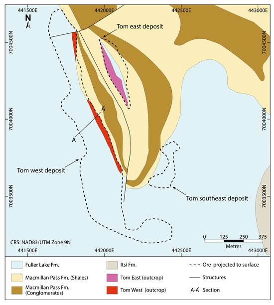
Figure 6.
Geological map of the Tom deposit. Section A–A’ is shown in Figure 7.
The mineralization ranges from well-laminated and stratiform (parallel to the sedimentary bedding) to a brecciated, stockwork-style zone adjacent to the Tom normal fault. At Tom, the mineralization has segregated into distinct facies along vertical and lateral transitions from darker to lighter colors of sphalerite, accompanied by a progressive decrease in Pb/Zn ratios. This indicates an increasing distance from the feeder zone [89,90]:
- Vent facies: Stockwork composed of pyrite, pyrrhotite, galena, and sphalerite, with minor amounts of chalcopyrite, arsenopyrite, and tetrahedrite, within a gangue of ferroan carbonates, quartz, and barite. This facies includes an upper high-grade zone, with Pb+Zn contents ranging from 15–30%, silver between 150 and 200 g/t, and a low Zn/(Zn+Pb) ratio.
- Pink facies: Interbedding of barite, chert, cream-colored sphalerite, fine-grained pyrite, and black barium carbonate, overprinted by pink and yellow sphalerite. This assemblage results in locally high grades, in the range of 10–30% Pb+Zn.
- Grey facies: Interlayered pink sphalerite, galena, and fine-grained pyrite, associated with white to pale grey barite, light grey chert, and grey to white barium carbonate or feldspar. Typically yields Pb+Zn grades in the range of 4–5%, with negligible silver content.
- Black facies: Black shale and chert interbedded with barite, witherite (barium carbonate), and fine-grained sphalerite, galena, and pyrite. Grades generally range from 4–10% Pb+Zn, with a high Zn/(Zn+Pb) ratio.
The Tom West mineralized body dips at 60° to the southwest, extending approximately 1 km along a north–south strike and reaching up to 400 m down-dip. Its maximum thickness is around 60 m. The previously described facies are well defined within the Tom West mineralized body (Figure 7).
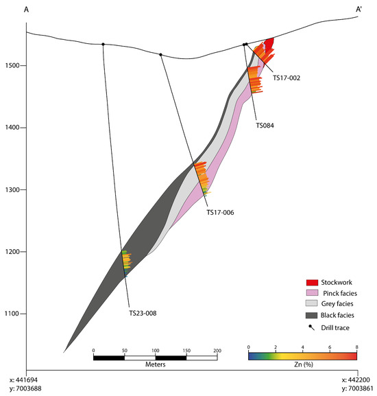
Figure 7.
Geological cross-section of the Tom West deposit.
3.2. Input Data
The data utilized in this study originate from the Tom West deposit and have been made publicly accessible by FIREWEED METALS CORP. [91]. A total of 2666 samples from 115 drillholes have been analyzed. The variables considered in this case study include: zinc grades (Zn), metallurgical recovery (classified as “Yes” for samples with recovery less than or equal to 85%, and “No” for those with recovery above 85%), drill core diameter, and the year each drillhole was conducted. The drillholes included in this study are grouped into three distinct phases:
- 97 historical drillholes drilled before 2011: conducted between 1952 and 1980 using diamond drilling (DDH) techniques. Various core diameters were used during this phase, including: EX (38.1 mm core size diameter), AX (48.5 mm core size diameter), AQ (27.0 mm core size diameter), BQ (36.5 mm core size diameter), NQ (47.6 mm core size diameter), and HQ (63.5 mm core size diameter);
- 11 drillholes drilled by Hudbay in 2011: all campaigns during this phase were conducted exclusively using HQ diameter core;
- 47 drillholes drilled by Fireweed since 2017: consisting of widely spaced drill holes, using HQ and NQ diameter cores.
3.3. Geological and Geostatistical Modeling
The three-dimensional model of the Tom West mineralized body was developed using RecMin software, based on the triangulation of 36 geological cross-sections (Figure 8). The mineralized horizon was delineated using samples containing ≥1 wt%. The resulting model defines a mineralized body with thicknesses ranging from 10 to 60 m, striking at 340° and dipping at 60°. The mineralization exhibits a well-defined contact with the hosted rock (Figure 9).
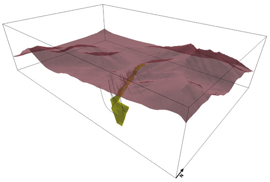
Figure 8.
3D model of the Tom West orebody.
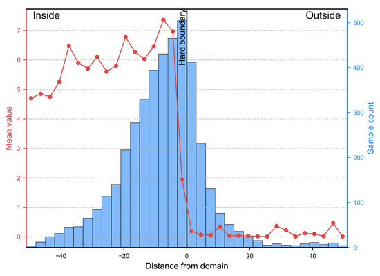
Figure 9.
Boundary plot of the Zn samples.
In order to generate composites of uniform length, an analysis of sample lengths was carried out. As shown in Figure 7, of the 2666 assays included within the modeled volume, 40.3% correspond to samples with a length of 1 m, while 30.6% are 1.5 m in length (Figure 10). To ensure consistency and to avoid subdividing assay intervals, a composite length of 1 m was selected, as it represents the most frequently used sampling interval in the Tom West dataset.
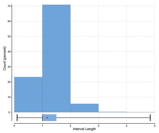
Figure 10.
Histogram and box plot of the lengths of the samples from Tom West.
The Tom West mineralized body contains a sufficient number of samples to support the construction of representative variogram models. Experimental variograms were calculated along the directions corresponding to the major, semi-major, and minor axes of anisotropy (Figure 11).
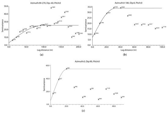
Figure 11.
Unidirectional experimental variograms: (a) Major Axis Variogram, (b) Semi-Major Axis Variogram, (c) Minor Axis Variogram.
The configuration employed consisted of 10 lag intervals with a lag separation distance (L) of 10 units, an angular tolerance (T) of 10 degrees, and a search tube radius (B) of 15 units, defining the spatial volume within which data pairs were considered. To ensure statistical robustness and representativeness, only variogram points with more than 300 data pairs were retained.
The three experimental variograms were modeled using a spherical variogram model. Finally, a block model was generated using blocks measuring 3 × 3 × 3 m, comprising a total of 696,874 blocks. Zinc grades were interpolated using the IDW method, with parameters derived from the variogram models (Table 2).
Table 2.
Axes and ranges of the search ellipsoid calculated from the variograms in Figure 11.
3.4. Mineral Resources Classification: Sensitivity Analyses
Four resource classifications were made using the categories defined by the NI 43-101 standards: (i) traditional resource classification, based on the number of composites and their distance to the estimated block; (ii) resource classification incorporating, in addition to the previous criterion, parameters related to drill core recovery; (iii) resource classification adding to the first case parameters related to the drilling method and its age; and (iv) resource classification integrating all the aforementioned parameters.
3.4.1. Case Study 1: Traditional Approach
An initial resource classification was carried out based on the number of composites and their distance. The distances to composites (Table 3) were defined according to the variograms calculated in the previous section. For the inferred resource category, the maximum variogram range was used as the limit; for indicated resources, half of this range; and for measured resources, one tenth of the distance. Additionally, for the measured and indicated resource categories, the presence of at least two drillholes located in opposite quadrants, with an angular separation greater than 90°, was required.
Table 3.
Resource classification parameters.
The parameters established in Table 3 allowed the zones closest to the surface of the deposit to be classified as indicated, and the middle zone as inferred (Table 4 and Figure 12). However, the deeper sections of the mineral body were not classified due to the lack of drill holes. The low drill hole density prevents the assignment of the measured resource category.
Table 4.
Results from the resource classification.
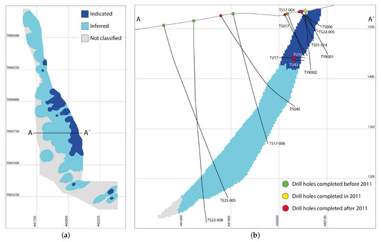
Figure 12.
Visual representation of the results obtained for resource classification in Case Study 1: (a) overhead view of Tom West’s block model; (b) cross-section of the central portion of Tom West’s block model.
3.4.2. Case Study 2: Recovery Analysis
In the original database, core recovery is marked as “No” for samples with a recovery greater than 85%, and “Yes” for those with a recovery equal to or less than 85%. Samples classified as “No” were assigned a recovery value of 100%, while those labeled “Yes” were assigned a recovery value of 85%. The core recovery data were interpolated using the same parameters applied to the interpolation of Zn grade.
To integrate the recovery values with the resource classification carried out in Case 1, a minimum recovery of ≥95% was established for the indicated category. As a result, blocks initially classified as indicated that do not meet this threshold will have their category downgraded to inferred.
As shown in Figure 13a, the blocks with a recovery <95% are generally distributed in small clusters, without displaying any well-defined spatial continuity. An exception to this pattern is a subtle alignment of blocks in the northern sector of the deposit, oriented NW–SE. This discontinuous distribution is generally attributed to the presence of minor faults or internal structures within the mineralization. The new resource classification (Table 5) reveals a 13% reduction in the number of blocks classified as “indicated” compared to the classification presented in Case Study 1.
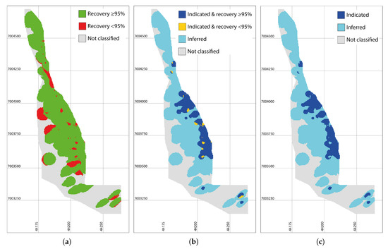
Figure 13.
Study of drilling core recovery in resource classification: (a) definition of blocks with recovery below 95% (red blocks); (b) integration of resource classification from Case Study 1 with blocks showing recovery below 95% (yellow blocks); (c) final resource classification result.
Table 5.
Resource classification results from Case Study 2 and their comparison with those from Case Study 1.
3.4.3. Case Study 3: Analysis of Drilling Techniques and Historical Data
As previously noted, the Tow West deposit database includes a large number of historical drill holes with varying diameters, most of which are relatively small. To account for this variability, a quality value of 0 was assigned to samples from drillholes completed prior to 2011, whereas samples from the 2011 and 2017 campaigns were assigned a quality value of 100. These parameters were interpolated using the same criteria applied in the Zn grade interpolation (Table 2). In this way, it is possible to determine whether the interpolated grade of each block is based on data from older or more recent drillholes.
As shown in Figure 14a, the areas drilled through boreholes conducted since 2011 exhibit a widely dispersed spatial distribution. This suggests that the majority of the resources classified as indicated in Case Study 1 originate from older drilling campaigns, thereby undermining their reliability. When applying a quality filter of ≥75 to the blocks classified as indicated in Case Study 1 (Figure 14a,b), a significant reclassification is observed: 73.3% of these blocks are reclassified as “inferred” (Table 6). This reclassification results in small, disconnected clusters of blocks that retain the indicated category (Figure 14c).
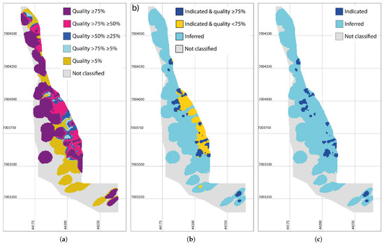
Figure 14.
Study of the type and reliability of drillings in resource classification: (a) definition of blocks according to quality level; (b) integration of resource classification from Case Study 1 with blocks of quality < 75% (yellow blocks); (c) final resource classification result.
Table 6.
Resource classification results from Case Study 3 and their comparison with those from Case Study 1.
It is important to highlight that the regulations aligned with CRIRSCO standards emphasize the necessity for resource classifications—particularly in the higher categories—to be supported by demonstrable geological continuity. This requires a comprehensive interpretation based on the spatial coherence of multiple drillholes, rather than relying on isolated observations from individual drillholes. In numerous resource classifications, concentric rings of measured and/or indicated resources can be observed around drillholes, separated by inferred and/or unclassified blocks. This pattern is known as the “Spotted Dog”. Although this pattern does not clearly form in Case Study 3, the reclassification shown in Figure 14c clearly illustrates a loss of geological continuity in the blocks classified as indicated. Therefore, further analysis and a more rigorous refinement of the classification are required to properly validate these blocks.
This case study highlights two key aspects: (i) modifying factors or small adjustments in the parameters used for resource classification can lead to significant changes in the final outcome, making it essential to assess the impact of each parameter individually; and (ii) the critical importance of the quality and reliability of sampling data. Low-quality samples, by failing to adequately capture the variability in the deposit, can result in substantial classification errors, thereby affecting the accuracy of resource estimates. Moreover, such analysis allows for a more precise focus on the areas of the deposit that should be targeted in future drilling campaigns.
3.4.4. Case Study 4: Global Integration
In this case study, the parameters analyzed in the previous case studies have been integrated into a single resource classification. When Case Studies 2 and 3 were considered together, a total reduction of 76.8% was observed in the blocks classified as “indicated”, compared to the classification obtained in Case Study 1 (Table 7).
Table 7.
Resource classification results from Case Study 4 and their comparison with those from Case Study 1.
This classification further highlights the issues already identified in Case Study 3, where clusters of blocks categorized as indicated can be observed without any clear geological connection (Figure 15). This inconsistency becomes even more apparent when analyzing 2D sections of the mineralized body (Figure 15b). It is important to note that published technical reports rarely include graphical representations illustrating the classification of mineral resources. Instead, they typically present only tables with estimates broken down by resource category, primarily aimed at investors and shareholders. This practice limits the quality and transparency of the disclosed information, as has been demonstrated across the various case studies examined.
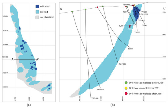
Figure 15.
Visual representation of the results obtained for resource classification in Case Study 4: (a) overhead view of Tom West’s block model; (b) cross-section of the central portion of Tom West’s block model.
4. Discussion
The classical methods traditionally adopted by the industry for resource classification have historically focused on a narrow set of criteria, primarily geometric parameters—such as the number and distance of composites and/or drillholes—and spatial continuity metrics, such as kriging variance. While these elements form the technical foundation of resource classification, relying on them exclusively may result in an incomplete assessment, particularly when critical factors such as data quality and reliability are not incorporated.
As illustrated by the present case study, this limited approach can lead to a misrepresentation of the uncertainty associated with the resource model. Specifically, blocks with low estimation confidence may be mistakenly classified into higher confidence categories, thereby compromising the technical credibility and robustness of the project.
These oversights can have direct and significant consequences in both mine planning and economic evaluation, as they may give rise to technical and financial expectations that do not correspond to the true quality of the estimated resources. For this reason, it is essential to adopt more comprehensive methodologies that integrate geometric, statistical, geometallurgical, and deposit-specific factors, thereby producing a classification framework that is both representative and defensible.
This study presents a comprehensive methodology designed to incorporate complementary parameters into the mineral resource estimation process. The aim is to improve the identification of areas with inherent uncertainty that often remain undetected by conventional techniques used for mineral resource classification. This approach provides a more detailed and robust understanding of the confidence in the resource model. The proposed methodology is distinguished by its simplicity and flexibility, allowing for straightforward implementation and easy scalability across different stages of a mining project and geological contexts. This adaptability ensures that the approach can be tailored to meet the unique requirements and complexities of each case study, thereby enhancing the accuracy and reliability of resource estimates. Furthermore, the methodology is fully compatible with advanced deep-learning techniques (DL), which are capable of generating detailed probability volumes, e.g., [92]. These volumes assign each voxel a probabilistic value that quantifies the degree of confidence associated with the estimation, thus enabling a more informed decision-making process by explicitly addressing uncertainty within the model. This integration of deep-learning methods further enhances the methodology’s capability to produce high-quality, data-driven resource classifications that can better support future exploration campaigns and mine planning.
The integration of diverse criteria—both quantitative and qualitative—is a complex and non-trivial task, requiring systematic and rigorous analysis to ensure internal consistency in the classification process. It is also important to acknowledge that resource classification remains, to a large extent, a subjective exercise, dependent on the professional judgement and criteria applied by the competent person. Therefore, any modifying factors—whether favorable or adverse—must be clearly documented and thoroughly justified, given their substantial influence on the final classification outcome.
Additionally, visual tools such as resource classification maps, sections, and 3D models should be included as a standard practice. Relying solely on tabulated estimates disaggregated by category is insufficient. Visual representations are crucial for evaluating whether the classification reflects coherent geological continuity and avoids artificial patterns or spatial artifacts.
5. Conclusions
This study has highlighted the inherent limitations of traditional mineral resource classification methods. While these approaches form the foundation of classification practices, their isolated application may be insufficient to adequately reflect the full extent of uncertainty associated with the database used in deposit evaluation. This shortcoming can lead to the misclassification of resource categories, particularly in areas characterized by high variability and/or limited informational support, thereby compromising the technical robustness of the resource model.
Consequently, it is imperative to move towards classification methodologies that integrate additional variables, such as geometallurgical criteria, explicit measures of uncertainty, and qualitative aspects of data reliability. Likewise, there is a clear need to enhance the transparency of the classification process through the inclusion of visual representations—such as maps and interpretative sections—that support the reported estimates, moving beyond the conventional reliance on numerical tables alone.
Finally, given the inherently subjective nature of the classification process, it is essential to rigorously document and justify the technical criteria and modifying factors applied, in order to ensure the traceability, reproducibility, and credibility of the results for both the technical community and regulatory authorities.
Author Contributions
Conceptualization, C.C.F., I.D.Á. and G.A.; methodology, C.C.F., I.D.Á., A.K. and G.A.; software, C.C.F. and G.A.; investigation, G.A.; supervision, C.C.F., I.D.Á. and A.K.; visualization, C.C.F. and G.A.; original draft preparation, G.A.; writing—review and editing, G.A., C.C.F., I.D.Á. and A.K. All authors have read and agreed to the published version of the manuscript.
Funding
This research received no external funding.
Data Availability Statement
The data used for the case study presented in this work form part of the Macpas Project database. These data were released by FIREWEED METALS CORP. (https://fireweedmetals.com/macpass-project/, accessed on 25 August 2025). The software employed for the case study were RecMin (https://recmin.com/WP/, accessed on 25 August 2025) and RecMin Variograms (https://recmin.com/WP/?wpdmpro=rm-variograms, accessed on 25 August 2025), both of which are freeware. For further information regarding this work, please contact the authors.
Acknowledgments
We would like to express our sincere gratitude to FIREWEED METALS CORP for providing us with the drillhole information that was necessary for the execution of this study.
Conflicts of Interest
The authors declare no conflicts of interest.
References
- Peters, W.C. Exploration and Mining Geology; John Wiley and Sons Inc.: New York, NY, USA, 1978. [Google Scholar]
- Bárdossy, G.; Fodor, J. Traditional and new ways to handle uncertainty in geology. Nat. Resour. Res. 2001, 10, 179–187. [Google Scholar] [CrossRef]
- Dominy, S.C.; Noppé, M.A.; Annels, A.E. Errors and uncertainty in mineral resource and ore reserve estimation: The importance of getting it right. Explor. Min. Geol. 2002, 11, 77–98. [Google Scholar] [CrossRef]
- Rossi, M.E.; Deutsch, C.V. Mineral Resource Estimation; Springer Science & Business Media: Heidelberg, Germany, 2013. [Google Scholar]
- Konieczka, P. The role of and the place of method validation in the quality assurance and quality control (QA/QC) system. Crit. Rev. Anal. Chem. 2007, 37, 173–190. [Google Scholar] [CrossRef]
- Wellmer, F.W.; Dalheimer, M.; Wagner, M. Economic Evaluations in Exploration; Springer Science & Business Media: Heidelberg, Germany, 2007. [Google Scholar]
- Jones, I.O.; Aspandiar, M.; Dugdale, A.; Leggo, N.; Glacken, I.; Smith, B. The Business of Mining: Mineral Deposits, Exploration and Ore-Reserve Estimation; CRC Press: Boca Raton, FL, USA, 2019; Volume 3. [Google Scholar]
- McManus, S.; Rahman, A.; Coombes, J.; Horta, A. Uncertainty assessment of spatial domain models in early stage mining projects—A review. Ore Geol. Rev. 2021, 133, 104098. [Google Scholar] [CrossRef]
- Schindler, C.; Hagemann, S.; Banks, D.; Mernagh, T.; Harris, A. Magmatic hydrothermal fluids at the sedimentary rock-hosted, intrusion-related Telfer gold-copper deposit, Paterson Orogen, Western Australia: Pressure-temperature-composition constraints on the ore-forming fluids. Econ. Geol. 2016, 111, 1099–1126. [Google Scholar] [CrossRef]
- Newcrest Mining Limited. Concise Annual Report 2003. 2003. Available online: https://www.annualreports.com/HostedData/AnnualReportArchive/N/ASX_NCM_2003.pdf (accessed on 25 August 2025).
- Newcrest Mining Limited. Concise Annual Report 2006. 2006. Available online: https://www.annualreports.com/HostedData/AnnualReportArchive/N/ASX_NCM_2006.pdf (accessed on 25 August 2025).
- Newcrest Mining Limited. Concise Annual Report 2007. 2007. Available online: https://www.annualreports.com/HostedData/AnnualReportArchive/N/ASX_NCM_2007.pdf (accessed on 25 August 2025).
- Carlson, R. Understanding geologic uncertainty in mining studies. SEG Newsl. 2019, 117, 21–29. [Google Scholar] [CrossRef]
- Hall, W.S. Geology and Paragenesis of the Boseto Copper Deposits, Kalahari Copperbelt, Northwest Botswana; Colorado School of Mines: Golden, CO, USA, 2013. [Google Scholar]
- Discovery Metals Limited. Australian Securities Exchange (ASX) Conference. Conference Presentation, London. 2012. Available online: https://announcements.asx.com.au/asxpdf/20120427/pdf/425vrvp0bw43zx.pdf (accessed on 25 August 2025).
- King, H.F. Guide to the Understanding of Ore Reserve Estimation; The Australasian Institute of mining and Metallurgy: Parkville, VIC, Australia, 1982; Available online: https://www.jorc.org/docs/historical_documents/kng_mcmahon1982.pdf (accessed on 25 August 2025).
- Gallagher, S.; Camacho, A.; Fayek, M.; Epp, M.; Spell, T.L.; Armstrong, R. Geology, geochemistry, and geochronology of the East Bay gold trend, Red Lake, Ontario, Canada. Miner. Depos. 2018, 53, 127–141. [Google Scholar] [CrossRef]
- SRK Consulting (Canada) Inc.; Rubicon Minerals Corporation. Preliminary Economic Assessment for the F2 Gold System, Phoenix Gold Project, Red Lake, Ontario. Technical Report. 2013. Available online: https://digigeodatareports.b-cdn.net/3443.pdf (accessed on 25 August 2025).
- SRK Consulting (Canada) Inc.; Rubicon Minerals Corporation. Technical Report for the Phoenix Gold Project, Red Lake, Ontario. Technical Report. 2016. Available online: https://www.sedarplus.ca/csfsprod/data153/filings/02447061/00000001/C%3A%5CSEDAR%5CFILINGS%5CTechnicalReport%5CTechReport.pdf (accessed on 25 August 2025).
- Rubicon Minerals Corporation, Golden Associates Ltd. National Instrument 43-101 Technical Report for the Rubicon Phoenix Gold Project. Technical Report. 2018. Available online: https://digigeodatareports.b-cdn.net/415.pdf (accessed on 25 August 2025).
- Gold, B.N. Corp. National Instrument 43-101 Technical Report Bateman Gold Project: F2 Gold Deposit Feasibility Study and McFinley Zone Mineral Resource Estimate, Cochenour, Ontario.Technical Report. 2021. Available online: https://s28.q4cdn.com/583965976/files/doc_multimedia/portfolios/bateman-gold-project-technical-report-january-27-2021.pdf (accessed on 25 August 2025).
- Lindi, O.T.; Aladejare, A.E.; Ozoji, T.M.; Ranta, J.P. Uncertainty quantification in mineral resource estimation. Nat. Resour. Res. 2024, 33, 2503–2526. [Google Scholar] [CrossRef]
- Silva, D.; Boisvert, J. Mineral resource classification: A comparison of new and existing techniques. J. S. Afr. Inst. Min. Metall. 2014, 114, 265–273. [Google Scholar]
- Sadeghi, B.; Madani, N.; Carranza, E.J.M. Combination of geostatistical simulation and fractal modeling for mineral resource classification. J. Geochem. Explor. 2015, 149, 59–73. [Google Scholar] [CrossRef]
- Yasrebi, A.B.; Hezarkhani, A. Resources classification using fractal modelling in Eastern Kahang Cu-Mo porphyry deposit, Central Iran. Iran. J. Earth Sci. 2019, 11, 56–67. [Google Scholar]
- Afzal, P.; Gholami, H.; Madani, N.; Yasrebi, A.B.; Sadeghi, B. Mineral resource classification using geostatistical and fractal simulation in the Masjed Daghi Cu–Mo porphyry deposit, NW Iran. Minerals 2023, 13, 370. [Google Scholar] [CrossRef]
- Hernández, H. A semiautomatic multi criteria method for mineral resources classification. Appl. Earth Sci. 2024, 133, 211–223. [Google Scholar] [CrossRef]
- Nwaila, G.T.; Carranza, E.J.M. Uncertainty Quantification of Microblock-Based Resource Models and Sequencing of Sampling. Nat. Resour. Res. 2025, 34, 1927–1952. [Google Scholar] [CrossRef]
- Lehman, J.A. The Bre-X Stock Debacle: Why the Enactment of Canadian Federal Securities Legislation Would be Good as Gold. Brook. J. Int’l L. 1998, 24, 823. [Google Scholar]
- Drozdiak, J. Bre-X, NI 43-101 and the effectiveness of regulating mineral project disclosure in Canada. Can. Bus. LJ 2017, 60, 343. [Google Scholar]
- Rendu, J.; Miskelly, N. Mineral resources and mineral reserves: Progress on international definitions and reporting standards. Min. Technol. 2001, 110, 133–138. [Google Scholar] [CrossRef]
- Miskelly, N. Progress on international standards for reporting of mineral resources and reserves. In Proceedings of the Conference on Resource Reporting Standards, Reston, VA, USA, 20–22 October 2003; Volume 3, pp. 1–22. [Google Scholar]
- JORC Committee. The JORC Code 2012 Edition, Joint Ore Reserves Committee of the Australasian Institute of Mining and Metallurgy, Australian Institute of Geoscientists and Minerals Council of Australia. 2012. Available online: https://www.jorc.org/docs/JORC_code_2012.pdf (accessed on 25 August 2025).
- CSA. National Instrument 43-101 Standards of Disclosure for Mineral Projects. 2011. Available online: https://mrmr.cim.org/media/1017/national-instrument-43-101.pdf (accessed on 25 August 2025).
- GSSA. The South African Code for the Reporting of Exploration Results, Mineral Resources and Mineral Reserves; 2016 Edition. 2016. Available online: https://mrmr.cim.org/media/1049/515-samrec_2016.pdf (accessed on 25 August 2025).
- SME. The SME Guide for Reporting Exploration Results, Mineral Resources and Mineral Reserves. 2017. Available online: https://smenet.blob.core.windows.net/smecms/sme/media/smeazurestorage/professional%20development/pdf%20files/smeguidereporting_082017.pdf (accessed on 25 August 2025).
- PERC. PERC Reporting Standard 2013, Pan-European Standard for Reporting of Exploration Results, Mineral Resources and Reserves. 2013. Available online: https://percstandard.org/wp-content/uploads/2021/06/PERC_REPORTING_STANDARD_2013.pdf (accessed on 25 August 2025).
- USGS. Principles of a Resource/Reserve Classification for Minerals: U.S. Geological Survey Circular 831. 1980. Available online: https://pubs.usgs.gov/circ/1980/0831/report.pdf (accessed on 25 August 2025).
- CRIRSCO. International Reporting Template for the Public Reporting of Exploration Targets, Exploration Results, Mineral Resources and Mineral Reserves. 2024. Available online: https://crirsco.com/wp-content/uploads/2023/10/The-CRIRSCO-International-Reporting-Template.pdf (accessed on 25 August 2025).
- Stephenson, P. Mineral Resource Classification: How the Viability of Your Project May Hang on a Qualified Person’s Judgement; Technical report; Canadian Institute of Mining, Metallurgy and Petroleum: Westmount, QC, Canada, 2011. [Google Scholar]
- Battalgazy, N.; Madani, N. Categorization of mineral resources based on different geostatistical simulation algorithms: A case study from an iron ore deposit. Nat. Resour. Res. 2019, 28, 1329–1351. [Google Scholar] [CrossRef]
- CBRR. The CBBR Guide for Reporting Exploration Results, Mineral Resources, and Mineral Reserves. 2016. Available online: https://mrmr.cim.org/media/1054/519-cbrr_2016.pdf (accessed on 25 August 2025).
- Mining Commission for the Qualification of Competencies in Mineral Resources and Mineral Reserves. Code for Reporting of Exploration Results, Mineral Resources and Mineral Reserves. 2015. Available online: https://mrmr.cim.org/media/1046/512-codigo_ingles_2015.pdf (accessed on 25 August 2025).
- CCRR. Colombian Standard for the Public Reporting of Exploration Results, Mineral Resources and Reserves. 2018. Available online: https://mrmr.cim.org/media/1082/colombia-ccrr-reporting-standards-july2018.pdf (accessed on 25 August 2025).
- NAEN. Russian Code for the Public Reporting of Exploration Results, Mineral Resources and Mineral Reserves. 2011. Available online: https://mrmr.cim.org/media/1050/517-naen-2011.pdf (accessed on 25 August 2025).
- KAZRC Association. 34. The Kazakhstan Public Reporting Code for Exploration Results, Mineral Resources and Mineral Reserves. 2016. Available online: https://kazrc.kz/wp-content/uploads/2021/08/KAZRC.pdf (accessed on 25 August 2025).
- MRC. Mongolian Code for the Public Reporting of Exploration Results, Mineral Resources and Mineral Reserves. 2014. Available online: https://mrmr.cim.org/media/1053/518-mrc-2014.pdf (accessed on 25 August 2025).
- UMREK. The National Public Reporting of Exploration Results, Mineral Resources and Mineral Reserves Code of Turkey. 2018. Available online: https://crirsco.com/wp-content/uploads/2023/12/TURKEY-UMREK-2023-English.pdf (accessed on 25 August 2025).
- NACRI. Indian Mineral Industry Code. 2019. Available online: https://mrmr.cim.org/media/1176/imic_july_2019.pdf (accessed on 25 August 2025).
- KCMI. Exploration Results, Mineral Resources and Mineral Reserves (KODE – KCMI). 2017. Available online: https://mrmr.cim.org/media/1051/5111-kcmi-code-2017.pdf (accessed on 25 August 2025).
- Deutsch, C.V.; Leuangthong, O.; Ortiz, J. Case for geometric criteria in resources and reserves classification. Trans.-Soc. Min. Metall. Explor. Inc. 2007, 322, 104098. [Google Scholar]
- Nowak, M.; Leuangthong, O. Optimal drill hole spacing for resource classification. In Mining Goes Digital; CRC Press: Boca Raton, FL, USA, 2019; pp. 115–124. [Google Scholar]
- Glacken, I.; Rondon, O.; Levett, J. Drill Hole Spacing Analysis for Classification and Cost Optimisation—A Critical Review of Techniques. In Proceedings of the Mineral Resource Estimation Conference 2023, Melbourne, Australia, 24–25 May 2023; pp. 179–191. [Google Scholar]
- Blackwell, G. Relative kriging errors: A basis for mineral resource classification. Explor. Min. Geol. 1998, 7, 99–105. [Google Scholar]
- Sinclair, A.; Blackwell, G. Resource/reserve classification and the qualified person. CIM Bull. 2000, 93, 29–35. [Google Scholar]
- Souza, L.; Costa, J.; Koppe, J. A geostatistical contribution to assess the risk embedded in resource classification methods. In Proceedings of the Iron Ore Conference, Perth, Australia, 27–29 July 2009. [Google Scholar]
- Rivoirard, J.; Renard, D.; Celhay, F.; Benado, D.; Queiroz, C.; Oliveira, L.J.; Ribeiro, D. From the spatial sampling of a deposit to mineral resources classification. In Geostatistics Valencia 2016; Springer: Heidelberg, Germany, 2017; pp. 329–344. [Google Scholar]
- Wawruch, T.M.; Betzhold, J.F. Mineral resource classification through conditional simulation. In Geostatistics Banff 2004; Springer: Heidelberg, Germany, 2005; pp. 479–489. [Google Scholar]
- Emery, X.; Maleki, M. Geostatistics in the presence of geological boundaries: Application to mineral resources modeling. Ore Geol. Rev. 2019, 114, 103124. [Google Scholar] [CrossRef]
- Madenova, Y.; Madani, N. Application of Gaussian mixture model and geostatistical co-simulation for resource modeling of geometallurgical variables. Nat. Resour. Res. 2021, 30, 1199–1228. [Google Scholar] [CrossRef]
- Verly, G.; Parker, H.M. Conditional simulation for mineral resource classification and mining dilution assessment from the early 1990s to now. Math. Geosci. 2021, 53, 279–300. [Google Scholar] [CrossRef]
- Owusu, S.; Dagdelen, K. Critical review of mineral resource classification techniques in the gold mining industry. Min. Goes Digit. 2019, 201–209. [Google Scholar]
- País Cerna, G.E. Definición de un Nuevo Criterio de Categorización de Recursos Minerales Basado en Simulaciones Geoestadísticas. Master’s Thesis, Universidad de Chile, Santiago, Chile, 2021. Available online: https://repositorio.uchile.cl/bitstream/handle/2250/181874/Definicion-de-un-nuevo-criterio-de-categorizacion-de-recursos-minerales-basado-en-simulaciones-geoestadisticas.pdf?sequence=1&isAllowed=y (accessed on 25 August 2025).
- Diehl, P.; David, M. Classification of ore reserves/resources based on geostatistical methods. CIM Bull. 1982, 75, 77–83. [Google Scholar]
- Froidevaux, R. Geostatistics and ore reserve classification. CIM Bull. 1982, 75, 77–83. [Google Scholar]
- Royle, A. How to Use Geostatistics for Ore Reserve Classification. Eng. Min. J. 1977, 30, 52–56. [Google Scholar]
- Arik, A. An alternative approach to resource classification. In Proceedings of the International symposium on computer applications in the mineral industries (APCOM’99), Golden, CO, USA, 20–22 October 1999; Volume 28, pp. 45–53. [Google Scholar]
- Journel, A. Geostatistics: Models and tools for the earth sciences. Math. Geol. 1986, 18, 119–140. [Google Scholar] [CrossRef]
- Isaaks, E.H.; Srivastava, R.M. Applied Geostatistics; Oxford University Press: New York, NY, USA, 1989. [Google Scholar]
- Yamamoto, J.K. Quantification of uncertainty in ore-reserve estimation: Applications to Chapada copper deposit, State of Goiás, Brazil. Nat. Resour. Res. 1999, 8, 153–163. [Google Scholar] [CrossRef]
- Sabourin, R.L. Application of a geostatistical method to quantitatively define various categories of resources. In Geostatistics for Natural Resources Characterization: Part 1; Springer: Heidelberg, Germany, 1984; pp. 201–215. [Google Scholar]
- Froidevaux, R.; Roscoe, W.; Valiant, R. Estimating and classifying gold reserves at Page-Williams C zone: A case study in nonparametric geostatistics. In Proceedings of the Proceedings of the Symposium on Ore Reserve Estimation—Methods, Models and Reality: Canadian Institute of Mining, Metallurgy and Petroleum, Montreal, QC, Canada, 10–11 May 1986; pp. 280–300. [Google Scholar]
- Snowden, D. Practical interpretation of mineral resource and ore reserve classification guidelines. In Mineral Resource and Ore Reserve Estimation—The AusIMM Guide to Good Practice; Australasian Institute of Mining and Metallurgy: Carlton, VIC, Australia, 2001; pp. 643–652. [Google Scholar]
- Emery, X.; Ortiz, J.M.; Rodríguez, J.J. Quantifying uncertainty in mineral resources by use of classification schemes and conditional simulations. Math. Geol. 2006, 38, 445–464. [Google Scholar] [CrossRef]
- Dohm, C. Quantifiable mineral resource classification: A logical approach. In Geostatistics Banff 2004; Springer: Heidelberg, Germany, 2004; pp. 333–342. [Google Scholar]
- Annels, A.; Dominy, S. Core recovery and quality: Important factors in mineral resource estimation. Appl. Earth Sci. 2003, 112, 305–312. [Google Scholar] [CrossRef]
- Bieniawski, Z. Engineering classification of jointed rock masses. Civ. Eng. Siviele Ingenieurswese 1973, 1973, 335–343. [Google Scholar]
- Bieniawski, Z.T. Rock Mechanics Design in Mining and Tunneling; A.A. Balkema: Rotterdam, The Netherlands, 1984. [Google Scholar]
- Bieniawski, Z.T. Engineering Rock Mass Classifications: A Complete Manual for Engineers and Geologists in Mining, Civil, and Petroleum Engineering; John Wiley & Sons: Hoboken, HJ, USA, 1989. [Google Scholar]
- Barton, N.; Lien, R.; Lunde, J. Engineering classification of rock masses for the design of tunnel support. Rock Mech. 1974, 6, 189–236. [Google Scholar] [CrossRef]
- Barton, N.; Lien, R.; Lunde, J. Estimation of support requirements for underground excavations. In Proceedings of the ARMA US Rock Mechanics/Geomechanics Symposium. ARMA, Minneapolis, MN, USA, 22–24 September 1975; p. ARMA–75. [Google Scholar]
- Grimstad, E.d. Updating the Q-system for NMT. In Proceedings of the International Symposium on Sprayed Concrete-Modern Use of Wet Mix Sprayed Concrete for Underground Support, Norwegian Concrete Association, Fagemes, Oslo, Norway, 22–26 October 1993; pp. 46–66. [Google Scholar]
- Palmstrom, A.; Broch, E. Use and misuse of rock mass classification systems with particular reference to the Q-system. Tunn. Undergr. Space Technol. 2006, 21, 575–593. [Google Scholar] [CrossRef]
- Sternesky, M. Exploration process optimization: A vision for the integrated exploration workflow. First Break 2010, 28, 79–83. [Google Scholar] [CrossRef]
- de Kemp, E.A.; Schetselaar, E.M.; Hillier, M.J.; Lydon, J.W.; Ransom, P.W. Assessing the workflow for regional-scale 3D geologic modeling: An example from the Sullivan time horizon, Purcell Anticlinorium East Kootenay region, southeastern British Columbia. Interpretation 2016, 4, SM33–SM50. [Google Scholar] [CrossRef][Green Version]
- RecMin. RecMin: Mining Sofware. 2025. Available online: https://recmin.com/WP/ (accessed on 25 August 2025).
- RecMin. RecMin Variograms. 2025. Available online: https://recmin.com/WP/?wpdmpro=rm-variograms/ (accessed on 25 August 2025).
- Buelga Díaz, A.; Castañón Fernández, C.; Ares, G.; Prieto, D.A.; Álvarez, I.D. RecMin Variograms: Visualisation and Three-Dimensional Calculation of Variograms in Block Modelling Applications in Geology and Mining. Int. J. Environ. Res. Public Health 2022, 19, 12454. [Google Scholar] [CrossRef]
- Goodfellow, W.D.; Lydon, J.W.; Turner, R.J.W. Geology and genesis of stratiform sediment-hosted (SEDEX) zinc-lead-silver sulphide deposits. In Geological Association of Canada, Special Paper; Geological Association of Canada: St. John’s, NL, Canada, 1993; Volume 40, pp. 201–251. [Google Scholar]
- Goodfellow, W. Base metal metallogeny of the Selwyn Basin, Canada. In Mineral Deposits of Canada: A Synthesis of Major Deposit-Types, District Metallogeny, the Evolution of Geological Provinces, and Exploration Methods; Geological Association of Canada, Mineral Deposits Division, Special Publication: St. John’s, NL, Canada, 2007; Volume 5, pp. 553–579. [Google Scholar]
- Corp, F.M. Macpass Project Data. 2025. Available online: https://fireweedmetals.com/macpass-project/ (accessed on 1 July 2025).
- Zhang, B.; Xu, K.; Khan, U.; Li, X.; Du, L.; Xu, Z. A lightweight convolutional neural network with end-to-end learning for three-dimensional mineral prospectivity modeling: A case study of the Sanhetun Area, Heilongjiang Province, Northeastern China. Ore Geol. Rev. 2023, 163, 105788. [Google Scholar] [CrossRef]


Disclaimer/Publisher’s Note: The statements, opinions and data contained in all publications are solely those of the individual author(s) and contributor(s) and not of MDPI and/or the editor(s). MDPI and/or the editor(s) disclaim responsibility for any injury to people or property resulting from any ideas, methods, instructions or products referred to in the content. |
© 2025 by the authors. Licensee MDPI, Basel, Switzerland. This article is an open access article distributed under the terms and conditions of the Creative Commons Attribution (CC BY) license (https://creativecommons.org/licenses/by/4.0/).