Modulation Recognition Algorithm for Long-Sequence, High-Order Modulated Signals Based on Mamba Architecture

Abstract

This paper investigates modulation recognition technology for high-order modulated signals. Addressing the issue that existing deep learning-based modulation recognition methods struggle to effectively capture the features of long sequence signals in high-order modulation, we propose a ConvMamba model that integrates convolutional neural networks (CNNs) with the Mamba2 architecture. By employing a selective state-space model, the ConvMamba effectively captures the temporal dependencies in long sequence signals. It also combines the local feature extraction capability of CNNs with a soft-thresholding denoising module, forming a hybrid structure that possesses both global modeling and noise resistance capabilities. The evaluation results on the Sig53 dataset, which contains a rich variety of high-order modulations, demonstrate that compared to traditional CNN- or Transformer-based architectures, ConvMamba achieves a better balance between computational efficiency and recognition accuracy. Compared to Transformer models with similar performance, ConvMamba reduces computational complexity by over 60%. Compared to CNN models with comparable computational resource consumption, ConvMamba significantly improves recognition accuracy. Therefore, ConvMamba shows a distinct advantage in processing high-order modulated signals with long sequences.

1. Introduction

Automatic modulation recognition (AMR), also referred to as adaptive modulation recognition, has found widespread applications in areas such as adaptive communication, cognitive radio, and spectrum monitoring. Since its introduction, it has garnered extensive attention and undergone in-depth research [1,2,3]. In recent years, with the rapid and groundbreaking advancements in the field of deep learning, research on deep learning-based AMR (DL-AMR) has also achieved rapid development [4]. With the construction of multi-layer neural networks, DL-AMR is capable of automatically learning and extracting complex features from modulated signals, thereby significantly improving recognition performance. To date, the academic community has extensively studied DL-AMR techniques and proposed a series of highly effective model approaches. These include convolutional neural networks (CNNs) [5], recurrent neural networks (RNNs) [6], autoencoders [7], transformers [8], as well as various hybrid architectures [9,10,11]. In addition, a number of effective methods have been proposed in the area of signal preprocessing, involving techniques such as cyclic correntropy spectra [12], time-frequency analysis [13], and polar coordinate representations [14]. At the same time, with the rapid advancement of communication technologies, higher-order modulations—such as 512-QAM and 1024-QAM—are increasingly being adopted in systems like 5G [15], Wi-Fi 7 [16], and Power Line Communication (PLC) systems [17]. While these high-order modulations significantly enhance data transmission rates and spectral efficiency, they also pose substantial challenges to AMR research and application. These challenges are mainly reflected in three aspects: First, the constellation diagrams of high-order modulations are denser, and the signal features are more complex, making it difficult for traditional deep learning methods to effectively extract discriminative features. Second, high-order modulations have lower tolerance to channel noise and interference, meaning that the impact of signal distortion becomes more pronounced. Third, the recognition of high-order modulations often requires longer sequences of signal data. Traditional deep learning models struggle to effectively capture long-range temporal dependencies, and longer sequences also lead to significantly increased computational demands. As a result, deep learning-based modulation recognition for high-order modulation and long-sequence signals has emerged as a research hotspot in the AMR field. This is precisely the focus of the current study. Below, we provide a brief overview of the current domestic and international research status in this area.

Recently, researchers have carried out preliminary studies on modulation recognition of long-sequence signals with high-order modulation [18,19,20,21,22,23]. Xu et al. [18] proposes a DL-AMR algorithm for orthogonal frequency division multiplexing systems based on orthogonal space-time block coding and high-order modulation. It first uses blind zero-forcing equalization to reconstruct damaged signals to enhance signal representation ability then introduces a constellation accumulation strategy to generate accumulated constellation diagrams to reduce constellation point dispersion; finally, it uses constellation temporal convolution instead of traditional two-dimensional convolution to reduce computational overhead and extract more discriminative features. Experimental results show that this method performs excellently on 14 modulation signals. To address the training and storage overhead issues caused by long-sequence signals, Zhang et al. [19] introduced a selective state-space model as the backbone network, achieving efficient recognition of long-sequence signals by reducing the dimension of the state matrix. To solve the problem of poor recognition performance of existing methods under low signal-to-noise ratio conditions, He et al. [20] designed a DL-AMR model based on feature fusion and multi-core classifier, which uses convolution and gated recurrent units to extract deep features of high-order modulated signals and adopted high-order cumulants as supplementary features, effectively improving the recognition accuracy of high-order modulation under low signal-to-noise ratio conditions. To promote the development of DL-based high-order modulation recognition technology, Boegner et al. [21] first constructed a Sig53 dataset containing various high-order modulation types and released the wireless communication toolbox torchSig, enabling researchers to customize various modulated signals and impairments. On this basis, the authors designed modulation classification methods based on CNN and Transformer models as research benchmarks for the Sig53 dataset. Experimental results show that the Transformer demonstrates unique advantages in capturing long temporal dependencies by virtue of its self-attention mechanism, providing new ideas for in-depth understanding of long-sequence signal features. Cai et al. [22] first applied the Transformer to AMR, which divides long I/Q sequences into multiple equal-length short sequences and feeds them into the network, showing excellent performance compared with traditional CNN and LSTM models. Ma et al. [23] proposes a parallel CNN–Transformer structure, utilizing the advantages of the Transformer in capturing long-distance dependencies of signals and the ability of convolutional networks to extract local information simultaneously. The experimental results show that this design can improve recognition accuracy.

Although current researchers have carried out preliminary studies on modulation recognition of long-sequence signals with high-order modulation, the methods proposed in existing studies still have some shortcomings: The proposed CNN-based models, although excellent in local feature extraction, have limited ability to capture global information and struggle to effectively capture long-range temporal dependencies in signals. The Transformer architecture effectively models global information through a self-attention mechanism, but its computational complexity is quadratic with sequence length, and it faces huge computational resource consumption when processing long sequences. To this end, this research studied modulation recognition technology for high-order modulated long-sequence signals and proposes a DL-AMR method based on the Mamba2 architecture. By fusing Mamba2 and CNN structures, a hybrid network model with long time dependency modeling capability was constructed, thereby overcoming the dilemma of insufficient accuracy or high computational complexity faced by existing recognition methods in processing long-sequence signals. The main contributions of this study can be summarized as follows:

(1)

Based on an in-depth analysis of the impact of long-sequence, high-order modulated signals on DL-AMR tasks, a hybrid architecture model named ConvMamba is proposed. This model cleverly combines the local feature extraction capability of a CNN with the long-sequence modeling capability of Mamba2 [24], constructing an efficient network model that can effectively capture long time dependencies.

(2)

Due to its soft-threshold denoising algorithm, the model can maintain more stable recognition performance in various complex environments, improving the robustness of the model; further, a feature fusion module is introduced into the model for sequence dimensionality reduction, achieving hierarchical feature representation and improving computational efficiency.

(3)

Experimental validation of the proposed model method was conducted on the Sig53 dataset. The results indicate that compared with traditional CNN-based models, ConvMamba achieves higher recognition accuracy while significantly reducing computational and storage requirements compared to Transformer-based models.

The remaining parts of this paper are structured as follows: Section 2 introduces the AMR signal model and DL-AMR method framework; Section 3 elaborates on the proposed ConvMamba model and its functional modules; Section 4 introduces the experimental dataset, experimental process, and results analysis; and Section 5 concludes the paper.

2. AMR Signal Model and DL-AMR Method Framework

2.1. AMR Signal Model

In AMR research, a typical transmitted signal model is

$$x\left(t\right)=\sum _{n=0}^{N}s\left[n\right]g(t-nT),$$

(1)

where $s\left[n\right]$ is the modulated symbol mapped to the complex plane, T is the symbol period, N is the number of symbols, and $g(·)$ represents a shaping pulse (e.g., a raised cosine filter). The orthogonal decomposition of $x\left(t\right)$ is defined as $x\left(t\right)=I\left(t\right)+jQ\left(t\right)$, where $I\left(t\right)=\mathrm{Re}\left[x\right(t\left)\right]$ is the in-phase component and $Q\left(t\right)=\mathrm{Im}\left[x\right(t\left)\right]$ is the quadrature component. The passband transmission signal obtained after carrier modulation of the baseband signal is

$$x_T\left(t\right)=\mathrm{Re}\left\{x\left(t\right)e^{j{\omega }_{c}t}\right\}=I\left(t\right)cos\left({\omega }_{c}t\right)-Q\left(t\right)sin\left({\omega }_{c}t\right),$$

(2)

where ${\omega }_c=2\pi f_c$ and $f_c$ is the carrier frequency.

The transmitted signal reaches the receiver through the channel. Due to various non-ideal hardware effects at the transceiver (including power amplifier nonlinearity, I/Q imbalance, phase noise, etc.) and channel fading effects, the signal received by the receiver has frequency, phase, and timing offsets, as well as amplitude fading [25]. After down-conversion at the receiver, the received equivalent baseband signal can be expressed as:

$$r\left(t\right)=h\left(t\right)\ast x_T\left(t\right)e^{j(2\pi \Delta ft+\theta )}+n\left(t\right),$$

(3)

where $h\left(t\right)$ denotes the channel impulse response, ∗ denotes convolution, $\Delta f$ is the carrier frequency offset, $\theta$ is the phase offset, and $n\left(t\right)$ is additive white Gaussian noise.

2.2. DL-AMR Basic Framework

DL-AMR tasks are usually constructed as a supervised learning problem, whose core goal is to accurately determine the modulation type $m\in \mathcal{M}$ of the transmitted signal by analyzing the signal $r\left(t\right)$ obtained at the receiver, where $\mathcal{M}=\{m_1,m_2,...,m_M\}$ represents the set of all possible modulation types, and $\mathcal{M}$ is the total number of categories. As shown in Figure 1, a typical DL-AMR system usually includes the following steps: first, the received original signal undergoes feature preprocessing (such as time-frequency analysis, denoising, etc.) to obtain a feature representation $\mathbf{X}$ suitable for network recognition. The preprocessed signal is input into a deep neural network for feature extraction, which can be expressed as $\mathbf{Z}=g_{\theta }\left(\mathbf{X}\right)$, where $g_{\theta }(·)$ is the feature extraction sub-network and $\mathbf{Z}$ is the extracted discriminative feature. Finally, the extracted features are fed into a classifier, which outputs a probability distribution representing the probability that the input signal belongs to each possible modulation type:

$$\mathbf{p}=\mathrm{softmax}(\mathbf{WZ}+\mathbf{b}),$$

(4)

where $\mathbf{W}$ and $\mathbf{b}$ are the weight matrix and bias vector of the classifier, respectively; $\mathrm{softmax}(·)$ is a commonly used output layer in deep learning models, which maps the final feature representation to a probability distribution; $\mathbf{p}={[p_1,p_2,\dots ,p_j,\dots ,p_M]}^T$ represents the probability that the signal belongs to each modulation type. The modulation mode $\widehat{m}$ predicted by the model is

$$\widehat{m}=\underset{m_j\in \mathcal{M}}{argmax}{p}_j.$$

(5)

The training process of the deep learning model is realized by minimizing the loss function $L\left(\theta \right)$ with respect to the model parameters $\theta$ on the training dataset. In this paper, cross-entropy loss is used, defined as

$$L\left(\theta \right)=-{\displaystyle \frac{1}{S}}\sum _{i=1}^S\sum _{j=1}^{M}1\left(m_i=m_j\right)log{p}_{ij},$$

(6)

where $1(m_i=m_j)$ is an indicator function, which indicates whether the true label of sample i is $m_j$, S is the total number of samples, and $p_{ij}$ is the predicted probability that the i-th sample belongs to the j-th class. The training process usually uses gradient descent (e.g., SGD, Adam) to iteratively update parameters $\theta$ to minimize the loss function $L\left(\theta \right)$:

$${\theta }^{\ast }=arg\underset{\theta }{min}L\left(\theta \right).$$

(7)

3. ConvMamba Model Design

As mentioned earlier, in the modulation recognition of high-order modulated long-sequence signals, the key is to extract and recognize the long-range temporal dependency features of signal sequences without significantly increasing model resource overhead. To this end, this section proposes the ConvMamba architecture, which integrates CNN and Mamba2 architectures, leveraging the advantages of a CNN in local feature extraction and Mamba2 in long-sequence modeling. The overall architecture of the model and the specific implementation of each key module are elaborated below.

3.1. Overall Model Structure

The overall architecture of the proposed ConvMamba model for high-order modulated signal recognition is shown in Figure 2. The model consists of key components: a convolutional layer (Conv 1D), a soft-threshold denoising module (Denoising), a CNN–Mamba2 hybrid structure (Stage-1 to Stage-4), a feature fusion module (Patch Merging), and a feature classifier (Classifier).

The processing flow of the model can be divided into four main stages: first, the input I/Q signal is initially processed through a convolutional structure, and the signal channel dimension is adjusted using linear mapping to obtain initial features ${\mathbf{X}}_s\in {\mathbb{R}}^{{\displaystyle \frac{L}{S}}\times C}$ (where S is the convolution stride, C is the adjusted number of channels, and L is the length of the input signal). Then, the signal is processed through a soft-threshold denoising module, which can effectively suppress additive noise in the communication channel, improve the anti-noise ability and robustness of the model, and obtain features ${\mathbf{X}}_D\in {\mathbb{R}}^{{\displaystyle \frac{L}{S}}\times C}$. Next, the first stage is constructed by repeatedly stacking CNN–Mamba2 hybrid modules. The CNN–Mamba2 block extracts global information and local features of the signal through a dual-branch structure, constructing deep discriminative information while keeping the feature dimension unchanged. Further, a feature fusion module is introduced to deeply fuse information from different branches of the CNN–Mamba2 model and implement dimensionality reduction to build a hierarchical feature representation. This hierarchical structure helps the model gradually understand the transformation from low-level modulation features to high-level modulation types; afterward, in the second, third, and fourth processing stages, the model repeats the above feature extraction and fusion process and finally outputs a highly abstract feature representation. The output feature after feature fusion at the i-th level can be expressed as ${\mathbf{X}}_i\in {\mathbb{R}}^{{\displaystyle \frac{L}{2^{i}S}}\times 2^{i}C}$. The end of the network uses a classifier composed of an adaptive global average pooling (GAP) layer and a linear layer to complete the recognition of the input signal’s modulation type. The entire model training uses the cross-entropy loss function. The specific training methods and model hyperparameter settings are given in Section 4.

The specific implementations of the core functional modules of the ConvMamba model—namely, the soft-thresholding denoising module, sequence downsampling module, and CNN–Mamba2 hybrid architecture—will be elaborated sequentially below.

3.2. Soft-Threshold Denoising

Extracting modulated signal features in low signal-to-noise ratio environments is extremely challenging, which directly affects the performance of AMR models. To solve this problem, a soft-threshold-based feature optimization strategy is introduced into the proposed ConvMamba model, which effectively attenuates noise components by suppressing features with smaller eigenvalues. Specifically, the soft-threshold function is as follows [6]:

$$y=\left\{\begin{array}{cc}x+sign\left(x\right)\tau \hfill & \mathrm{if}\left|x\right|>\tau \hfill \\ 0\hfill & \mathrm{if}\left|x\right|\le \tau \hfill \end{array}\right.,$$

(8)

where x is the input feature value, $\tau$ is the threshold, and y is the output feature value. This function sets feature values close to zero while retaining negative features containing information, achieving noise suppression. In addition, the derivative of this function has piecewise constant characteristics:

$${\displaystyle \frac{\partial y}{\partial x}}=\left\{\begin{array}{cc}1\hfill & \mathrm{if}\left|x\right|>\tau \hfill \\ 0\hfill & \mathrm{if}\left|x\right|\le \tau \hfill \end{array}\right.,$$

(9)

This piecewise constant derivative characteristic provides numerical stability guarantees for deep network training and can effectively alleviate problems such as gradient vanishing and explosion.

The soft-threshold denoising unit reduces noise interference and enhances the model’s attention to useful information. However, due to the dynamic changes in signal feature distribution and noise environment, it is difficult to determine the optimal threshold. To this end, the model uses an adaptive threshold learning method by referring to the theoretical framework of deep residual shrinkage networks [26]. As shown in Figure 3, for the output features of the convolutional layer in the ConvMamba model, first, two fully connected layers are used to obtain the feature map ${\mathbf{X}}_s$; then, the soft-threshold denoising unit performs absolute value transformation on ${\mathbf{X}}_s$ to ensure the threshold is non-negative. Here, the soft-threshold denoising unit first compresses the feature dimension through the GAP layer, then learns the adaptive scaling parameter $\alpha$ through the fully connected layer, and finally maps it to the (0, 1) interval via the sigmoid function. The reason for using sigmoid mapping is that the threshold needs to be positive and not too large; if the threshold is greater than the maximum absolute value of the feature map, the output will be all zeros, resulting in the loss of effective features. Therefore, the threshold can be expressed as $\tau =\alpha ·\mathrm{GAP}\left(\right|x\left|\right)$.

3.3. Feature Fusion Module

To achieve hierarchical feature representation and improve computational efficiency, the model introduces a feature fusion module (Patch Merging in Figure 2) after each processing stage (Stage-1 to Stage-4 in Figure 2) for dimensionality reduction. The calculation process of the feature fusion module is shown in Figure 4: first, sampling is performed on the sequence length dimension with a stride of 2, selecting feature elements at intervals; then, the sampled features are concatenated and reorganized to form new feature vectors; next, normalization is performed on the reorganized features to ensure the stability of feature distribution; and finally, the feature channel dimension is adjusted through a linear mapping layer to achieve full feature fusion. Compared with commonly used pooling layers, the feature fusion module can effectively avoid information loss during downsampling.

3.4. CNN–Mamba2 Module

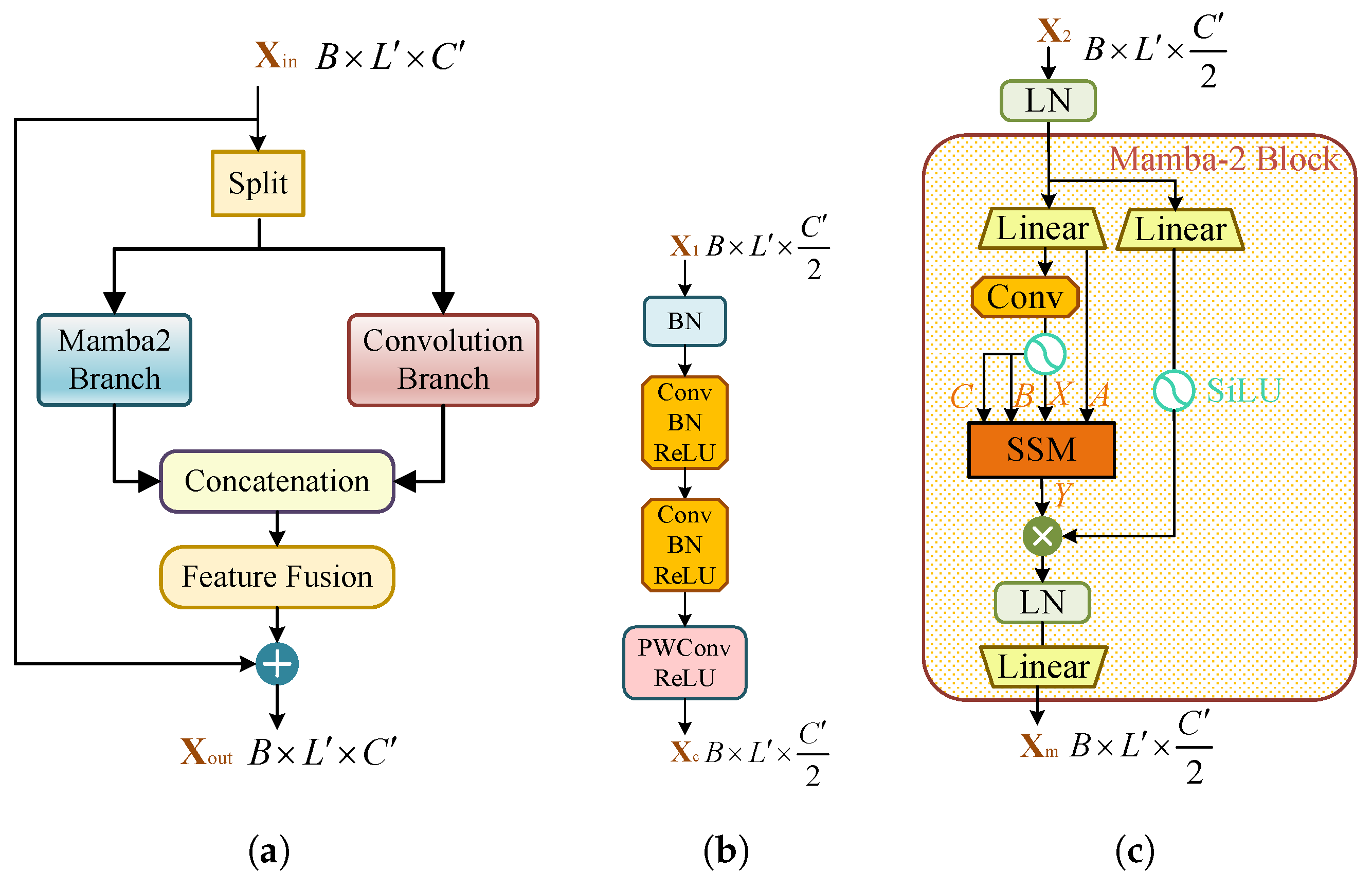
The core component of the ConvMamba model is the CNN–Mamba2 module, which has a dual-branch structure, as shown in Figure 5. Given an input feature ${\mathbf{X}}_{in}\in {\mathbb{R}}^{B\times L^{\prime }\times C^{\prime }}$, the module first splits the input feature along the channel dimension, evenly dividing it into two groups of features:

$${\mathbf{X}}_1,{\mathbf{X}}_2=\mathrm{split}\left({\mathbf{X}}_{in}\right)\in {\mathbb{R}}^{B\times L^{\prime }\times C^{\prime }/2},$$

(10)

where $\mathrm{split}(·)$ denotes division along the channel dimension. The two groups of features ${\mathbf{X}}_1$ and ${\mathbf{X}}_2$ then undergo different processing branches: the convolution branch captures local features, while the Mamba2 branch extracts global information. The overall structure of the CNN–Mamba2 module is shown in Figure 5a.

(1) For the convolution branch, the calculation process is shown in Figure 5b. This branch first rearranges the original feature map ${\mathbf{X}}_1$ to adjust its dimension order to adapt to the convolution operation:

$${\overline{\mathbf{X}}}_1\in {\mathbb{R}}^{B\times C^{\prime }/2\times L^{\prime }}\leftarrow \mathrm{permute}\left({\mathbf{X}}_1\right),$$

(11)

where $\mathrm{permute}(·)$ denotes dimension permutation. Then, feature processing is repeated through multiple convolutional (Conv) layers, batch normalization (BN) layers, and activation function (ReLU) layers. Among them, the first two convolutional (Conv) layers are ordinary convolutions with a kernel size of 3, and the last convolutional layer is a pointwise convolution (PWConv) with a kernel size of 1. Finally, the features are rearranged again to restore the dimension, obtaining the convolution branch feature ${\mathbf{X}}_c\in {\mathbb{R}}^{B\times C^{\prime }/2\times L^{\prime }}$.

(2) For the Mamba2 branch, the calculation process is shown in Figure 5c. This branch first performs layer normalization (LN) on ${\mathbf{X}}_2$, then extracts features through the Mamba2 block structure [27]. The Mamba2 block first performs linear mapping (Linear) and convolution (Conv) operations on the input to obtain the input (X) with structured state-space duality and parameter matrices A, B, and C, then calculates the output through a selective state-space model (SSM) with matrix operations. Meanwhile, residual connections (Linear+SiLu) are used to promote feature reuse. Finally, layer normalization (LN) is performed to enhance the stability of the model training process, and the feature dimension is restored through linear mapping (Linear) to obtain the Mamba2 branch output ${\mathbf{X}}_m\in {\mathbb{R}}^{B\times C^{\prime }/2\times L^{\prime }}$.

To integrate the outputs of the two branches, the module reconstructs the feature dimension through channel concatenation (Concatenate) and introduces a mixing mechanism (Shuffle) to fuse feature maps along the channel dimension:

$$\mathbf{Y}={\mathbf{X}}_{in}+\mathrm{shuffle}\left(\mathrm{concat}({\mathbf{X}}_c,{\mathbf{X}}_m)\right)$$

(12)

where $\mathbf{Y}$ is the output of the module, $\mathrm{shuffle}(·)$ denotes feature mixing along the channel dimension, and $\mathrm{concat}(·)$ denotes channel concatenation. The channel mixing design can effectively prevent information isolation between channels that may be caused by group computation.

In terms of activation function selection, the module inherits the choices of traditional CNN and Mamba2 architectures, using ReLU and SiLu activation functions in the two branches, respectively.

4. Experiments and Results Analysis

The effectiveness of the proposed ConvMamba model method was experimentally verified. In this section, the experimental settings (including dataset and model parameter settings) are first introduced; then, the experimental results are given, and the performance of the proposed ConvMamba model method is analyzed.

4.1. Experimental Settings

(1)

Dataset

To better evaluate the performance of the proposed model in processing complex high-order modulated signals, this study used the latest Sig53 dataset released by the U.S. Naval Research Laboratory [21] for evaluation. The dataset contains 5 million synthetic samples, covering rich high-order modulation types, and integrates various channel impairment models. In terms of modulation modes, the dataset includes 53 modulation types of different orders, involving mainstream modulation families such as ASK, PAM, PSK, QAM, FSK, and OFDM (as shown in

Table 1. Information of the Sig53 dataset [21].

Parameter	Details
Generation	Python3
Data format	I/Q, 2×4096
Sample size	Training: $5.3\times {10}^6$; Validation: $1.06\times {10}^5$
Modulation types	OOK, BPSK, 4PAM, 4ASK, QPSK, 8PAM, 8ASK, 8PSK, 16QAM, 16PAM, 16ASK, 16PSK, 32QAM, 32QAM_CROSS, 32PAM, 32ASK, 32PSK, 64QAM, 64PAM, 64ASK, 64PSK, 128QAM_CROSS, 256QAM, 512QAM_CROSS, 1024QAM, 2FSK, 2GFSK, 2MSK, 2GMSK, 4FSK, 4GFSK, 4MSK, 4GMSK, 8FSK, 8GFSK, 8MSK, 8GMSK, 16FSK, 16GFSK, 16MSK, 16GMSK, OFDM-64, OFDM-72, OFDM-128, OFDM-180, OFDM-256, OFDM-300, OFDM-512, OFDM-600, OFDM-900, OFDM-1024, OFDM-1200, OFDM-2048
Noise	Additive White Gaussian Noise (AWGN)

). In particular, the dataset includes a large number of high-order modulation types, including 256QAM, 512QAM, and 1024QAM. In addition, it includes OFDM modulated signals with different numbers of subcarriers. To simulate various non-ideal effects in real communication environments, the dataset incorporates multiple channel impairment factors, including channel noise and fading, random impulse shaping, phase offset, time offset, frequency offset, I/Q imbalance, and random resampling. For random impulse shaping, the transmitter is based on a static pulse shaping scheme, while the receiver processes the received data using overlaid randomized pulse shaping filters. This enables the simulation of mismatch between the shaping pulses at the transmitter and receiver. These impairment factors are probabilistically applied to the original signals, enabling the dataset to exhibit diversity. Clearly, given the diversity of the dataset, using it allows for a better evaluation of the generalization capability of the proposed model and also facilitates comparison with the existing research literature in the field [21]. For practical systems that may employ a smaller set of modulation types, the proposed model can be directly used or fine-tuned accordingly. Table 1 summarizes the basic information of this dataset, while

Table 2. Channel impairments included in the dataset.

Signal Impairments	Detailed Information	Probability
AWGN	SNR range: −2 dB to 30 dB	100%
Random Pulse Shaping	Constellation diagrams: RRC filter, $\alpha \sim U(0.1,0.6)$	100%
	GFSK/GMSK: $BT\sim U(0.1,0.5)$
	FSK/MSK: Low-pass filter with random passband
Phase Shift	Range: $(-\pi ,\pi )$	90%
Time Shift	Range: −32 to +32 I/Q samples	90%
Frequency Shift	Range: −16% to 16% of the sampling rate	70%
Rayleigh Fading	Constellation diagrams: RRC filter, $\alpha \sim U(0.1,0.6)$	50%
	GFSK/GMSK: $BT\sim U(0.1,0.5)$
	FSK/MSK: Low-pass filter with random passband
I/Q Imbalance	Amplitude imbalance: −3 dB to +3 dB	90%
	Phase imbalance: $-\pi /180$ to $\pi /180$
	DC offset: −0.1 to +0.1 dB
Random Resampling	Range: 0.75 to 1.5	50%

details the impairments included in the dataset.

(2)

Experimental Environment and Parameter Settings

To ensure the rationality and reproducibility of the experiments, the experimental environment and model hyperparameter settings are introduced in detail here. Due to the large size of the Sig53 dataset, 901,000 signals were randomly selected as training data in this experiment, with 90,100 samples in both the test set and validation set. The experiment used a server configured with an NVIDIA A6000 GPU (NVIDIA, Santa Clara, CA, USA) as the computing platform, the PyTorch 2.3.1 deep learning framework in the model implementation, and Python 3.10 for programming development in the PyCharm 2024 integrated development environment. The model optimizer used Adam, the learning rate was changed with the training process through a cosine annealing strategy, and the loss function used cross-entropy loss commonly used in multi-classification problems.

(3)

Benchmark Model Methods

To verify the effectiveness of the proposed ConvMamba model, two baseline methods were introduced in the experiment: EfficientNet based on the CNN architecture [21] and XCiT-Nano based on the Transformer architecture [21]. These two models are benchmark methods proposed in [21] for the Sig53 dataset. Among them, EfficientNet has three versions: EfficientNet-B0, EfficientNet-B2, and EfficientNet-B4 (abbreviated as EffNet-B0, EffNet-B2, and EffNet-B4). The differences between different versions mainly lie in the model parameter scale: EfficientNet-B0 is the smallest with 3.93 M parameters, and EfficientNet-B4 is the largest with 17.21 M parameters. As the model scale increases, the computational complexity and inference time of the model increase, and the recognition accuracy also increases. In addition, the MAWDN method proposed in [28] was also introduced for comparison and analysis.

To evaluate the impact of model scale on its performance, three versions of the ConvMamba model with different scales were designed in the experiment: ConvMamba-Tiny, ConvMamba-Small, and ConvMamba-Base (abbreviated as CM-T, CM-S, and CM-B). The main differences between these versions lie in the number of stacked CNN–Mamba2 modules and the number of channels in each stage. Different CNN–Mamba2 sizes represent different feature extraction capabilities and computational complexities: the CNNMamba2 module of CM-T is relatively small, so its computational complexity is low, but its feature extraction capability is relatively weak; the CNN–Mamba2 module of CM-B is the largest, so its computational complexity is higher, but its feature extraction capability is also stronger. Detailed architecture specifications are shown in

Table 3. Parameter settings for different model versions.

Layer Name	CM-T	CM-S	CM-B
Conv 1D	Number of channels → 64		Number of channels → 128
Denoising	Soft - threshold denoising
Stage-1	CNN–Mamba2 Block × 1	CNN–Mamba2 Block × 2	CNN–Mamba2 Block × 2
Path-M	Number of channels → 128		Number of channels → 256
Stage-2	CNN–Mamba2 Block × 1	CNN–Mamba2 Block × 2	CNN–Mamba2 Block × 2
Path-M	Number of channels → 256		Number of channels → 512
Stage-3	CNN–Mamba2 Block × 2	CNN–Mamba2 Block × 4	CNN–Mamba2 Block × 4
Path-M	Number of channels → 512		Number of channels → 768
Stage-4	CNN–Mamba2 Block × 1	CNN–Mamba2 Block × 2	CNN–Mamba2 Block × 2
Classifier	Global average pooling, linear layer, Softmax

.

It should be noted that to ensure the objectivity and comparability of the experimental results, all comparison methods in this study were re-implemented and tested in the same hardware and software environment rather than directly citing the results reported in the literature or using pre-trained model parameters. This method can eliminate performance deviations caused by differences in experimental platforms, ensuring the rationality and reliability of the comparison experiments.

4.2. Experimental Results and Analysis

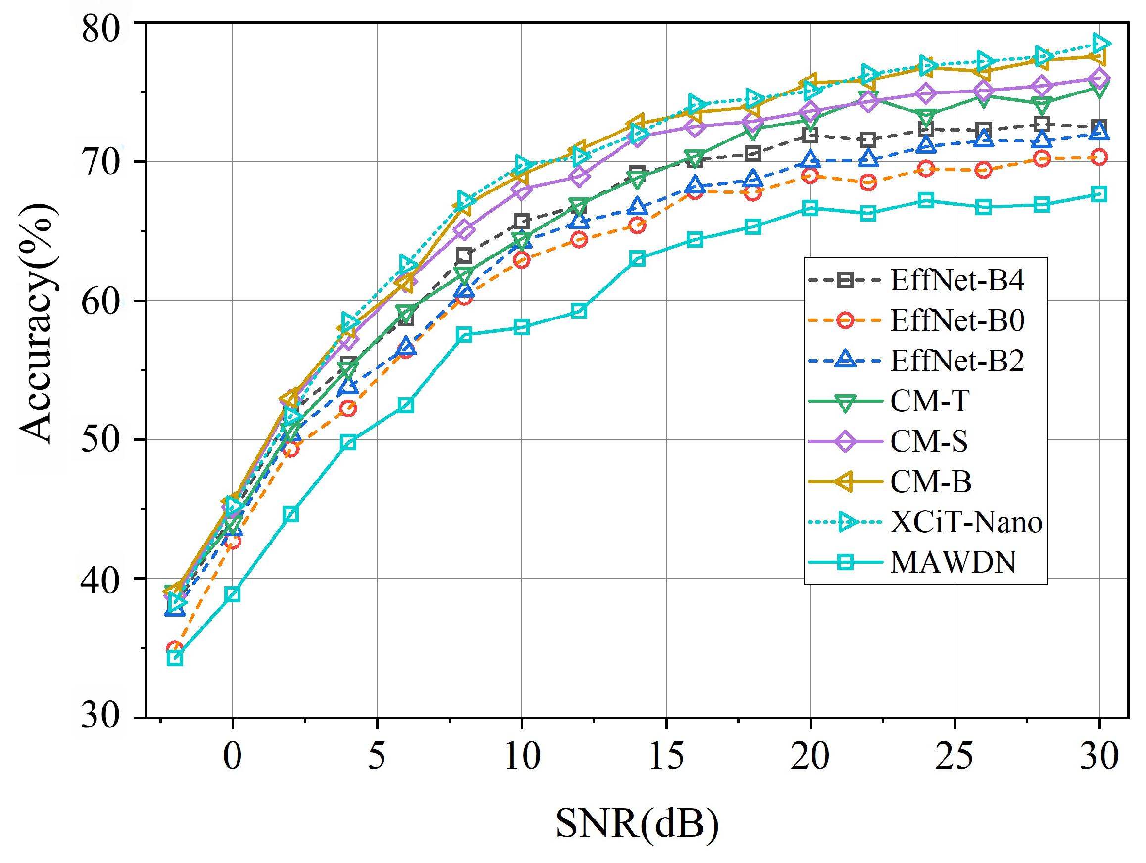
First, the recognition accuracy, computational complexity, inference time, and parameter quantity of each model are analyzed through experiments, and the results are shown in

Table 4. Performance of models based on different architectures.

Model	Parameters (M)	MACs (MMac)	Inference Time (s)	Accuracy (%)
EffNet-B0	3.93	537.04	0.023	61.3
EffNet-B2	7.56	989.88	0.027	62.1
EffNet-B4	17.21	2270	0.037	64.0
CM-T	2.04	841.6	0.025	64.9
CM-S	3.63	1460	0.043	66.1
CM-B	4.64	1980	0.086	67.1
XCiT-Nano	2.83	5130	0.186	67.3
MAWDN	0.60	345.61	0.047	58.3

(the batch size for testing inference time is 64). It can be seen from Table 4 that the smallest model CM-T proposed in this paper has higher accuracy than all versions of EfficientNet and has significant advantages in resource efficiency: the computational load of CM-T is only 1/3 of that of EffNet-B4, and the number of learnable parameters is only 1/5 of that. Compared with EffNet-B2 with comparable resource consumption, CM-T shows obvious advantages in accuracy. This result indicates that compared with CNN-based models, the proposed hybrid architecture model can more effectively capture and utilize long-range temporal dependency information, thereby achieving better recognition performance with lower resource consumption. Compared with the Transformer-based XCiT-Nano model, although XCiT-Nano has a slightly higher accuracy than CM-B, its computational demand is almost 2.6 times that of CM-B, which further verifies the superiority of the Mamba2-based ConvMamba architecture in balancing resource efficiency and recognition performance.

Figure 6 shows the trend of the recognition accuracy of each model with the change in signal-to-noise ratio (SNR). It can be seen that the recognition accuracy of all models increases with the increase in SNR, which is in line with expectations. In addition, among all comparison models, the largest-scale XCiT-Nano achieves the highest recognition accuracy, followed by the various versions of the proposed ConvMamba model, then the three versions of EfficientNet, and MAWDN has the worst performance, indicating that the lightweight designed MAWDN has insufficient ability to capture the features of high-order modulated long-sequence signals.

To further evaluate the performance advantages of the proposed model in high-order modulation type recognition,

Table 5. F1 scores of CM-T and EffNet-B4 on high-order modulation types.

Modulation Type	CM-T	EffNet-B4	Modulation Type	CM-T	EffNet-B4
64ASK	0.362	0.335	1024QAM	0.374	0.290
64PSK	0.369	0.346	OFDM-512	0.580	0.623
64PAM	0.572	0.492	OFDM-600	0.532	0.624
64QAM	0.375	0.326	OFDM-900	0.597	0.490
128QAM	0.299	0.257	OFDM-1024	0.551	0.506
256QAM	0.212	0.194	OFDM-1200	0.588	0.494
512QAM	0.335	0.300	OFDM-2048	0.648	0.587

shows the F1 score comparison between CM-T and the benchmark model EffNet-B4 on high-order modulation types. The F1 score, as the harmonic mean of precision and recall, can comprehensively reflect the comprehensive recognition ability of the model and is a key indicator for evaluating modulation recognition performance. For single-carrier high-order modulation types, the F1 scores of CM-T on QAM modulation types are all higher than those of EffNet-B4, indicating that the proposed model has excellent performance in processing complex modulated signals with densely distributed constellation points. At the same time, better performance on 64ASK and 64PAM (two high-order amplitude modulation types) indicates that the proposed model also has strong recognition ability in processing high-order amplitude and phase modulated signals. In terms of modulated signal recognition of OFDM series, CM-T achieves significant improvements in F1 scores for all other OFDM modulation types except for OFDM-512 and OFDM-600. Table 5 comprehensively shows that compared with the traditional CNN architecture, the proposed hybrid model fused with Mamba2 can more effectively capture discriminative features in high-order modulated signals, thereby achieving more accurate recognition.

Figure 7 presents the confusion matrix of the CM-T model, from which the differences in recognition difficulty of different modulation types can be observed. The derived or optimized frequency shift keying (FSK) modulated signals show high recognizability, mainly due to their unique frequency characteristics and strong antinoise ability. The distinction within OFDM categories is also relatively easy, with only slight confusion between high-order OFDM modulation types, which is mainly due to the multi-carrier and frequency domain distribution characteristics of OFDM signals, making them remain highly recognizable even under high-order modulation conditions. The most challenging tasks occur in amplitude and phase modulation types such as PAM/ASK/PSK/QAM. Figure 8 provides a more detailed visualization of these easily confusable modulation types. The results in Figure 8a indicate that confusion does not primarily occur between modulation types like PAM, ASK, PSK, and QAM. Instead, Figure 8b–e demonstrate that confusion mainly arises within the same modulation type across different modulation orders.

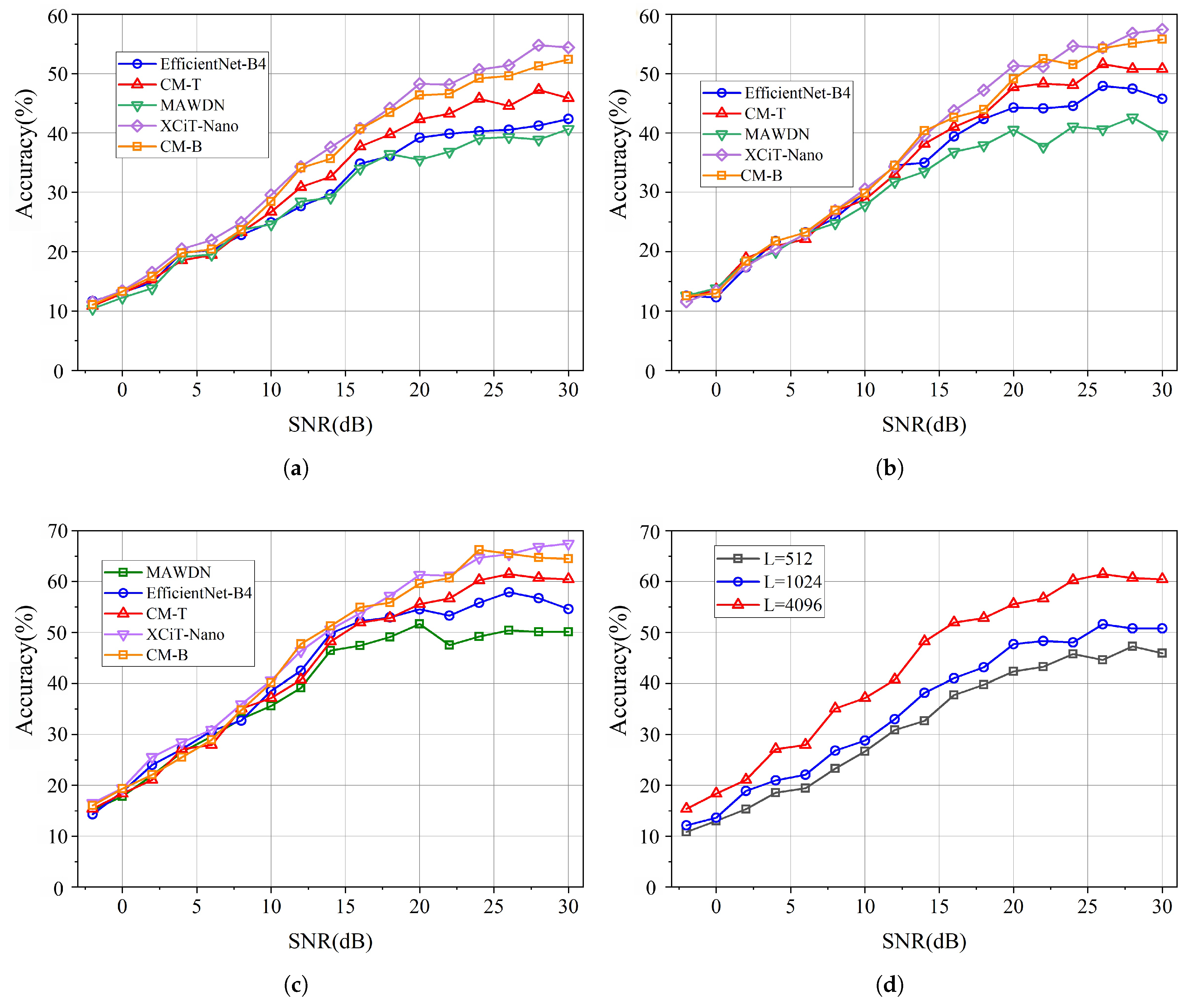
To evaluate the adaptability and performance of the proposed method in processing signals of different lengths, a comprehensive set of comparison experiments was designed here. The TorchSig [21] toolbox was used to generate test signals of different sampling lengths to verify the model’s adaptability to changes in signal length. To balance the computational resource requirements of the experiment and the comprehensiveness of the evaluation, four of the most challenging modulation families in the Sig53 dataset were selected based on the confusion matrix: PAM, ASK, PSK, and QAM (a total of 23 modulation modes) for testing. The training set had 391,000 samples, and the validation and test sets each had 39,100 samples; the signal lengths were set to 512, 1024, and 4096 sampling points, respectively. Other signal parameters and signal impairment settings were completely consistent with the Sig53 dataset shown in Table 1 and Table 2; the experimental results are shown in Figure 9 and

Table 6. Relation between F1 score and signal length for different modulation types.

Modulation Type	Sequence Length			Modulation Type	Sequence Length
	512	1024	4096		512	1024	4096
4PAM	0.659	0.682	0.788	32PAM	0.201	0.169	0.298
4ASK	0.555	0.635	0.707	32ASK	0.223	0.299	0.343
QPSK	0.595	0.607	0.686	32PSK	0.147	0.184	0.204
8PAM	0.424	0.467	0.599	64QAM	0.141	0.261	0.291
8ASK	0.414	0.356	0.506	64PAM	0.391	0.411	0.418
8PSK	0.352	0.402	0.460	64ASK	0.285	0.227	0.281
16QAM	0.300	0.410	0.485	64PSK	0.192	0.110	0.286
16PAM	0.287	0.309	0.447	128QAM_CROSS	0.151	0.173	0.243
16ASK	0.263	0.225	0.267	256QAM	0.184	0.144	0.156
16PSK	0.210	0.309	0.351	512QAM_CROSS	0.229	0.265	0.375
32QAM	0.230	0.382	0.489	1024QAM	0.250	0.284	0.326
32QAM_CROSS	0.342	0.409	0.465

.

Figure 9a–c demonstrate the performance of different methods with three signal length configurations. The results indicate that compared to the CNN-based EfficientNet architecture, the proposed ConvMamba model exhibits significant performance advantages across all signal length conditions. Simultaneously, the performance gap between ConvMamba and XciT-Nano progressively narrows as signal length increases, suggesting that ConvMamba can more effectively extract signal features from longer sequences. Figure 9d further compares the performance characteristics of the proposed CM-T model with different signal lengths. Additionally, the results confirm that recognition accuracy increases with longer signal lengths, aligning with expectations since higher-order modulation signals require longer sample sequences to capture richer signal features for improved identification accuracy.

Table 6 presents the F1 score variations of the CM-T model for different modulation types across signal lengths. The results demonstrate a significant upward trend in F1 scores for most modulation types as signal sampling length increases. This confirms a positive correlation between signal sequence length and modulation recognition performance. For higher-order modulation types, this performance improvement is particularly pronounced. For instance, the F1 score for 64QAM more than doubles when the length increases from 512 to 4096 samples. This indicates that extending the observation window enables the model to capture richer modulation features, thereby enhancing discriminative capability for higher-order modulations.

A noteworthy observation can be discerned from Figure 6: during the recognition process for the Sig53 dataset, even under the high signal-to-noise ratio condition of SNR = 30 dB, the recognition accuracy still fails to exceed 90%. This result indicates that in higher-order modulation signal recognition tasks, signal-to-noise ratio is no longer the sole dominant factor affecting recognition performance. To further investigate this, we conducted an in-depth exploration into the impact of different channel impairments on DL-AMR recognition performance, particularly focusing on the most challenging signal types in the Sig53 dataset: PAM, ASK, PSK, and QAM. Using the TorchSig toolbox under the high SNR = 30 dB condition, different types of channel impairments, namely, no impairment, phase shift, time offset, frequency shift, I/Q imbalance, resampling, and Rayleigh fading, were individually applied to PAM, ASK, PSK, and QAM signals, and the results are shown in Figure 10. Specifically, the parameters for each impairment were kept consistent with those in Table 2, with the difference being that instead of applying impairments to the signals with a certain probability, each of the aforementioned impairments was applied separately to all test signals. That is, each impairment acted on the signal independently, in order to evaluate the individual impact of each type of impairment. As can be seen from the figure, I/Q imbalance has minimal impact on recognition accuracy. Frequency offset, phase noise, timing offset, and resampling cause moderate performance degradation, while Rayleigh fading has the most severe impact on recognition performance, leading to a significant reduction in accuracy. This result indicates that channel fading constitutes one of the most challenging factors in the recognition process for long-sequence modulation signals.

5. Conclusions

This paper studies high-order modulated signal recognition and proposes a ConvMamba model method that integrates CNN and Mamba2 hybrid architectures. It effectively captures temporal dependency features in long-sequence signals through a selective state-space model and combines the local feature extraction capability of convolutional neural networks to form a hybrid network structure with both global modeling and local feature extraction advantages. In addition, the model enhances anti-noise performance using a designed soft-threshold denoising module. Experimental verification on the Sig53 dataset and TorchSig toolbox shows that compared with traditional models based on CNN and Transformer architectures, ConvMamba achieves a better balance between computational efficiency and recognition accuracy. In addition, as can be seen from the experimental results, the proposed method still achieves very low recognition accuracy with low signal-to-noise ratios and certain specific modulation modes, that is, an Accuracy below 60% and an F1 score of less than 0.2. This indicates that the proposed model is completely impractical. Therefore, it remains necessary to explore more robust model approaches in the future. Possible strategies include introducing complex-valued neural networks or adopting hierarchical classification recognition strategies, among others.

References

1. Huynh-The, T.; Pham, Q.V.; Nguyen, T.V.; Nguyen, T.T.; Ruby, R.; Zeng, M.; Kim, D.S. Automatic Modulation Classification: A Deep Architecture Survey. IEEE Access 2021, 9, 142950–142971. [Google Scholar] [CrossRef]
2. Xie, W.; Hu, S.; Yu, C.; Zhu, P.; Peng, X.; Ouyang, J. Deep Learning in Digital Modulation Recognition Using High Order Cumulants. IEEE Access 2019, 7, 63760–63766. [Google Scholar] [CrossRef]
3. Wang, X.; Zhao, Y.R.; Huang, Z.T. A Survey of Deep Transfer Learning in Automatic Modulation Classification. IEEE Trans. Cogn. Commun. Netw. 2025, 11, 1357–1381. [Google Scholar] [CrossRef]
4. Peng, S.; Sun, S.; Yao, Y.D. A Survey of Modulation Classification Using Deep Learning: Signal Representation and Data Preprocessing. IEEE Trans. Neural Netw. Learn. Syst. 2021, 33, 7020–7038. [Google Scholar] [CrossRef] [PubMed]
5. O’Shea, T.J.; Corgan, J.; Clancy, T.C. Convolutional Radio Modulation Recognition Networks. In Proceedings of the 17th International Conference on Engineering Applications of Neural Networks (EANN), Aberdeen, UK, 2–5 September 2016; pp. 213–226. [Google Scholar]
6. Rajendran, S.; Meert, W.; Giustiniano, D.; Lenders, V.; Pollin, S. Deep Learning Models for Wireless Signal Classification with Distributed Low-Cost Spectrum Sensors. IEEE Trans. Cogn. Commun. Netw. 2018, 4, 433–445. [Google Scholar] [CrossRef]
7. Dai, A.; Zhang, H.J.; Sun, H. Automatic Modulation Classification Using Stacked Sparse Auto-Encoders. In Proceedings of the 2016 IEEE 13th International Conference on Signal Processing (ICSP), Chengdu, China, 6–10 November 2016; pp. 248–252. [Google Scholar]
8. Vaswani, A.; Shazeer, N.; Parmar, N.; Uszkoreit, J.; Jones, L.; Gomez, A.N.; Kaiser, Ł.; Polosukhin, I. Attention Is All You Need. Adv. Neural Inf. Process. Syst. 2017, 30, 6000–6010. [Google Scholar]
9. West, N.E.; Shea, T.O. Deep Architectures for Modulation Recognition. In Proceedings of the 2017 IEEE International Symposium on Dynamic Spectrum Access Networks (DySPAN), Baltimore, MD, USA, 6–9 March 2017; pp. 1–6. [Google Scholar]
10. Xu, J.; Luo, C.; Parr, G.; Luo, Y. A Spatiotemporal Multi-Channel Learning Framework for Automatic Modulation Recognition. IEEE Wirel. Commun. Lett. 2020, 9, 1629–1632. [Google Scholar] [CrossRef]
11. Njoku, J.N.; Morocho-Cayamcela, M.E.; Lim, W. CGDNet: Efficient Hybrid Deep Learning Model for Robust Automatic Modulation Recognition. IEEE Netw. Lett. 2021, 3, 47–51. [Google Scholar] [CrossRef]
12. Ma, J.T.; Qiu, T.S. Automatic Modulation Classification Using Cyclic Correntropy Spectrum in Impulsive Noise. IEEE Wirel. Commun. Lett. 2019, 8, 440–443. [Google Scholar] [CrossRef]
13. Li, Y.B.; Shao, G.P.; Wang, B. Automatic Modulation Classification Based on Bispectrum and CNN. In Proceedings of the 2019 IEEE 8th Joint International Information Technology and Artificial Intelligence Conference (ITAIC), Chongqing, China, 24–26 May 2019; pp. 311–316. [Google Scholar]
14. Teng, C.F.; Liao, C.C.; Chen, C.H.; Wu, A.Y.A. Polar Feature Based Deep Architectures for Automatic Modulation Classification Considering Channel Fading. In Proceedings of the 2018 IEEE Global Conference on Signal and Information Processing (GlobalSIP), Anaheim, CA, USA, 26–28 November 2018; pp. 554–558. [Google Scholar]
15. Kosuge, D.; Otsuka, H. Transmission Performance of OFDM-based 1024-QAM under Different Types of Multipath Fading Channels. In Proceedings of the 2021 IEEE VTS 17th Asia Pacific Wireless Communications Symposium (APWCS), Osaka, Japan, 30–31 August 2021. [Google Scholar]
16. Khorov, E.; Levitsky, I.; Akyildiz, I.F. Current Status and Directions of IEEE 802.11be, the Future Wi-Fi 7. IEEE Access 2020, 8, 88664–88688. [Google Scholar] [CrossRef]
17. Bauwelinck, J.; De Backer, E.; Melange, C.; Torfs, G.; Ossieur, P.; Qiu, X.-Z. A 1024-QAM Analog Front-End for Broadband Powerline Communication Up to 60 MHz. IEEE J. Solid-State Circuits 2009, 44, 1234–1245. [Google Scholar] [CrossRef]
18. Xu, Y.Q.; Xu, G.X.; Ma, C. A Novel Blind High-Order Modulation Classifier Using Accumulated Constellation Temporal Convolution for OSTBC-OFDM Systems. IEEE Trans. Circuits Syst. II 2022, 69, 3959–3963. [Google Scholar] [CrossRef]
19. Zhang, Y.; Zhou, Z.; Cao, Y.; Li, G.; Li, X. MAMC—Optimal on Accuracy and Efficiency for Automatic Modulation Classification With Extended Signal Length. IEEE Commun. Lett. 2024, 28, 2864–2868. [Google Scholar] [CrossRef]
20. He, J.; Xu, C.; Yin, C.; Zhang, Y. High-Order Modulation Recognition of Communication Signals Based on Feature Fusion. In Proceedings of the 2024 IEEE 7th Information Technology, Networking, Electronic and Automation Control Conference (ITNEC), Chongqing, China, 20–22 September 2024. [Google Scholar]
21. Boegner, L.; Gulati, M.; Vanhoy, G.; Vallance, P.; Comar, B.; Kokalj-Filipovic, S.; Lennon, C.; Miller, R.D. Large Scale Radio Frequency Signal Classification. arXiv 2022, arXiv:2207.09918. [Google Scholar] [CrossRef]
22. Cai, J.J.; Gan, F.M.; Cao, X.H.; Liu, W. Signal Modulation Classification Based on the Transformer Network. IEEE Trans. Cogn. Commun. Netw. 2022, 8, 1348–1357. [Google Scholar] [CrossRef]
23. Ma, W.X.; Cai, Z.R.; Wang, C. A Transformer and Convolution-Based Learning Framework for Automatic Modulation Classification. IEEE Commun. Lett. 2024, 28, 1392–1396. [Google Scholar] [CrossRef]
24. Gu, A.; Dao, T. Mamba: Linear-Time Sequence Modeling With Selective State Spaces. arXiv 2023, arXiv:2312.00752. [Google Scholar] [CrossRef]
25. Liu, M.; Guo, F.; Chen, Y.; Zhao, N. Blind Modulation Classification for OFDM in the Presence of Carrier Frequency Offsets. In Proceedings of the 2023 IEEE International Conference on Communications (ICC), Rome, Italy, 28 May–1 June 2023. [Google Scholar]
26. Zhao, M.; Zhong, S.; Fu, X.; Tang, B.; Pecht, M. Deep Residual Shrinkage Networks for Fault Diagnosis. IEEE Trans. Ind. Inform. 2020, 16, 4681–4690. [Google Scholar] [CrossRef]
27. Dao, T.; Gu, A. Transformers Are SSMs: Generalized Models and Efficient Algorithms Through Structured State Space Duality. arXiv 2024, arXiv:2405.21060. [Google Scholar] [CrossRef]
28. Qin, X.; Jiang, W.; Gui, G.; Li, D.; Niyato, D.; Lu, J. Multilevel Adaptive Wavelet Decomposition Network Based Automatic Modulation Recognition: Exploiting Time-Frequency Multiscale Correlations. IEEE Trans. Cogn. Commun. Netw. 2025; early access. [Google Scholar]
Figure 1. B asic workflow of DL-AMR.
Applsci 15 09805 g001
Figure 2. Overall structure of CNN–Mamba2.
Applsci 15 09805 g002
Figure 3. Structure of the soft-threshold denoising module.
Applsci 15 09805 g003
Figure 4. Computation process of the feature fusion module.
Applsci 15 09805 g004
Figure 5. Structure of the CNN–Mamba2 module. (a) Overall structure of CNN–Mamba2. (b) Convolutional branch. (c) Mamba2 branch.
Applsci 15 09805 g005
Figure 6. Accuracy variation of the proposed method and baseline models with different SNRs.
Applsci 15 09805 g006
Figure 7. Confusion matrix of CM-T.
Applsci 15 09805 g007
Figure 8. Confusion of CM-T on different modulation types. (a) Inter-class confusion matrix. (b) Intra-class PAM confusion matrix. (c) Intra-class ASK confusion matrix. (d) Intra-class QAM confusion matrix. (e) Intra-class PSK confusion matrix.
Applsci 15 09805 g008
Figure 9. Performance of the proposed method on signals with different lengths. (a) Signal length = 512 samples. (b) Signal length = 1024 samples. (c) Signal length = 4096 samples. (d) Performance of CM-T model with different signal lengths.
Applsci 15 09805 g009
Figure 10. Impact of different channel impairments on DL-AMR performance.
Applsci 15 09805 g010