Fine-Tuning a Large Language Model for the Classification of Diseases Caused by Environmental Pollution

Abstract

Environmental pollution poses an increasing threat to public health, particularly in urban areas with high levels of pollutant exposure. To address this challenge, this study proposes a model based on fine-tuning the LLaMA 3 large language model for the classification of pollution-related diseases using user-reported symptoms. A balanced dataset was employed, with examples evenly distributed across 10 common diseases, and several preprocessing techniques were applied, including tokenization, normalization, noise removal, and data augmentation. The model was fine-tuned using the QLoRA technique, which integrates quantization with low-rank adaptation, enabling both training and inference on resource-constrained hardware. During training, a consistent reduction in loss and a progressive improvement in validation accuracy were observed. Moreover, the confusion matrix demonstrated a high classification success rate with minimal misclassification across classes. The findings suggest that optimized large language models can be effectively applied in settings with limited computational infrastructure, supporting the early diagnosis of diseases associated with environmental factors.

1. Introduction

1.1. Impact of Pollution on Health

Environmental pollution represents a growing threat to global public health. According to the World Health Organization (WHO), exposure to air pollutants such as fine particulate matter (PM_2.5), nitrogen dioxide (NO₂), ozone (O₃), and other toxic gases significantly contributes to premature mortality in millions of individuals. Urban and industrial regions, where pollutant concentrations are highest, face particularly severe challenges in maintaining air quality and mitigating its effects on vulnerable populations, including children, the elderly, and individuals with pre-existing chronic conditions [1]. Chronic exposure to these pollutants has been linked to a broad spectrum of diseases, the most common of which are chronic respiratory diseases, including chronic bronchitis, chronic obstructive pulmonary disease (COPD), asthma, sinusitis, and other pulmonary conditions that impair respiratory function. Additionally, pollution can also cause dermatological conditions and other systemic pathologies due to exposure to environmental toxic agents [1].

1.2. Challenges for Early Diagnosis

Early detection of these diseases is essential to prevent their progression and reduce their impact on patients’ quality of life. However, the variability of symptoms and their overlap with those of other conditions complicate accurate diagnosis, particularly in healthcare settings with limited resources or restricted access to specialists. Consequently, the development and implementation of technological tools to support early diagnosis have become an urgent necessity, especially in regions heavily affected by environmental pollution [2].

1.3. Advances in Large Language Models

Large Language Models (LLMs) have emerged as a revolutionary advancement in natural language processing (NLP), distinguished by their ability to handle vast amounts of textual data. These models have demonstrated outstanding performance, enabling advancements in areas that include automatic medical data analysis [3,4]. Nevertheless, despite their great potential, current LLMs face important limitations due to high computational requirements and the lack of adaptation to specific contexts, including diseases associated with environmental pollution [5,6]. The use of LLMs in the medical field in Spanish-speaking countries is still an underexplored area, especially in contexts such as environmental pollution, where colloquial language plays a crucial role. In Spanish-speaking countries, the use of LLMs in the medical domain remains underexplored, particularly in contexts related to environmental pollution, where colloquial language plays a pivotal role. In Mexico, for example, regional variations in Spanish, informal expressions, and frequent spelling errors hinder the effectiveness of pre-existing models, limiting their applicability in real-world scenarios. Models such as LLaMA 3, when fine-tuned with approaches like QLoRA, offer the potential to address these challenges and enhance the classification of symptoms in high environmental impact contexts [7].

1.4. Challenges in Medical Text Classification

Medical text classification, particularly in contexts with high linguistic variability such as Spanish spoken in Mexico, presents a significant challenge for pre-existing language models. Although models like BERT have demonstrated strong performance in general text classification tasks [7,8,9,10], their effectiveness diminishes when addressing tasks involving regional variations or frequent spelling errors [7]. Fine-tuning advanced models, such as LLaMA 3, with techniques like QLoRA, provide an effective solution by adapting the models to these linguistic conditions, thereby improving accuracy in the classification of diseases associated with environmental pollution [7].

Despite recent advances in the application of LLMs in the medical field, significant limitations persist, particularly related to high computational costs and the need for specialized infrastructure [11,12]. These barriers restrict access to such models, especially in resource-limited regions. To address this issue, optimization techniques such as LoRA and QLoRA have been developed, enabling the deployment of models in environments with more modest computational capacity [13,14]. In particular, QLoRA, by combining quantization with low-rank adaptation, provides an efficient alternative that substantially reduces memory and computational demands without compromising performance [14].

The classification of medical tests using large language models (LLMs) has proven effective in identifying symptoms and diseases from written clinical information, thereby enhancing the capacity of systems to interpret complex medical records [15]. Additionally, research on diseases associated with environmental pollution has demonstrated how exposure to allergens and pollutants influences both the onset and severity of respiratory conditions, including asthma and other allergic disorders [16]. These findings underscore the importance of developing models capable of analyzing clinical text while accounting for variations in symptom presentation, particularly in contexts where environmental factors exert a substantial impact on health.

1.5. Research Objectives

This study aims to adapt and fine-tune the LLaMA 3 language model using the QLoRA technique to optimize its ability to classify diseases associated with environmental pollution. The model is designed as a supportive tool for symptom interpretation, intended to guide the identification of potential conditions without substituting professional medical diagnosis. Furthermore, the study proposes a performance comparison between the base model and the fine-tuned version. A key challenge addressed is the reduction in computational requirements, thereby enabling the model’s deployment in resource-limited settings, such as rural clinics or regions with limited technological infrastructure.

Furthermore, the creation of a balanced dataset representing a wide range of pollution-related diseases is proposed. This dataset will undergo medical validation to ensure that all included examples are clinically relevant and representative of the conditions to be classified. By incorporating diversity and balance, the dataset will enable the model to generalize effectively while minimizing bias toward majority classes. An important contribution of this work is the integration of diverse linguistic features, particularly from regions such as central Mexico, where specific language variations are common. This linguistic richness will allow the model to classify symptoms with greater accuracy and contextual relevance in areas heavily affected by pollution.

2. Materials and Methods

Figure 1 presents the general workflow of the research process, which is structured into five main stages. The first stage involves dataset construction, including data collection, dataset assembly, data augmentation, noise removal, normalization, balancing, labeling, and validation in Spanish, followed by the generation of embedding vectors for processing. In the second stage, a Transformer-based large language model is selected; in this case study, the LLaMA 3 model with 8 billion parameters is chosen as the base model. The third stage consists of fine-tuning using the QLoRA technique, in which quantization is applied to reduce the size of the model’s weights and overall footprint, while LoRA matrices are incorporated during the training process. This results in the development of a new model trained on a dataset of symptoms associated with environmental pollution. Finally, the model’s performance is validated in the subsequent stages using a range of evaluation metrics to assess its effectiveness in text classification tasks.

2.1. Construction and Processing of the Dataset

The dataset employed in this study contains symptomatic information related to 10 diseases associated with environmental pollution. These diseases were selected based on their high incidence in areas with elevated levels of air pollution and were categorized into four groups—respiratory, cardiovascular, dermatological, and other conditions linked to polluted environments:

• Laryngitis;
• Bronchiectasis;
• Ischemic heart disease;
• Chronic bronchitis;
• Pulmonary emphysema;
• Sinusitis;
• Respiratory allergy;
• COPD (Chronic Obstructive Pulmonary Disease);
• Interstitial lung disease;
• Vasomotor rhinitis.

The dataset is composed of two primary elements:

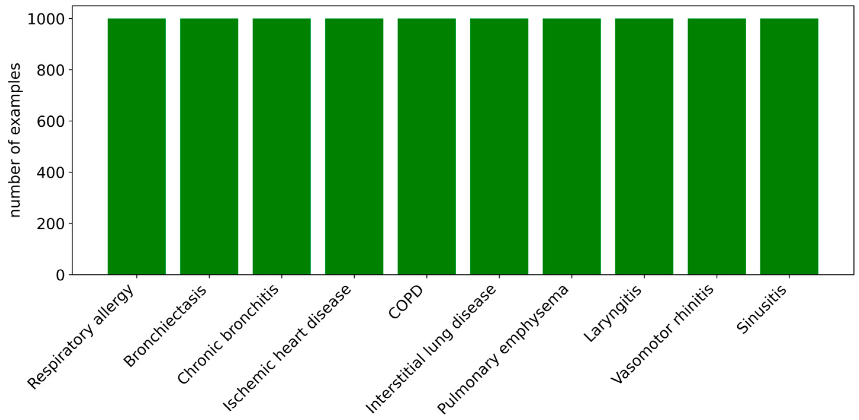
• Disease label: Each record in the dataset is associated with a label corresponding to a specific disease. Each category is represented by 1000 examples, resulting in a total of 10,000 examples in Spanish. Importantly, the dataset is balanced, ensuring that the model can make predictions without bias toward any particular class.
• Data augmentation: To enhance the robustness of the dataset, several augmentation techniques were applied, including the use of synonyms, translations, misspellings, and common slang expressions.

Reported symptoms: Each entry in the dataset includes a description of the symptoms reported by individuals. This information was obtained from self-reports of people exposed to pollution, complemented with documented data on the typical symptoms of associated diseases. All entries were subsequently validated by healthcare professionals to ensure clinical relevance and accuracy.

The use of the Spanish language in this study is based on the need to address health problems derived from environmental pollution in Mexico, specifically in the central region of the country, where exposure to air pollutants such as nano-particles affects a large part of the population, especially in urban and industrial areas. In this context, cities such as Mexico City, Puebla, Hidalgo, and Toluca are particularly vulnerable due to high concentration of pollutants. The model developed in this work is based on data from approximately 150 people, whose symptoms were described in both formal and informal language characteristics of this region, allowing for better understanding and classification of diseases caused by pollution.

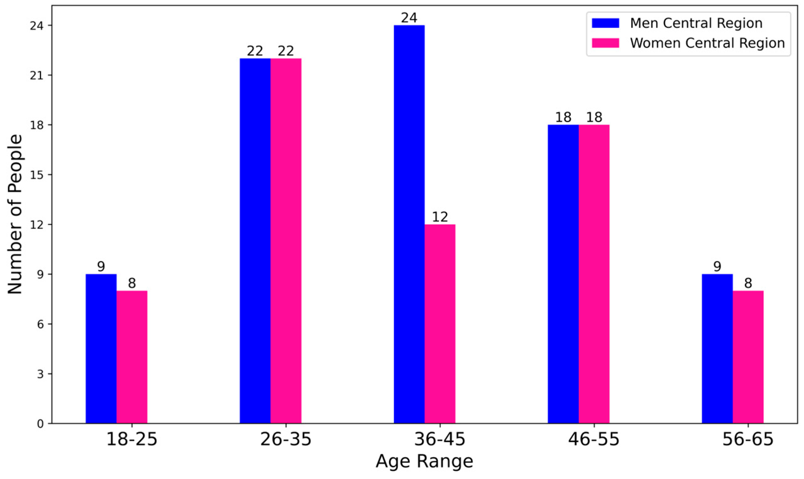
The sample of 150 people is composed of a balanced distribution by gender and age, as shown in Figure 2. Approximately 55% of the participants are men, and 45% are women. As for the age range, participants are between 18 and 65 years old, including both young adults and middle-aged individuals, who are more susceptible to the effects of prolonged exposure to pollution. Most of the participants come from areas in central Mexico, more specifically from Mexico City, Ciudad Sahagún (Hidalgo), and Pachuca (Hidalgo), which are regions with high levels of air pollution, particularly due to vehicular traffic, industrial activities, and waste burning.

The data were collected through structured forms and mobile applications, all distributed online. These instruments included both closed and open-ended questions, allowing participants to freely describe their symptoms and any potential pollution-related health conditions. Participants provided their information voluntarily, and anonymity as well as confidentiality were strictly maintained. The information gathered included recently experienced symptoms, their duration, and exposure to pollution sources such as vehicular traffic, industrial facilities, or waste burning.

To enhance monitoring and obtain more detailed information, a mobile application was employed to enable participants to record their symptoms in real time on a daily basis. Through this application, users could provide continuous information on the progression of their symptoms, which contributed to building a more representative dataset of daily health fluctuations. This data collection methodology—online surveys and mobile applications—ensured that the symptom descriptions reflected participants’ everyday experiences, including informal and colloquial expressions common in the region, such as “Hoy amanesi todo fregado” or “Ora si q amanci re mal”. Incorporating such expressions is essential for training diagnostic models capable of handling region-specific colloquial language.

Before being used for training, the data underwent a preprocessing pipeline designed to adapt it to the model requirements. This process comprised the following phases:

• Normalization. The text is adjusted to ensure consistency by removing unnecessary special characters, standardizing the use of uppercase and lowercase letters, and applying lemmatization (reducing words to their root form). This procedure reduces model complexity and enhances generalization.
• Noise removal. Irrelevant or repetitive elements that could interfere with model learning—such as excessive punctuation and stopwords (e.g., the, of, and)—were removed.
• Class balance verification. The dataset was evaluated to ensure that the classes were sufficiently balanced, thereby preventing bias toward categories with a larger number of examples.
• Tokenization and embedding. The symptom reports were segmented into smaller units, such as words or subwords. Subsequently, each token was transformed into a high-dimensional numerical vector through embedding. These dense vector representations capture both semantic meaning and contextual relationships, enabling the model to interpret the underlying patterns in the reported symptoms.

At this point, the Transformer architecture is employed. It not only processes with these numerical representations but also assigns them contextual meaning and a position within the sequence—without the need for recurrent mechanisms, such as those used in recurrent neural networks (RNNs). Instead of processing words one by one, the Transformer uses self-attention to analyze the relationships among all the words in the sequence simultaneously [17].

For a neural network to process text, it is necessary to transform those words into a numerical representation, since networks cannot directly understand human language. This transformation is performed through tokenization and embedding generation, where tokens (words or subwords) are converted into numerical vectors that encode their semantic and contextual information.

Below is a function that converts words into numerical vectors with a fixed size.

$$f:V\to R^d,$$

(1)

where V is the vocabulary (with |V| distinct words) and d is the dimension of the embedding vector space, typically between 300 and 512 dimensions for Transformer models.

The embedding is used by the model to represent words (or tokens) in a high-dimensional vector space. These dimensions of the embedding are crucial because they affect the model’s ability to capture semantic and syntactic relationships between words in the text.

A larger embedding dimension allows the model to capture more complex and detailed word representations. This is especially important when the model works with large data volumes. If the embedding dimension is insufficiently large, the model may fail to capture important semantic nuances. Conversely, if it is excessively large, the model may represent unnecessarily complex patterns, leading to higher computational costs and an increased risk of overfitting.

The function f assigns to each word w_i a vector $v_i\in {\mathbb{R}}^d$, and these vectors are stored in an embedding vector matrix. Therefore, when the neural network is provided with a sequence of words (tokens), it converts this sequence into a sequence of dense vector representations.

$$E=\left[v_1,v_2,v_3\dots v_n\right].$$

(2)

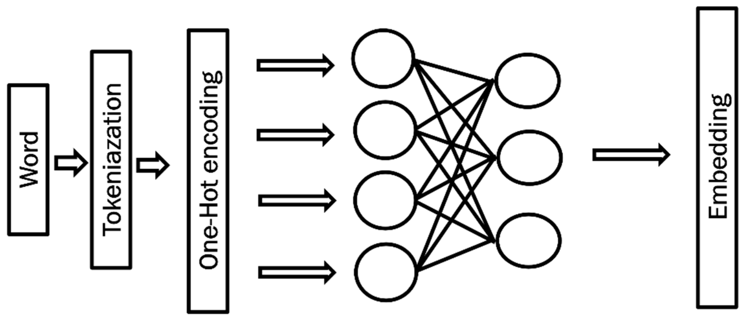
Figure 3 illustrates the process of obtaining an embedding vector from a word. First, the input word undergoes tokenization, which converts it into a token, i.e., a basic unit such as a word, subword, or symbol. This token is then represented using one-hot encoding, producing a binary vector of length equal to the vocabulary size, with a single active element set to 1 and all others set to 0, thereby indicating the identity of the word.

This one-hot vector is subsequently fed into a neural network—typically an embedding layer or a dense layer—that transforms the sparse, high-dimensional representation into a dense, lower-dimensional vector. During training, the neural network learns to assign weights so that the resulting vectors capture semantic and contextual relationships between words. In this way, the model produces an embedding vector: a continuous numerical representation that reflects both the meaning of the word and its relationships within the vector space.

The Transformer does not process text sequentially; instead, it processes all elements in parallel. A limitation of this approach is that the positional order of the tokens within the sequence is not inherently encoded. Therefore, positional information must be incorporated to indicate the order of the words.

This information is represented by a vector that is added to the embedded vector of each token to include details about its position in the sequence.

$${PE}_{(pos,2i)}=sin\left({\displaystyle \frac{pos}{{10000}^{2i/d}}}\right),$$

(3)

$${PE}_{(pos,2i+1)}=cos\left({\displaystyle \frac{pos}{{10000}^{2i/d}}}\right).$$

(4)

A unique representation is assigned to each position in a sequence. The variable pos indicates the position of a token within the sequence, while $i$ is an index referring to a particular dimension of the encoding. d is the total dimension of the encoding, controlling the size of the vector space. The encoding is performed using sine and cosine functions, calculating ${PE}_{(pos,2i)}$ with the sine function and ${PE}_{(pos,2i+ 1)}$ with the cosine function. The scaling factor $\mathrm{10,000}$ adjusts the frequencies of these functions, allowing the capture of spatial relationships at different scales within the sequence [18,19].

It contains a representation of both the embedding vector information and the positional information.

$$x_t=v_t+p_t,$$

(5)

where $x_t$ is the new vector including the embedded vector and the positional information of the token, $v_t$ is the embedding vector, and $p_t$ is the vector of positional information.

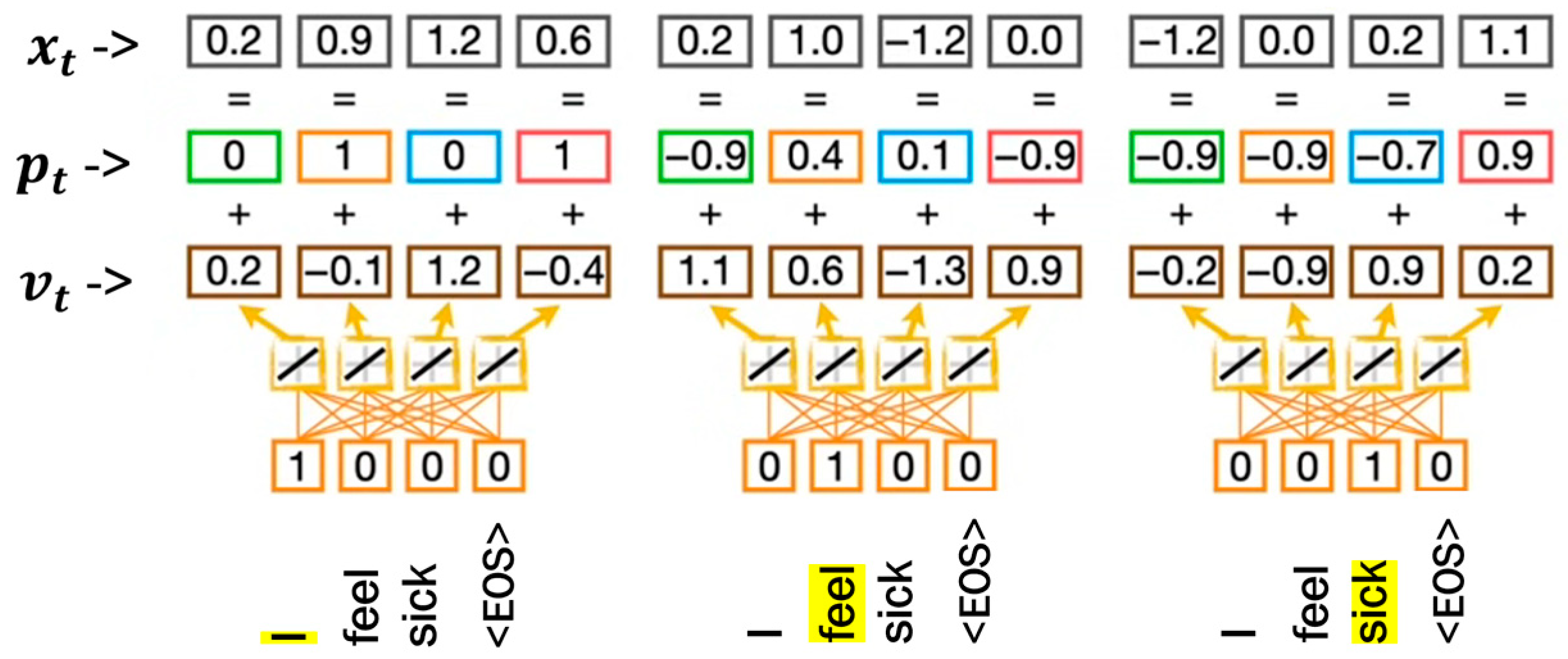
Figure 4 illustrates the process through which a word is tokenized and initially represented as a one-hot vector, denoted as $v_t$, which is the output of the neural network and contains the dense representation or embedding of the token. To each embedding vector, a positional encoding vector $p_t$ is added, which encodes the token’s location within the sequence to preserve order and context. The element-wise sum of $v_t$ and $p_t$ yields the vector $x_t$, which is the final representation that combines both the semantic information of the token and its position in the sequence.

In general, the self-attention mechanism evaluates all words within a sentence, assigning relevance scores to each token to capture the overall semantic meaning of the sentence. This enables the model to effectively model the contextual dependencies among tokens in the sequence [17].

$$K=x{W}_k,$$

(6)

$$V=x{W}_v,$$

(7)

$$Q=x{W}_q,$$

(8)

where the calculation of the Q (query), K (key), and V (value) vectors is carried out in the self-attention mechanism of Transformer models. In each case, the input x (which can be a token or an intermediate representation of the sequence) is multiplied by a specific weight matrix Q, K, or V. The Q vector represents the query, K the key for determining the relevance of positions in the sequence, and V contains the information that is passed as output, weighted by the attention calculated from the relationship between Q and K. These vectors are fundamental for the attention calculation, where queries are compared with keys to obtain weights that are applied to the values, thus producing the output of the attention mechanism [20,21,22].

$$Attention\left(Q,K,V\right)=softmax\left({\displaystyle \frac{Q{K}^T}{\sqrt{d_k}}}\right)V,$$

(9)

where Q, K, and V are the vectors calculated earlier, d_k is the dimension of the vectors, and softmax is a function that normalizes the values. The operation QK^T calculates the similarity between the queries and the keys, and the result is scaled by dividing by the square root of the dimension d_k to avoid excessively large values. Then, the softmax function is applied to obtain attention weights, which are used to weigh the values V. The result is the output of the attention layer, a weighted representation of the values based on their relevance in the sequence.

2.2. Base Model

LLaMA 3 is a large language model based on the Transformer architecture, representing the third generation of the LLaMA family developed by Meta AI. This model is distinguished by its capacity to process and generate text with high accuracy, enabled by an architecture that leverages the multi-head attention mechanism to capture complex contextual relationships across long textual sequences.

The Transformer architecture employed in LLaMA 3 is composed of stacked layers of self-attention and feed-forward networks. Each layer includes a multi-head autoregressive self-attention module, which allows the model to assign relative importance weights to tokens with respect to others within the sequence, as well as a feed-forward neural network that processes this information to capture higher-level patterns. Multi-head attention enhances the model’s ability to attend to different parts of the text simultaneously, thereby improving its understanding of global context and long-range dependencies [17].

In the version used for this study, LLaMA 3 has approximately 8 billion parameters distributed across 32 layers. Each layer has a model dimension of 4096 and an internal feed-forward network (FFN) dimension of 14,336. The network uses 32 attention heads, organized into 8 groups for key and value operations. The activation function employed is SwiGLU, which combines linearity with nonlinear activation, enhancing the model’s capacity to represent complex relationships in text [7]. Meanwhile, the larger versions, with 70 billion and 405 billion parameters, have more complex configurations due to their size, as shown in

Table 1. Features of LLaMA 3 model.

Features	8B	70B	405B
FFN Dimension	14,336	28,672	53,548
Key/Value Heads	8	8	8
Layers	32	80	126
Model Dimension	4096	8192	16,384
Attention Heads	32	64	128
Vocabulary Size	128,000
Positional Embeddings	RoPE (θ = 500,000)

.

The model’s vocabulary contains 128,000 tokens, enabling efficient and detailed handling of natural language across multiple languages. LLaMA 3 is a multilingual model trained on large-scale datasets in diverse languages, which provides it with the capability to both understand and generate text in various linguistic contexts. For this study, the primary focus is on the Spanish language, since the symptomatic descriptions and clinical data come from native speakers or users expressing themselves in this language. This ensures accurate comprehension and reliable classification of environmental diseases described in Spanish.

By and large, these technical features provide LLaMA 3 with a robust capacity to model the semantic and syntactic structures of clinical texts and symptoms expressed in natural language, which makes it particularly well-suited for text-based classification and diagnosis tasks in Spanish and other languages.

QLoRA is a technique that optimizes the fine-tuning of language models by reducing memory usage through quantization and low-rank matrices. This approach enables pre-trained models to be fine-tuned on hardware with limited resources, decreasing both computational load and storage requirements. As a result, it achieves satisfactory performance without the extensive resource demands typical of other fine-tuning methods [14].

2.3. Quantization

Quantization is a technique that reduces the numerical precision of a model’s parameters by converting 32-bit floating-point values into lower-bit representations (e.g., 8-bit integers). This process decreases model size and improves computational efficiency, particularly during training and inference. In this method, the base model’s weights are first normalized prior to quantization [14]:

$$x\prime ={\displaystyle \frac{x-\mu }{\sigma }},$$

(10)

where x′ is the normalized value, x is the original weight value, μ is the mean of the data, and is σ the standard deviation.

As its name suggests quantization is based on the process of converting continuous values into discrete ones. In the case of NF4, a 4-bit number (2⁴ = 16 possible levels) is used to represent each normalized value.

First, the normalized value x′ is mapped to one of the 16 values that can be represented in 4 bits.

$$q(x\prime )=round(x\prime ·(N-1\left)\right),$$

(11)

where q(x′) being the quantized value, while N = 16 is the number of possible levels in 4 bits, and the round function rounds to the nearest value.

Once the weights are quantized, it is necessary to reconstruct their values to the original floating-point domain. This is achieved with an inverse scaling to convert it back to its original range.

$$x″={\displaystyle \frac{q(x\prime )\left(\sigma \right)}{N-1}}+\mu .$$

(12)

2.4. LoRA

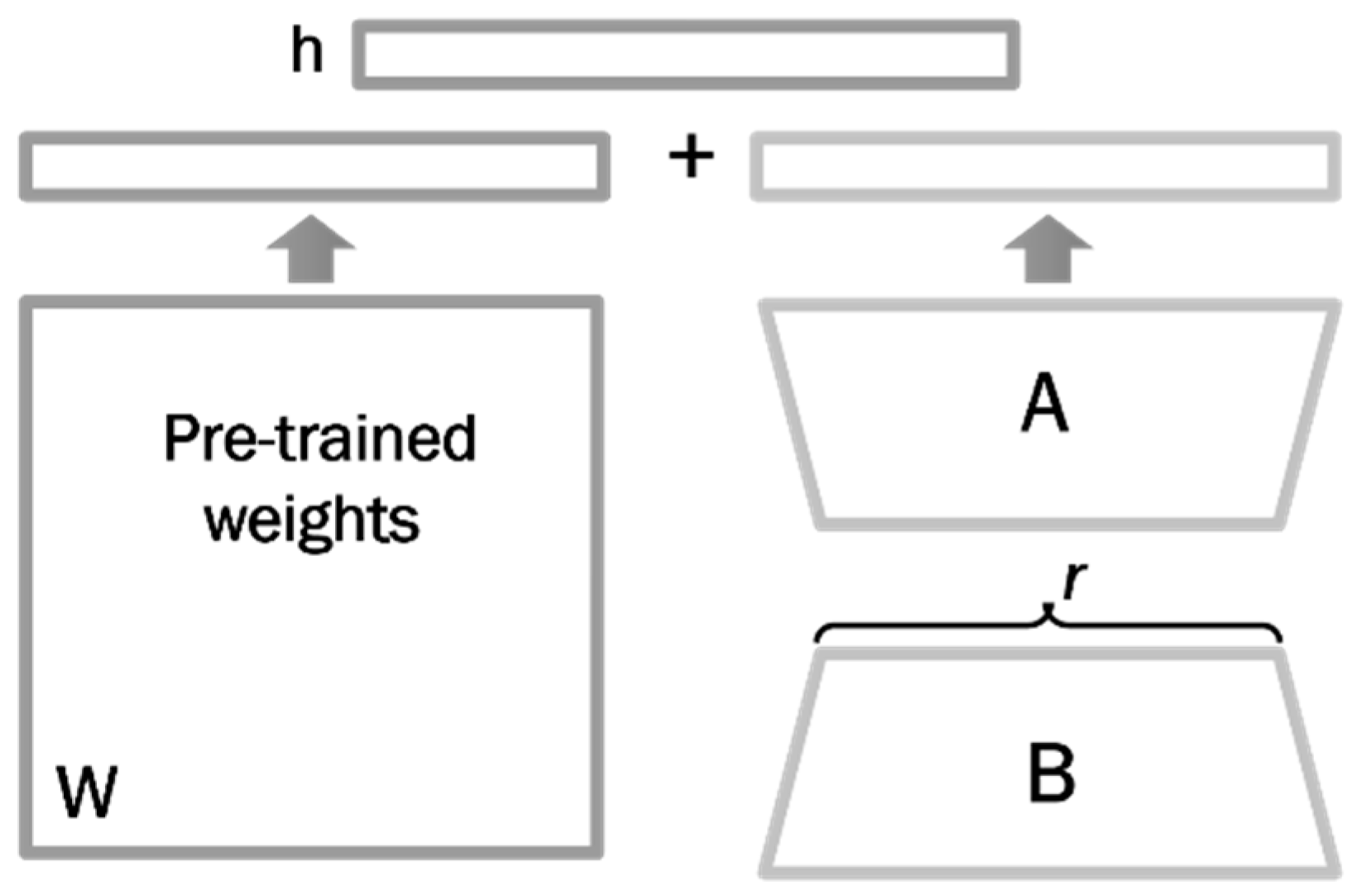
LoRA is a technique designed to adapt pre-trained models to specific tasks without requiring full retraining of all model parameters. In traditional models, weight matrices are typically large and high-rank, meaning that they consist of numerous parameters to be optimized. In contrast, LoRA introduces low-rank matrices with significantly fewer parameters, which are used to adapt specific components of the model while leaving most parameters unchanged.

The weight matrix of the base model remains frozen, and what is trained are the low-rank matrices A and B.

$$\mathrm{W}\prime =W+A B,$$

(13)

where W represents the original weights of the base model, while A and B are the low-rank matrices of size r × d and d × r, respectively. r being a low-rank hyperparameter and must be smaller than d (the size of the original matrix), as shown in Figure 5.

During the hyperparameter selection process, multiple experiments were conducted to adjust these values. The tests involved evaluating the model under different configurations and assessing convergence stability and predictive accuracy. Ultimately, the selected hyperparameters were those that offered good performance without overloading the system’s resources, rendering the model suitable for deployment in resource-constrained environments.

Table 2. Hyperparameters.

Hyperparameter	Value	Description
Learning_rate	1 × 10−4	Learning rate for the optimizer
per_device_train_batch_size	8	Batch size per device during training
LoRA rank (r)	16	Rank for the LoRA adaptation
LoRA alpha	8	Rank for the LoRA adaptation
per_device_eval_batch_size	8	Batch size per device during evaluation
LoRA_dropout	0.05	Dropout forregularization within LoRA
Max_LEN	512	Maximum token length for input truncation

shows that a learning rate value of 1 × 10⁻⁴ was chosen, which is a commonly used value in fine-tuning tasks for large models like LLaMA 3. This value was selected after conducting some preliminary tests that showed a higher learning rate caused oscillations in the loss function, while a lower rate resulted in slower training.

A batch size of 8 was selected for both training and evaluation. This value was chosen based on the memory limitations of the available hardware (GPU) and the need to maintain good performance. Although larger batch size could have accelerated training, tests were conducted showing memory issues arose with larger batches, which affected the stability of the training process.

The maximum sequence length was set to 512, which determines the maximum length of the texts that the model could process. Texts exceeding this length would be truncated. This value was chosen to ensure that the model could handle long sequences without compromising performance, as the model would be trained with texts of varying lengths.

As for the implementation, Python 3.12.9 was used as the main programming language due to its widespread adoption in the artificial intelligence community and its ecosystem of specialized libraries. The LLaMA 3 model and the fine-tuning process are based on PyTorch 2.5.1, given that it enables optimized tensor operations, thus facilitating execution on accelerated computing devices such as GPUs.

The training process incorporates the following key components:

• Central Processing Unit (CPU): Intel Core i5 12th Gen;
• Graphics Processing Unit (GPU): NVIDIA GeForce RTX 4060 Ti;
• Operating System: Windows 10 Pro.

The hyperparameters used during training are summarized as follows:

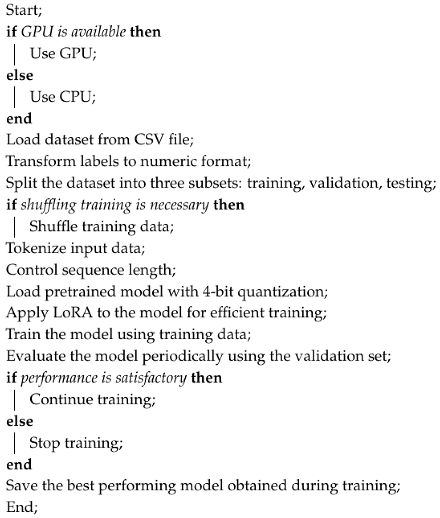
The process described below corresponds to the general structure of the code used to train and evaluate the model, as represented in Algorithm 1.

First, the code loads the dataset in CSV format, which contains the information necessary for training and evaluating the model. This step is essential to obtain the raw material to work with.

The data are subjected to a preprocessing pipeline that includes encoding the labels into a numerical format compatible with the model and splitting the original dataset into three disjoint subsets: training, validation, and test. This division enables the model to be trained, optimize its parameters, and subsequently be evaluated on unseen data, thereby ensuring robust generalization performance. The training set is then shuffled to mitigate potential biases from the original data ordering, improving both diversity and learning quality. Subsequently, the texts are transformed into numerical representations through tokenization, an essential step that enables the model to process textual information. At this stage, sequence length is also constrained to maintain computational efficiency.

Algorithm 1: Fine tuning pseudocode

Next, a pretrained model configured with 4-bit quantization is loaded, reducing memory requirements and resource usage during training, and thereby enabling large models to be executed on resource-constrained hardware. To further improve efficiency, the LoRA technique is applied, which modifies only a subset of the model parameters during fine-tuning, thereby enhancing training efficiency with respect to both memory and computational speed.

The model is trained using the prepared dataset and, during this process, its performance is periodically evaluated with the validation set to monitor progress and prevent overfitting. Based on these evaluations, the code decides whether to continue or stop training to ensure the model is optimally adjusted.

Finally, the best version of the model obtained during training is automatically saved, guaranteeing that the most efficient and accurate model is available for later use.

3. Results

3.1. Dataset

For data collection, a mixed approach was followed, combining bibliographic research with direct clinical information gathering. An initial review was performed to identify the ten most prevalent diseases associated with environmental pollution. Based on this research, the characteristic symptoms of each disease were selected, which served as the foundation for defining classification categories and designing the data collection protocol.

Subsequently, this information was complemented with data collected through structured interviews with patients diagnosed with one of the previously identified diseases. In addition, digital questionnaires and mobile applications were employed to monitor the daily progression of symptoms and patients’ overall health status, thereby capturing the variability and temporal dynamics of their symptoms throughout the day.

Regarding the number of participants, approximately 150 people were interviewed, ensuring diversity in terms of age, gender, and levels of environmental exposure. Each patient provided multiple records over time, resulting in a dataset of 4000 entries, reflecting the symptoms and disease progression in various contexts and at different times.

Once the data were obtained, the labeling protocol was designed, based on criteria defined from medical literature and clinical guidelines on diseases associated with environmental pollution. A labeling manual was created, which includes detailed instructions on which symptoms or combinations of symptoms correspond to each disease, along with examples and special cases to ensure that the labeling process was consistent and free from ambiguities. This protocol was essential to ensure that the labeling was consistent and reproducible, significantly reducing the subjectivity of the process.

To carry out the labeling, two professionals with medical training were selected. These professionals were responsible for reviewing and validating the recorded symptomatology of each disease and reviewing examples to unify criteria and ensure proper interpretation of the data.

To improve the representativeness of the dataset and increase the number of examples available for training the model, data augmentation techniques were implemented. Given that the original dataset consisted of a limited number of records, several strategies were employed to generate new examples without the need to collect more real data. The techniques employed were:

• Controlled paraphrasing. New instances were generated by synonymously rewording the symptom descriptions, maintaining their original meaning while varying both structure and vocabulary. This procedure introduced variations in the same symptom set without altering its clinical essence.
• Variation in description length. Entries were modified by altering their length, either by adding supplementary details or by simplifying existing content, thereby capturing greater diversity in the expression of symptoms.
• Introduction of controlled typographical errors. Typographical and spelling errors were intentionally introduced to simulate human data-entry behavior. This strategy enhanced the model’s robustness by teaching it to handle common errors likely to appear in real-world data.
• Translation and back-translation. A translation strategy was employed in which texts were translated into other languages and subsequently back into the original language, thereby introducing additional variability in symptom descriptions while preserving key information.

Once the data augmentation was completed, quality validation of the labels was carried out. The dataset was shuffled with a reproducibility index, and a representative sample of 10% of the dataset was selected to evaluate inter-labeler concordance. The inter-rater reliability was assessed using Cohen’s kappa coefficient, which quantifies the level of agreement between experts while correcting for chance agreement. The obtained value was κ = 0.85, indicating high concordance and, therefore, good confidence in the quality of the labeling.

The result is a dataset made of 10,000 balanced records, with validated symptomatology and labels for 10 diseases related to environmental pollution.

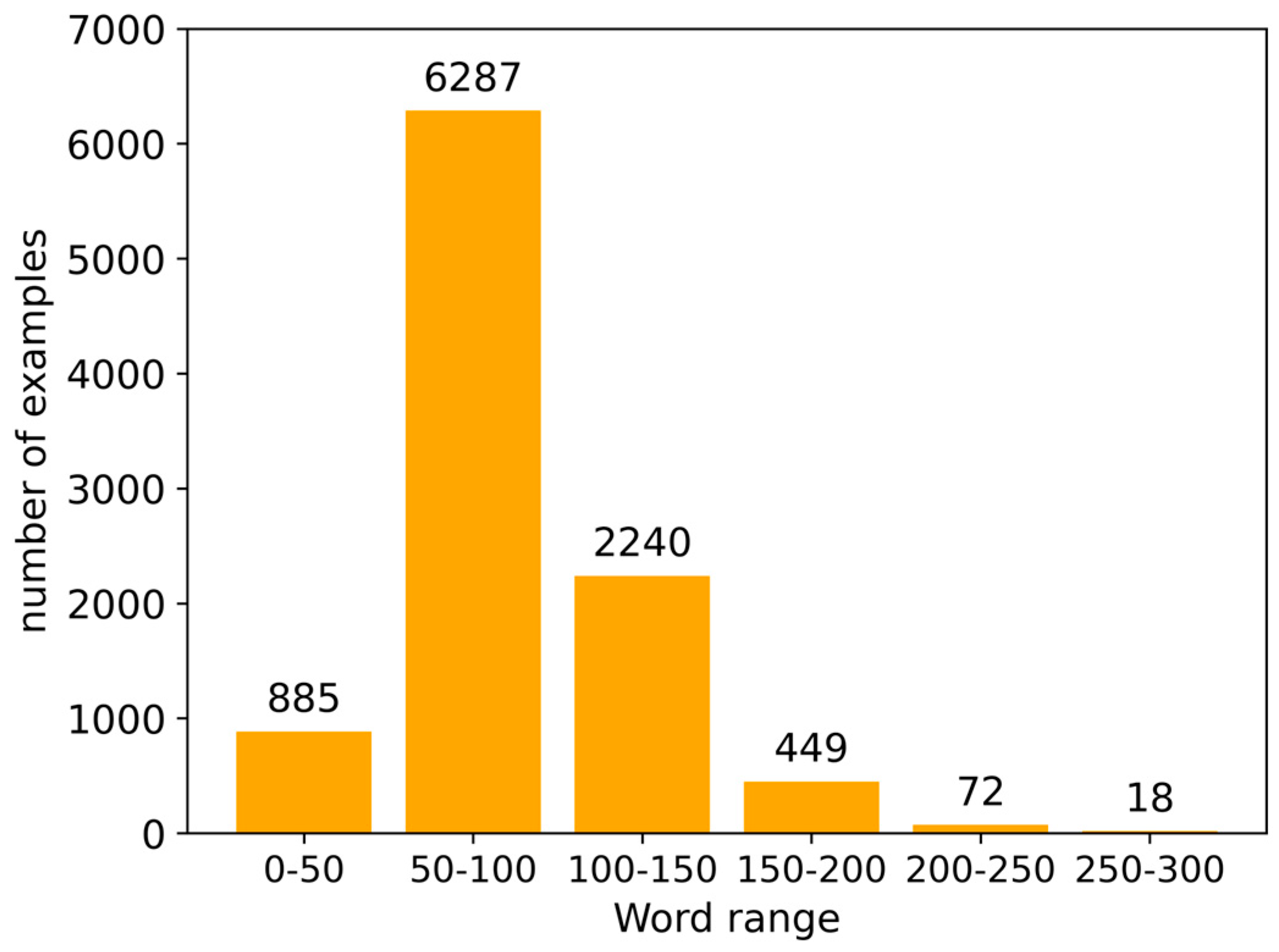
The number of examples in the dataset for different word ranges is shown in Figure 6. The bar corresponding to the 50–100 token range is the highest, comprising 6287 instances, which indicates that the majority of participants described their symptoms within this text length interval. This suggests that this range is the most suitable for describing symptoms in detail, but without being too short or too long. Since it is expected that new data will follow a similar pattern, with descriptions mostly within this range, the model can be optimized to efficiently handle texts between 50 and 100 words. While longer texts (e.g., those with 200 words or more) are less frequent, the model should also be prepared to manage those cases, although the primary focus should be on examples from the most common range.

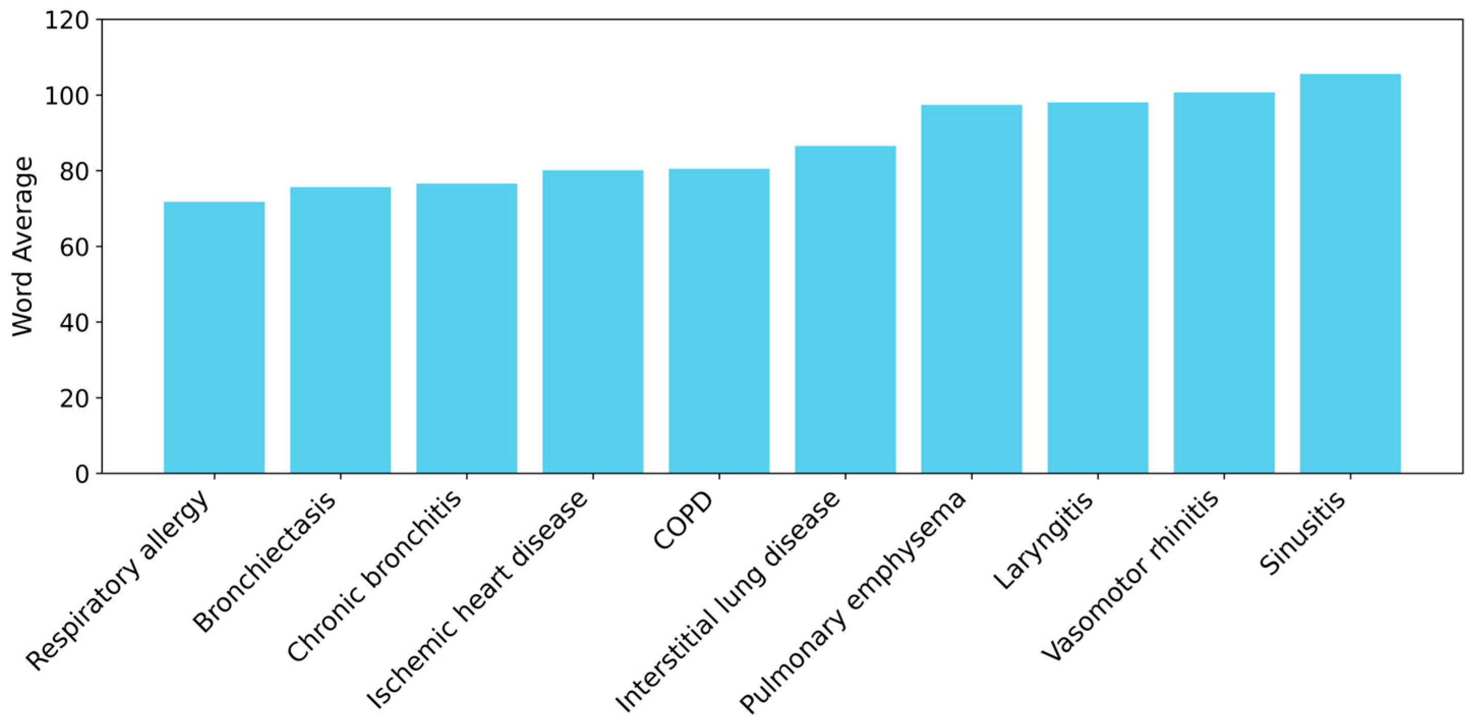
The adjusted average word count for each class is presented, predominantly representing respiratory diseases. The results indicate that, although some classes exhibit slightly higher average word counts, the differences across classes are not statistically significant. This suggests that the dataset is balanced with respect to description length per class. The minimal variation in length implies that the model will not need to handle substantial differences in text complexity across classes, as shown in Figure 7. Such balance is advantageous, as it enables more consistent and unbiased training without favoring classes with longer or more complex descriptions.

The number of examples available per class is presented in Figure 8, showing a balanced distribution with a similar number of instances across categories. This balance is advantageous, as it helps mitigate bias toward overrepresented classes during training. In the context of fine-tuning, it is essential to ensure that all classes are equally represented in the learning process, thereby preventing the model from favoring classes with more data, which could otherwise compromise its accuracy.

3.2. Text Processing

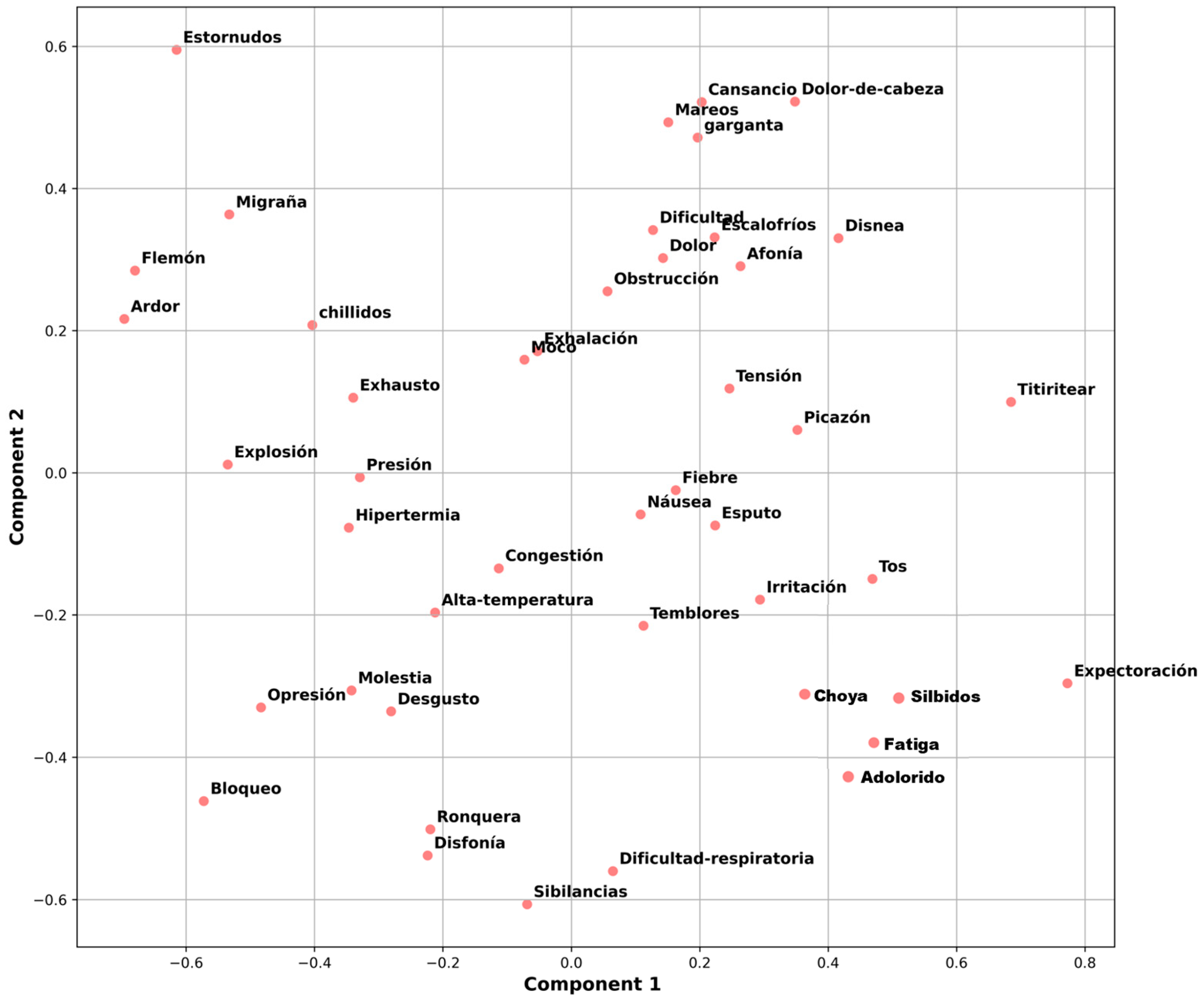
Figure 9 shows a two-dimensional graphical representation of the embedding vectors derived from the symptomatic dataset. These vectors correspond to the projection of key words and terms related to symptoms of environmental diseases into a high-dimensional vector space.

The observed clustering and dispersion reflect semantic relationships between words, where terms with similar meanings or contexts are positioned close to each other in space. For example, respiratory-related symptoms such as “Fiebre” and “Temblores” appear near one another, while others like “Dificultad-respiratoria” and “silbancias” form their own semantic cluster.

It is noteworthy that, despite the dataset containing misspelled words, abbreviations, and orthographic variations, the embedding process successfully maps these variants to proximate vectors, preserving their underlying meaning. This enables the model to correctly interpret these terms during training and prediction.

3.3. Training

The dataset was divided into three subsets:

• Test set (20%): This subset contains instances not included during training, providing an unbiased assessment of the model’s final performance. Since the model has not been exposed to these data beforehand, it cannot adjust its parameters to them, thereby enabling the evaluation of its generalization capability and its effectiveness on unseen or real-world data that may be encountered in future applications.
• Validation set (20%): This subset was employed to evaluate the model’s performance throughout training and to guide the adjustment of hyperparameters, including learning rate and batch size. As a dataset distinct from the training set, it enabled assessment of the model on unseen data, thereby preventing overfitting and promoting effective generalization.
• Training set (60%): This subset was employed to train the language model and optimize its parameters. It comprises the majority of the examples and enables the model to learn the relationships between symptoms and their associated diseases. By exposing the model to a wide variety of instances, the training set allows the model to learn patterns and correlations within the data, thereby supporting accurate predictions and relevant responses when applied to new or unseen cases.

3.3.1. Evolution of the Loss During Training

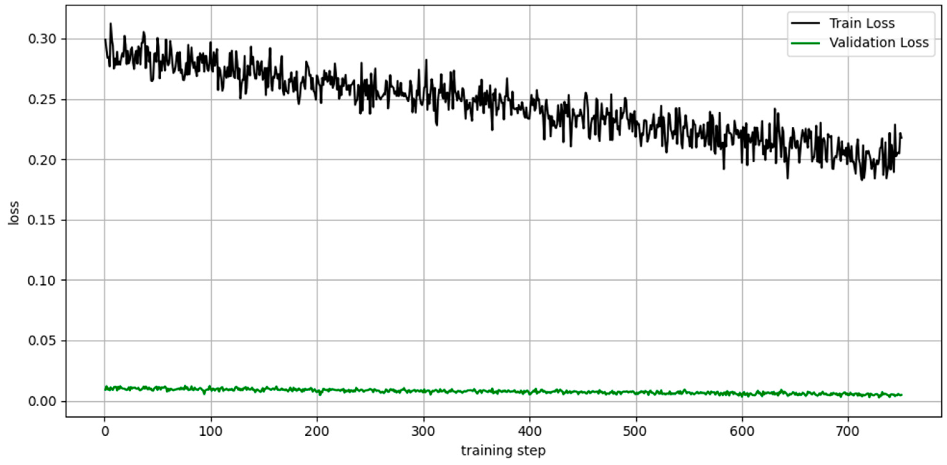
The graph shows the evolution of the loss during the training process. It displays the loss on the training set represented in black and the loss on the validation set represented in green, as shown in Figure 10. The Y-axis shows the loss, while the X-axis displays the number of training steps.

During training, the loss on the training set progressively decreases, indicating that the model is learning and adjusting its parameters correctly. On the other hand, the loss of the validation set follows a similar trend, albeit with a more gradual decrease. This suggests that the model is generalizing well, meaning it is learning to make accurate predictions on unseen data, although the validation loss may stabilize faster than the training loss, which is expected behavior.

The concurrent decrease in both losses over time indicates effective model training, with no apparent signs of overfitting, as the training and validation losses remain closely aligned.

3.3.2. Evolution of Accuracy During Training

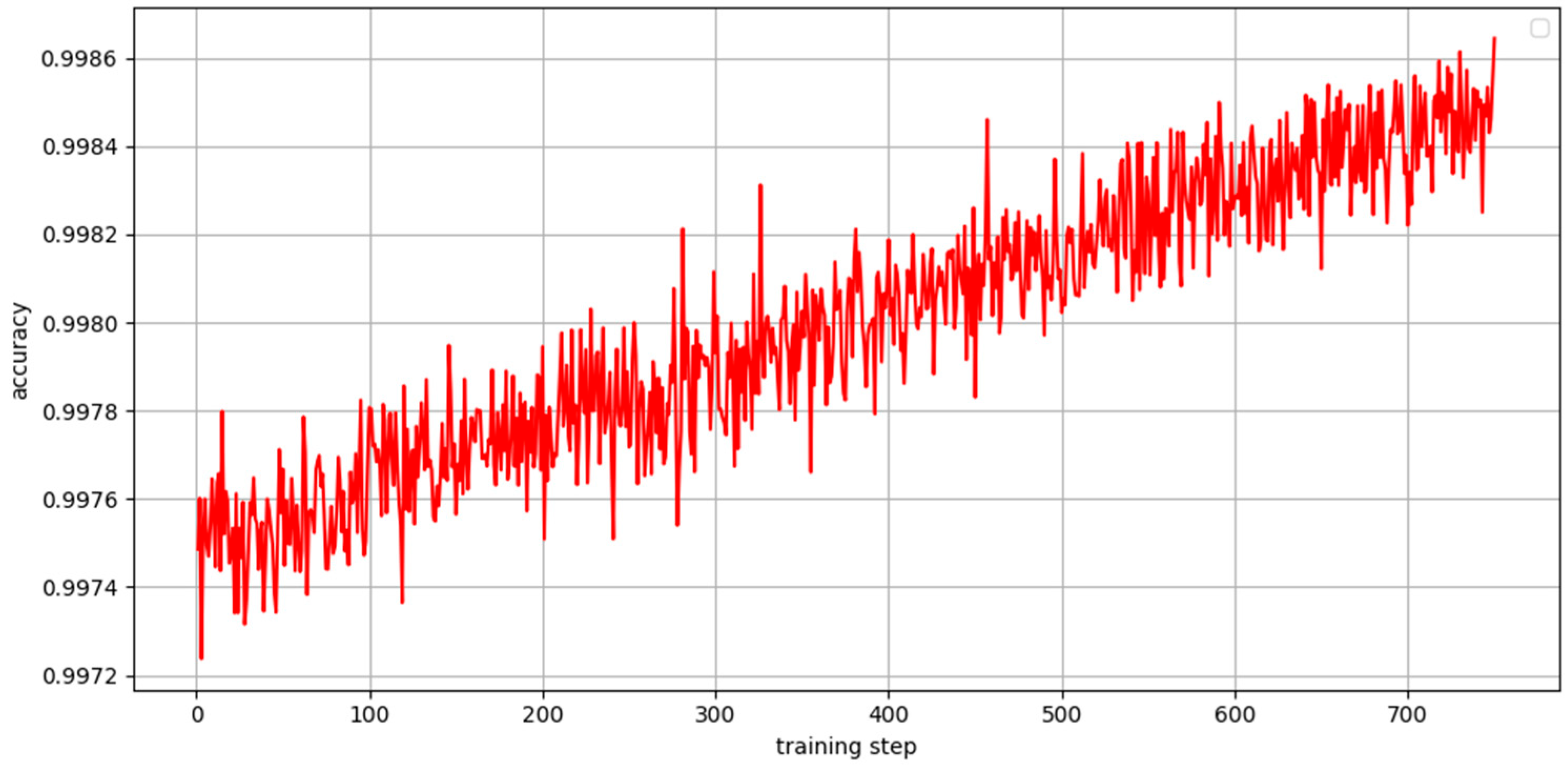
The graph shows the evolution of the model’s accuracy during training, as shown in Figure 11. The Y-axis shows accuracy, and the X-axis shows the training steps. This graph represents the accuracy on the validation set, highlighting how the model improves its ability to correctly classify validation samples.

An upward trend in accuracy is observed as the number of training steps increases. This indicates that the model is progressively learning to make more accurate predictions as the training progresses, which is a good sign that the model is properly adjusting to the task. The fluctuation in the graph could be related to the inherent variability in training, but the overall trend shows a continuous improvement in the model’s ability to make correct predictions.

3.3.3. Confusion Matrix

When building classification models, it is necessary to evaluate their performance. For this purpose, evaluation metrics that capture different aspects of performance are employed, particularly in the context of binary and multiclass classification tasks.

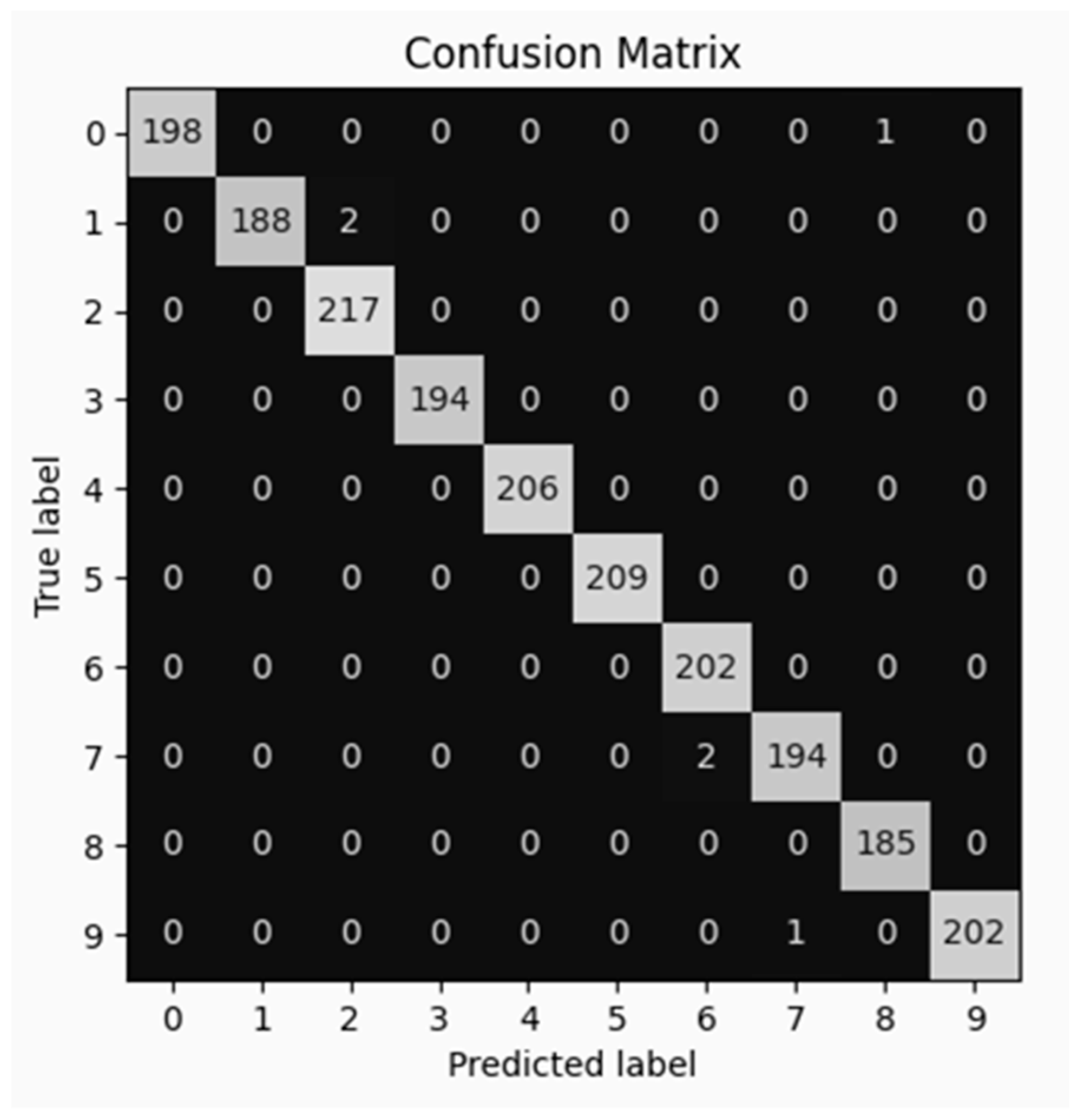
The confusion matrix is an essential tool for evaluating a model’s performance by analyzing correct and incorrect predictions. In this study, the confusion matrix presents the model’s performance in classifying ten diseases from reported symptoms, as shown in Figure 12.

The confusion matrix is organized as follows: the Y-axis corresponds to the true labels, representing the actual diseases in the dataset, while the X-axis corresponds to the labels predicted by the model. Each cell in the matrix indicates the number of instances for which a given predicted label coincides with a true label. The diagonal cells represent correct classifications, where the model accurately identified the corresponding disease. For example, the cell in row 0, column 0, with a value of 198, indicates that the model correctly predicted 198 instances of disease 0.

Cells outside the diagonal represent misclassifications, showing how many times the model predicted a different disease from the true one. For instance, the cell in row 1, column 2, with a value of 2, indicates that disease 2 was incorrectly predicted instead of disease 1.

Overall, the confusion matrix demonstrates good model performance, as most diagonal cells contain high values. Nevertheless, a small degree of confusion is observed among certain classes, particularly diseases with overlapping or similar symptoms, which is a common challenge in classification tasks.

3.3.4. F1 Score

F1 score is a measure that combines the precision and recall of a classification model into a single value. It is mainly used in classification problems, especially when the classes are imbalanced.

It calculates the average between precision and recall, balancing both metrics to provide a more comprehensive view of the model’s performance.

For each class k, the necessary metrics to obtain the F1 score are calculated:

• True positives ($T{P}_k):$

  $$T{P}_k=conf\_matrix[k,k].$$

  (14)

Here, k represents the specific class for which we are calculating the metrics. TP_k is the number of examples that truly belong to class k and that the model correctly classified as class k. This value is located on the diagonal of the confusion matrix, in row k and column k.

• False positives ($F{P}_k):$

  $$F{P}_k={\sum }_{i=0}^{N-1}conf\_matrix[i,k] - T{P}_k.$$

  (15)

In the equation above, i represents the index that goes through all the rows of the matrix for column k. This means we sum up all the predictions made by the model as class k (column k), including both correct and incorrect ones. Then we subtract the true positives TP_k, leaving only the cases that the model predicted as class k but that belong to other classes different from k.

• False Negatives ($F{N}_k):$

  $$F{P}_k={\sum }_{i=0}^{N-1}conf\_matrix[k,j] - T{P}_k.$$

  (16)

Here, j is the index that goes through all the columns of the matrix for row k. This represents the sum of all the actual examples of class k (row k), both those that were correctly classified by the model and those that were misclassified into other classes. By subtracting the true positives TP_k, cases that truly belong to class k are obtained along with those classified into another class, that is, the false negatives.

• Precision (${Precision}_k):$

  $${Precision}_k= {\displaystyle \frac{T{P}_k}{T{P}_k+F{P}_k}}.$$

  (17)

This metric indicates the proportion of predictions the model made as class k that were correct. It is calculated using the previously obtained values of TP_k and FP_k.

• Recall (${Recall}_k):$

  $${Recall}_k={\displaystyle \frac{T{P}_k}{T{P}_k+F{N}_k}}.$$

  (18)

This metric measures the proportion of actual examples of class k that were correctly identified by the model. It is calculated using TP_k and FN_k.

• F1 score (${F1}_k):$

  $${F1}_k=2{\displaystyle \frac{{Precision}_k \left({Recall}_k\right)}{{Precision}_k +{Recall}_k}}.$$

  (19)

The F1 score combines precision and recall into a single metric that balances both values using their harmonic meaning.

A high F1 score value (close to 1) means that the model predicts that class well, both in precision and recall. If any class has a low F1 score, it is a sign that the model has problems with that condition (possibly confusion with others).

The results reflect a high performance of the model in classifying the 10 diseases, as shown in

Table 3. Evaluation Metrics.

Class	Precision	Recall	F1 Score
0 Respiratory allergies	1.0000	0.9950	0.9975
1 Bronchiectasis	1.0000	0.9895	0.9947
2 Chronic bronchitis	0.9857	1.0000	0.9928
3 ischemic heart disease	1.0000	1.0000	1.0000
4 COPD	1.0000	1.0000	1.0000
5 Interstitial lung disease	1.0000	1.0000	1.0000
6 Pulmonary emphysema	0.9902	1.0000	0.9951
7 Laryngitis	0.9948	0.9898	0.9923
8 Vasomotor rhinitis	0.9946	1.0000	0.9973
9 Sinusitis	1.0000	0.9951	0.9975

. For all classes, precision and recall are high, with values close to or equal to 1, indicating that the model correctly classifies most real cases and largely avoids false predictions. For example, in several classes such as 3, 4, and 5, the model achieved perfect precision and recall, meaning it made no errors, false positives, or false negatives during evaluation. In other classes, like 2 and 6, although recall is perfect, precision is slightly less than 1, indicating the model detected all real cases but confused some examples with other classes, generating a few false positives. From a practical perspective, these results are encouraging, as they indicate that the model is capable of accurately classifying the reported symptomatologies.

Furthermore, the good performance of the model is especially relevant in contexts where access to medical specialists is limited or where there is no internet or limited computational resources, as it can serve as a support tool for medical personnel. However, it is important to note that the dataset used is relatively small and limited, which may affect the model’s ability to generalize to more diverse scenarios or different populations. Therefore, increasing the quantity and diversity of available data could further improve the robustness and generalization of the model, enabling more solid and reliable results in real-world settings, as shown in Table 3.

Although this setup does not correspond to a large-scale infrastructure or a multi-GPU cluster, it is suitable for the retraining of a pre-trained large language model (LLM) such as LLaMA 3. This is because the fine-tuning process involves updating a reduced subset of parameters, which requires significantly fewer resources compared to training from scratch.

Training a large model from scratch demands considerable computational resources, generally involving multiple high-performance GPUs operating in parallel over extended periods. In contrast, fine-tuning leverages a previously trained model and adjusts its parameters for specific tasks, reducing both computational load and training time. In this context, a modern GPU like the RTX 4060 Ti provides sufficient performance to carry out this type of fine-tuning without the need for complex or massive infrastructures.

3.4. Inference Time

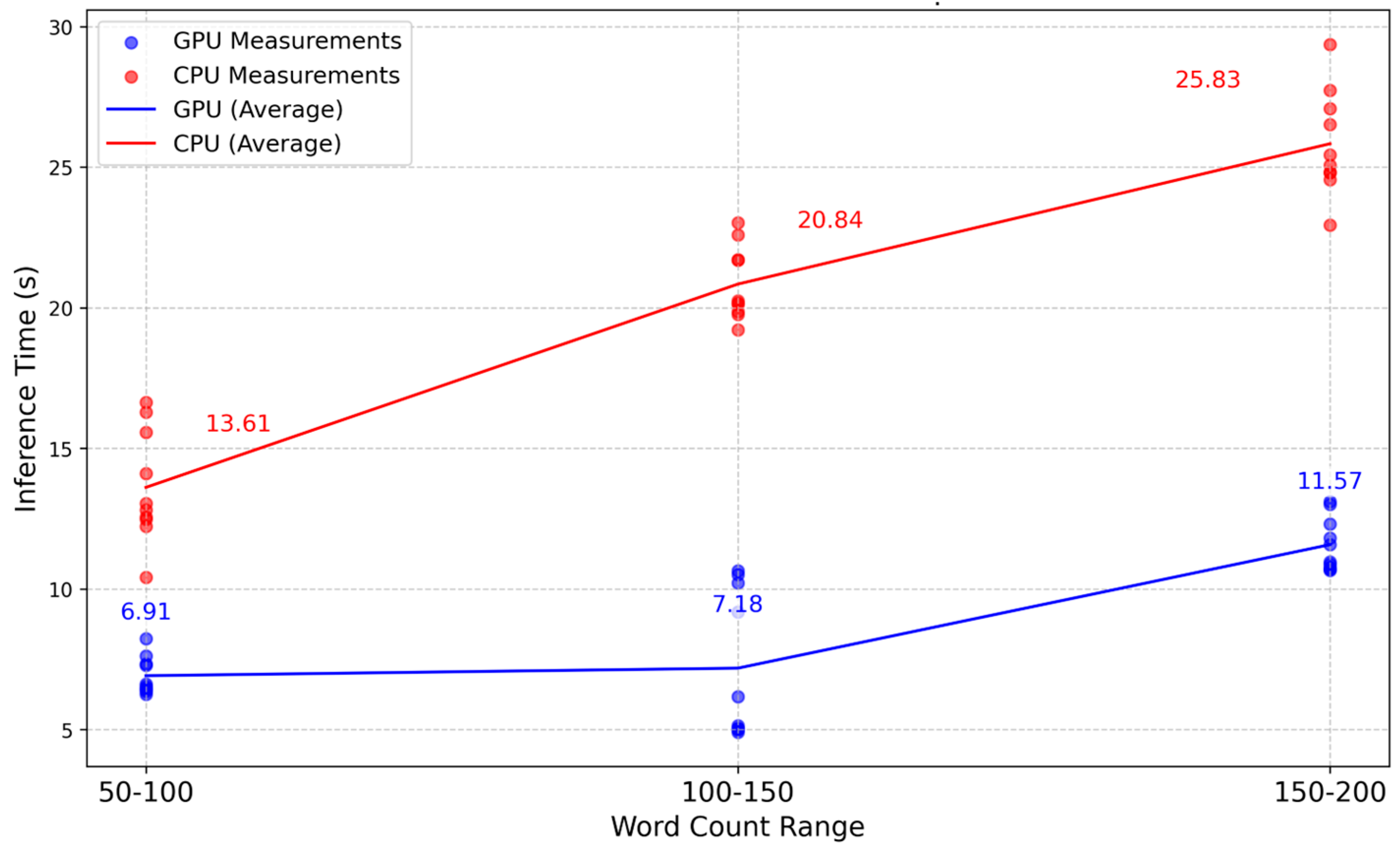
In this project, fine tuning of the LLaMA 3 model was performed using the QLoRA technique to adapt it for a text classification task with 10 labels related to symptomatology caused by environmental pollution. The goal was for the model to identify and classify diseases or conditions based on the symptoms described in the input texts. To evaluate inference performance, texts of different length ranges were selected: 50–100, 100–150, and 150–200 words, and inference times were measured both on CPU and GPU.

The hardware used for the tests included an Intel Core i5 12th Gen CPU and an NVIDIA GeForce RTX 4060 Ti GPU. The results showed that inference on the GPU is significantly faster than on the CPU across all three text length ranges. For example, for texts between 50 and 100 words, the average inference time on the GPU was approximately 6.91 s, while on the CPU it was 13.61 s. As the text length increased, inference times also increased, reaching 11.57 s on the GPU and 25.83 s on the CPU for texts between 150 and 200 words. This pattern indicates that the GPU not only speeds up inference but also scales better with the increased computational load of processing longer texts, as shown in Figure 13.

Using QLoRA for fine-tuning is crucial in this context, as this technique allows the adaptation of large models with only a fraction of the computational resources required for traditional training. This enables robust models such as LLaMA 3 to be tailored for specific tasks without relying on highly specialized or costly hardware, thereby facilitating local execution on moderately capable computers, such as the hardware employed in this study.

This is particularly relevant because the original full version of LLaMA 3 is a very large model, comprising tens of billions of parameters and requiring substantial memory and computational power for execution. Running the unoptimized model without parameter reduction on conventional hardware would be inefficient, or even infeasible, for practical applications due to its high resource demands.

The benefits of fine-tuning with QLoRA therefore extend beyond task-specific model customization, as they also enable local deployment with reasonable inference times and accessible computational resources. This represents a significant advancement for applications in health and research, where fast and reliable solutions with strong privacy guarantees are essential, since sensitive data can remain within the local environment.

In summary, the combination of efficient fine-tuning and the use of accessible hardware enables the deployment of large language models adapted to specific needs, optimizing both performance and computational cost. This development contributes to the democratization of advanced AI models, which were previously restricted to highly specialized and costly infrastructures.

3.5. Comparison with the Base Model

Now, the comparison is made between the fine-tuned model and the base model, which corresponds to LLaMA 3 in its 8-billion-parameter version without any specific adjustment for this task. To evaluate the performance of the base model, a prompt was used in which the reported symptoms are input in natural language text, and the model is asked to classify those symptoms into one of the 10 categories of diseases caused by environmental pollution.

The prompt used was the following:

Text: “Reported symptoms”

Classify the symptoms in the text into:

Respiratory allergies, Bronchiectasis, Chronic bronchitis, Ischemic heart disease, COPD, Interstitial lung disease, Pulmonary emphysema, Chronic laryngitis, Vasomotor rhinitis, Chronic sinusitis.

Answer: “Assigned label”

This approach directly assesses the base model’s capacity to interpret and classify symptoms without prior training or domain-specific adaptation.

The comparison allows measuring the improvement obtained thanks to fine-tuning with QLoRA and how this specialization impacts precision, recall, and F1 score in the classification of these diseases, as shown in

Table 4. Comparison with the base model.

Class	Base Model F1 Score	F1 Score of the Fine-Tuned Model
0 Respiratory allergies	0.7245	0.9975
1 Bronchiectasis	0.8031	0.9947
2 Chronic bronchitis	0.7615	0.9928
3 ischemic heart disease	0.7159	1.0000
4 COPD	0.6698	1.0000
5 Interstitial lung disease	0.7365	1.0000
6 Pulmonary emphysema	0.6242	0.9951
7 Laryngitis	0.7459	0.9923
8 Vasomotor rhinitis	0.7629	0.9973
9 Sinusitis	0.7595	0.9975

. Moreover, this evaluation highlights the importance of adapting general models to specific applications to obtain clinically useful and reliable results.

The results reflect a substantial improvement in the model’s performance after fine-tuning with QLoRA compared to the base model. The fine-tuned model achieves F1 score values very close to 1 across all categories, indicating almost perfect precision and recall in classifying diseases caused by environmental pollution.

It is important to note that the base model was trained on a general-purpose dataset, without specialization in this domain or in the Spanish language, which limits its capacity to accurately interpret the symptomatology specific to this field. In contrast, the fine-tuned model was trained specifically for this task and in Spanish, which substantially contributes to the observed performance improvement.

Furthermore, discrepancies in performance may also stem from differences in labeling criteria and language representation between the base model and the new model. The dataset used for fine-tuning contains sentences and expressions similar in style to the test samples, which favors the model’s performance in the current evaluations.

However, introducing more varied sentence structures or linguistic styles may influence the results. This suggests that, although the findings are very promising, the model’s robustness could be further improved through the use of larger, more diverse, and more representative datasets reflecting real-world symptomatology.

3.6. Language

In

Table 5. Descriptions of Symptoms of Linguistic Variations.

Description	Classification	Analysis
Te escribo porke la neta ando bien jodido del pecho, Ai rato me falta el aire hasta pa ir a la tienda y me canzo bien rapido. la tos no me deja, sobre todo en las mañanas y siempre estoy escupiendo mocos güeros o amarillos bien feos. Abeces se me hace como un silbidito en el pecho, y asta me duele cuando respiro hondo. Ando todo cansado hasta pa subir un escalón y ya ni ganas de comer tengo. Se me ponen morados los labios y las uñas, y la neta me asusto, yo fumaba un buen antes pero ahorita ya ni un cigarro puedo	EPOC	porke—porque canzo—cansó abeces—a veces astá—hasta La neta—La Verdad Ando bien jodido—Estoy muy enfermo Un buen—mucho Mocos gueros—Flemas amariillas

, an example of reported symptomatology is presented, showing how informal descriptions and linguistic variability, such as spelling mistakes and local idioms, were processed by the model. Each example includes the input text with its respective spelling corrections, colloquial words typical of central Mexico, and the model’s classification based on the reported symptoms.

This example shows how people from the central region of Mexico use very colloquial language and spelling variations to describe their symptoms. Some of the expressions used, such as “la neta,” “jodido,” or “un buen,” are common in everyday speech among the Mexican population, and they are translated informally to reflect how a person might describe their discomforts without worrying about grammatical correctness or the formal use of language.

Despite these variations, the model was able to correctly classify the symptoms as related to COPD (Chronic Obstructive Pulmonary Disease), demonstrating that, having been trained with a dataset that includes linguistic variability and common errors, the model can effectively handle these “real language” cases and not just formal ones.

One reason the model can correctly manage these examples is attributable to the Transformer architecture, which enables the processing of complete text sequences and the modeling of global contextual dependencies among words and phrases. Through its self-attention mechanism, the Transformer assigns differential weights to relevant tokens, even in the presence of misspellings or colloquial expressions. This capability allows the model to capture linguistic variability without losing semantic meaning, thereby improving its adaptability to the diverse language styles used by participants.

3.7. Graphical User Interface (GUI)

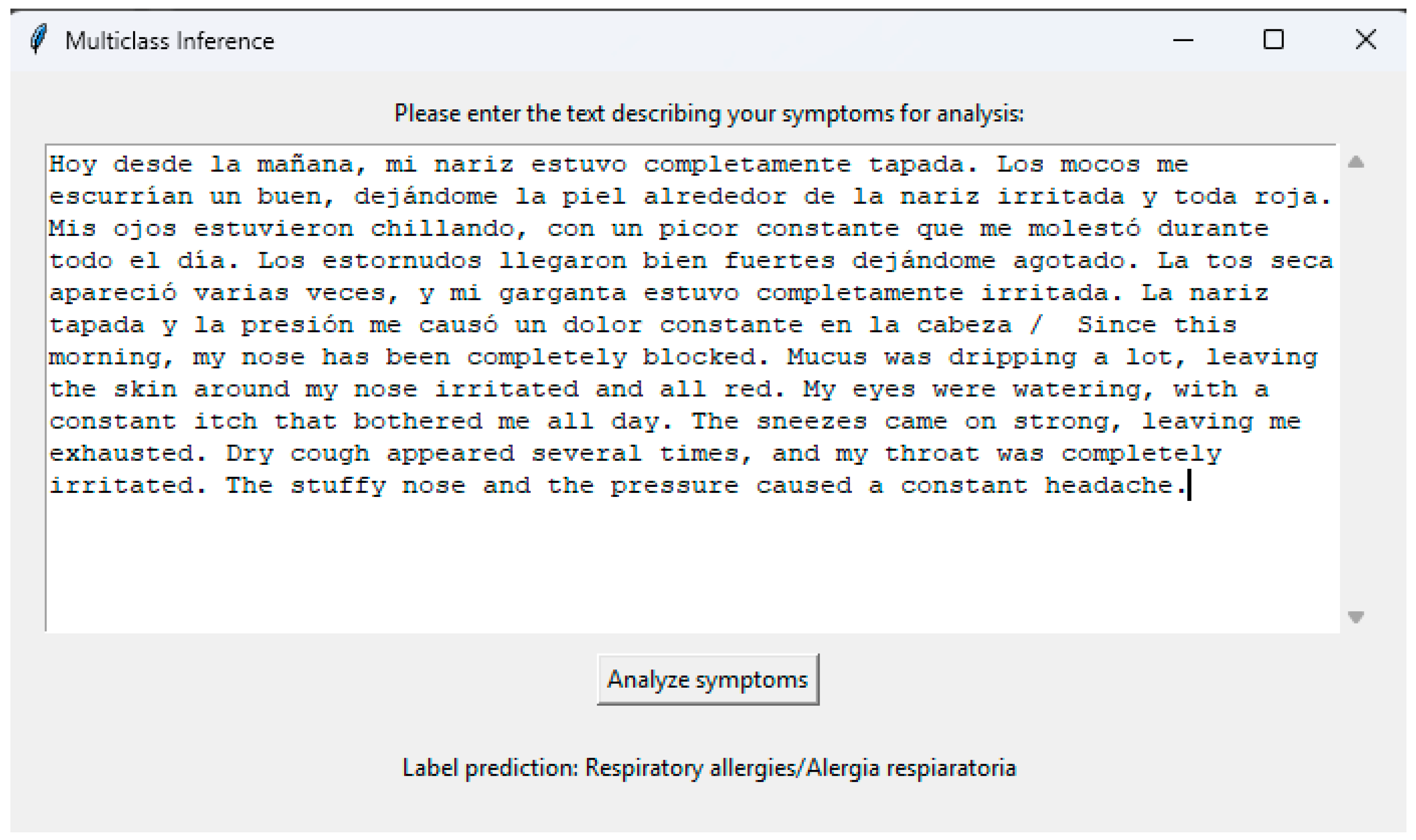
As part of the final implementation of the system, a Graphical User Interface (GUI) was developed using Tkinter, which allows users to easily interact with the model and obtain predictions about diseases based on the symptoms they introduce.

The interface has an accessible design. The user can enter a text describing their symptoms in a text box, and by clicking a prediction button, the system processes the input through the fine-tuned and quantized LLaMA 3 model. Based on the symptoms described, the model predicts the associated disease and displays the result in the same window in a clear and understandable way.

Although the text entered by the user may contain spelling errors, variations in language use, or even code-switching, as seen in Figure 14, the system is capable of accurately detecting and analyzing the symptoms thanks to a robust pre-trained language model behind the interface, which is LLaMA 3.

This pre-trained model already has a broad and general understanding of natural language, enabling it to comprehend texts with different styles, common errors, and diverse expressions. Additionally, to improve accuracy in our specific case, the model has been fine-tuned using a dataset specially constructed for our environment. This dataset contains real examples of medical terminology adapted to the region and common situations.

Thanks to this fine-tuning, the model not only recognizes common words and expressions but also linguistic combinations unique to the local context or medical field, even if they contain errors or variations

3.8. Qualitative Error Analysis

Text Reported by the User:

“Mira, tengo tos casi diario sobre todo en la mañana. Siempre ando escupiendo un buen de moco y neta me siento bien cansado cuando hago cualquier esfuerzo. Me falta el aire asta para subirme las escaleras o cuando intento acer ejercicio y a veces siento komo si algo me apretara el pecho y asta escucho un silbido cuando respiro. Esto ya me pasa cada vez mas y me molesta.”

Model Prediction:

• Chronic bronchitis
• COPD (Chronic Obstructive Pulmonary Disease)

Similarities Between COPD and Chronic Bronchitis. Chronic Obstructive Pulmonary Disease (COPD) and Chronic Bronchitis share several clinical manifestations, which complicates accurate classification in cases with overlapping symptoms. Both conditions are characterized by chronic cough, excessive sputum production, dyspnea on exertion, wheezing, and chest tightness. This overlap makes it challenging for the model to differentiate between the two diseases based solely on reported symptoms.

Ambiguous Description. In the analyzed case, the patient reported general symptoms such as dyspnea, cough, and excessive sputum, but did not provide sufficient detail to allow a clear distinction between COPD and Chronic Bronchitis. In particular, the absence of information regarding symptom duration and clinical history limited the model’s ability to achieve a more precise classification.

Lack of Additional Data. The primary distinction between COPD and Chronic Bronchitis lies in disease progression and etiology: COPD is a progressive condition associated with long-term lung damage due to exposure to irritants (e.g., environmental pollutants), whereas Chronic Bronchitis specifically refers to chronic airway inflammation. The absence of data on exposure to pollutants hinders the model’s ability to differentiate between these diseases, since both are pollution-related but affect the respiratory system in different ways.

Disclaimer. It is important to emphasize that this analysis and the model’s predictions do not constitute a medical diagnosis. The model functions as a decision-support tool for classifying reported symptoms and suggesting potential conditions; however, it does not replace clinical judgment.

4. Future Work

Future work will focus on adapting the fine-tuned LLaMA 3 model for clinical use by addressing ethical, regulatory, and practical considerations. This includes ensuring responsible use by positioning the model strictly as a decision-support tool rather than a substitute for medical diagnosis, incorporating safeguards to avoid biases against underrepresented groups, and guaranteeing robust performance across diverse linguistic and regional contexts. Compliance with data protection frameworks such as GDPR and the Federal Law on Protection of Personal Data in Mexico will be essential, requiring strict anonymization and secure handling of clinical information. To enhance trust and safety, transparency and explainability techniques (e.g., SHAP values and attention maps) will be integrated, enabling healthcare professionals to interpret the factors driving model predictions. In parallel, future efforts will prioritize expanding and diversifying the dataset to cover broader demographic, linguistic, and clinical contexts, thereby improving generalization and the handling of ambiguous or complex cases. Ultimately, these advances will allow the development of a clinical-oriented version of the model designed to support healthcare professionals as a reliable decision-support system, always under medical supervision.

5. Conclusions

In this study, it became evident that individuals across different ages, genders, and educational backgrounds employ a wide range of words and expressions to describe common ailments, introducing significant linguistic variability, including synonyms, local idioms, spelling errors, and colloquial expressions. This linguistic diversity enabled the construction of a representative dataset that captures the nuances and meanings users assign to their symptoms, which is crucial for training a model capable of accurately interpreting and classifying varied descriptions.

This linguistic diversity enhances model accuracy by capturing the diverse ways in which symptoms are described and provides the foundation for constructing a balanced and realistic dataset suitable for training models capable of generalizing effectively across individuals with diverse forms of expression. Accordingly, the dataset used in this study was built not only from structured data but also from an appreciation of how language reflects the human experience of illness and discomfort in informal, everyday contexts in the Spanish language of central Mexico.

This study demonstrates that effective fine-tuning of a large model such as LLaMA 3 can be achieved using the QLoRA technique, which combines quantization with low-rank adaptation, thereby significantly reducing computational and memory requirements. This approach enables training and deployment of models with billions of parameters on accessible hardware, facilitating their use in clinical applications within environments with limited infrastructure and potentially making them available to a broader range of users. Through quantization, the fine-tuned model can be executed locally even on devices with constrained resources, without reliance on complex infrastructures or large-scale computing centers. This greatly enhances the feasibility of implementation in remote regions or clinics with limited technical capabilities, expanding the potential impact of artificial intelligence in public health. The trained model achieved high accuracy in classifying ten diseases associated with environmental pollution, demonstrating balanced performance across classes without significant biases. Although the confusion matrix revealed a small degree of misclassification among diseases with overlapping symptoms—a common challenge in clinical text-based tasks—the overall results indicate strong predictive capacity and robustness.

The use of a balanced dataset, together with preprocessing steps such as normalization, noise removal, tokenization, and embedding generation, was essential to ensuring stable training and effective model generalization. Data diversity, including the incorporation of synonyms and spelling errors, further enhanced system robustness. The results indicate that the model can serve as a valuable tool for classifying diseases associated with environmental pollution based on textual symptom descriptions, particularly in regions with limited access to medical specialists. Moreover, the development of a graphical interface facilitates its integration into clinical and public health settings, promoting accessibility and ease of implementation.

Nevertheless, the model’s effectiveness remains dependent on the quality and representativeness of the input data. The observed misclassifications among diseases with overlapping symptoms underscores the need for continued algorithmic refinement and further expansion of dataset diversity. Additionally, given that the model was trained exclusively on Spanish-language texts, its application in other linguistic contexts would require additional adaptation.

References

1. Goldsmith, J.R. Environmental Pollution and Its Effects on Health; Springer: Berlin/Heidelberg, Germany, 2018. [Google Scholar]
2. Jurafsky, D.; Martin, J.H. Speech and Language Processing, 3rd ed.; Pearson: London, UK, 2020. [Google Scholar]
3. Topol, E.J. High-performance medicine: The convergence of human and artificial intelligence. Nat. Med. 2019, 25, 44–56. [Google Scholar] [CrossRef] [PubMed]
4. Al Nazi, Z.; Peng, W. Large language models in healthcare and medical domain: A review. Informatics 2024, 11, 57. [Google Scholar] [CrossRef]
5. Brown, T.; Mann, B.; Ryder, N.; Subbiah, M.; Kaplan, J.D.; Dhariwal, P.; Neelakantan, A.; Shyam, P.; Sastry, G.; Askell, A.; et al. Language models are few-shot learners. Adv. Neural Inf. Process. Syst. 2020, 33, 1877–1901. [Google Scholar]
6. Petroni, F.; Rocktäschel, T.; Lewis, P.; Bakhtin, A.; Wu, Y.; Miller, A.H.; Riedel, S. Language models as knowledge bases? arXiv 2019, arXiv:1909.01066. [Google Scholar] [CrossRef]
7. Touvron, H.; Lavril, T.; Izacard, G.; Martinet, X.; Lachaux, M.A.; Lacroix, T.; Rozière, B.; Goyal, N.; Hambro, E.; Azhar, F.; et al. LLaMA: Open and efficient foundation language models. arXiv 2023, arXiv:2302.13971. [Google Scholar] [CrossRef]
8. Radford, A.; Narasimhan, K.; Salimans, T.; Sutskever, I. Improving Language Understanding by Generative Pre-Training. 2018. Available online: https://cdn.openai.com/research-covers/language-unsupervised/language_understanding_paper.pdf (accessed on 17 July 2025).
9. Chowdhery, A.; Narang, S.; Devlin, J.; Bosma, M.; Mishra, G.; Roberts, A.; Barham, P.; Chung, H.W.; Sutton, C.; Gehrmann, S.; et al. Palm: Scaling language modeling with pathways. arXiv 2022, arXiv:2204.02311. [Google Scholar] [CrossRef]
10. Alsentzer, E.; Murphy, J.; Boag, W.; Weng, W.-H.; Jin, D.; Naumann, T.; McDermott, M. Publicly Available Clinical BERT Embeddings. In Proceedings of the 2nd Clinical Natural Language Processing Workshop, Minneapolis, MN, USA, 7 June 2019. [Google Scholar]
11. Strubell, E.; Ganesh, A.; McCallum, A. Energy and Policy Considerations for Deep Learning in NLP. In Proceedings of the ACL 2019, Florence, Italy, 1–6 July 2019. [Google Scholar]
12. Patterson, D.; Gonzalez, J.; Le, Q.; Liang, C.; Munguia, L.M.; Rothchild, D.; So, D. Carbon Emissions and Large Neural Network Training. arXiv 2021, arXiv:2104.10350. [Google Scholar] [CrossRef]
13. Hu, E.J.; Shen, Y.; Wallis, P.; Allen-Zhu, Z.; Li, Y.; Wang, S.; Wang, L.; Chen, W.; Chen, Y.; Li, H. LoRA: Low-Rank Adaptation of Large Language Models. arXiv 2021, arXiv:2106.09685. [Google Scholar]
14. Dettmers, T.; Lewis, M.; Belkada, Y.; Zettlemoyer, L.; Su, J. QLoRA: Efficient Finetuning of Quantized LLMs. arXiv 2023, arXiv:2305.14314. [Google Scholar] [CrossRef]
15. Peng, Y.; Yan, S.; Lu, Z. Transfer Learning in Biomedical Natural Language Processing: An Evaluation of BERT and ELMo on Ten Benchmarking Datasets. In Proceedings of the 18th BioNLP Workshop and Shared Task, Florence, Italy, 1 August 2019; pp. 58–65. [Google Scholar] [CrossRef]
16. Bousquet, J.; Khaltaev, N.; Cruz, A.A.; Denburg, J.; Fokkens, W.J.; Togias, A.; Zuberbier, T. Allergic diseases and asthma in the era of environmental pollution: A global perspective. World Allergy Organ. J. 2020, 13, 100118. [Google Scholar]
17. Vaswani, A.; Shazeer, N.; Parmar, N.; Uszkoreit, J.; Jones, L.; Gomez, A.N.; Kaiser, Ł.; Polosukhin, I. Attention is all you need. Adv. Neural Inf. Process. Syst. 2017, 30, 5998–6008. [Google Scholar]
18. Dufter, P.; Schmitt, M.; Schütze, H. Position Information in Transformers: An Overview. Comput. Linguist. 2022, 48, 733–763. [Google Scholar] [CrossRef]
19. Li, Y. Theoretical Analysis of Positional Encodings in Transformer Models: Impact on Expressiveness and Generalization. arXiv 2025, arXiv:2506.06398. [Google Scholar] [CrossRef]
20. Zhou, D.; Shi, Y.; Kang, B.; Yu, W.; Jiang, Z.; Li, Y.; Jin, X.; Hou, Q.; Feng, J. Refiner: Refining self-attention for vision transformers. arXiv 2021, arXiv:2106.03714. [Google Scholar] [CrossRef]
21. Al Nazi, Z.; Mashrur, F.R.; Islam, M.A.; Saha, S. Fibro-cosanet: Pulmonary fibrosis prognosis prediction using a convolutional self attention network. Phys. Med. Biol. 2021, 66, 225013. [Google Scholar] [CrossRef] [PubMed]
22. Hao, Y.; Dong, L.; Wei, F.; Xu, K. Self-attention attribution: Interpreting information interactions inside transformer. In Proceedings of the AAAI Conference on Artificial Intelligence, Virtual, 2–9 February 2021; Volume 35, pp. 12963–12971. [Google Scholar]
Figure 1. General diagram of the research process.
Applsci 15 09772 g001
Figure 2. Distribution of participants in terms of gender and age.
Applsci 15 09772 g002
Figure 3. Text to vector conversion process.
Applsci 15 09772 g003
Figure 4. Vector containing embedding and positional information.
Applsci 15 09772 g004
Figure 5. Decomposition of the weight matrix in LoRA using low-rank matrices Matrix decomposition.
Applsci 15 09772 g005
Figure 6. Number of examples in sentences with a certain range of words.
Applsci 15 09772 g006
Figure 7. Average number of words for each class.
Applsci 15 09772 g007
Figure 8. Number of examples for each class.
Applsci 15 09772 g008
Figure 9. Relationships between embedding vectors in space.
Applsci 15 09772 g009
Figure 10. Evolution of the loss during training.
Applsci 15 09772 g010
Figure 11. Evolution of accuracy.
Applsci 15 09772 g011
Figure 12. Confusion matrix.
Applsci 15 09772 g012
Figure 13. Graph of Inference time.
Applsci 15 09772 g013
Figure 14. Inference illustrated using the GUI.
Applsci 15 09772 g014