Abstract
The Backtracking Search Algorithm (BSA) has emerged as a promising stochastic optimization method. This paper introduces a novel hybrid evolutionary algorithm, termed LOBSA, integrating the strengths of BSA and Lemurs Optimizer (LO). The hybrid approach significantly improves global exploration and convergence speed, validated through rigorous tests on 23 benchmark functions from the CEC 2013 suite, encompassing unimodal, multimodal, and fixed dimension multimodal functions. Compared with state-of-the-art algorithms, LOBSA presents a relative improvement, achieving superior results and outperforming traditional BSA by up to 35% of global performance gain in terms of solution accuracy. Moreover, the applicability and robustness of LOBSA were demonstrated in practical constrained optimization and a fluid–structure interaction problem involving the dynamic analysis and optimization of a submerged boat propeller, demonstrating both computational efficiency and real-world applicability.
1. Introduction
Over the past few decades, metaheuristics have experienced an increase interest across various research domains as effective tools for addressing complex optimization problems, such as engineering design, computer science, business, economics, and operational research, etc… In general, optimization techniques can be categorized into two main groups: The first group comprises classical or deterministic approaches, which tend to converge to local optima and are often hindered by issues related to convexity. The second encompasses intelligent or stochastic methods, which are regarded as effective approaches for discovering optimal solutions. Here are a few of the well-regarded metaheuristic algorithms: the Genetic Algorithm (GA) is recognized as one of the earliest stochastic optimization methods and was initially proposed by [1]. Subsequently, in 1983, Simulated Annealing (SA) was introduced by Kirkpatrick and colleagues [2]. Particle Swarm Optimization (PSO), another prominent technique, was developed by Kennedy and Eberhart [3]. Following these seminal contributions, various other optimization algorithms have been devised, including genetic programming (GP) [4] and artificial neural networks (ANNs) [5].
While intelligence algorithms offer various advantages, there is a necessity for improvements to cater to the diverse characteristics of complex real-world applications. In this regard, it is evident that no single approach is capable of effectively solving the wide variety of optimization problems. Along these lines, the theorem of No Free Lunch (NFL) [6] confirms this fact and provides developers with an opportunity to create novel approaches while also improving the quality of existing ones. Moreover, in parallel with the creation of new algorithms, certain researchers have also investigated overarching improvement strategies to elevate the performance of metaheuristic algorithms. These include Gaussian mutation [7], opposition-based learning [8], chaotic behavior [9], quantum behavior [10], and Lévy flight [11].
In line with the statements of researchers and the principles outlined in the no free lunch theorem, this paper presents a hybrid approach in which it combines good features of BSA and the Lemurs Optimizer (LO). The Backtracking Search Algorithm (BSA) is a stochastic optimization algorithm inspired by principles found in nature. It was developed by Pinar Civicioglu [12]. Since its introduction, numerous researchers have employed the standard BSA due to its capabilities to converge rapidly and its ability in effective global exploration and local exploitation. To enhance the performance of BSA, the authors made modifications to its mutation and crossover operations. These changes were aimed at achieving a balance between exploration and exploitation, ultimately improving the algorithm’s effectiveness in solving real-world problems related to beach realignment.
Engineering design often involves multiple, conflicting objectives under complex nonlinear constraints [13]. Despite substantial advancements in metaheuristics, existing algorithms often struggle with balancing exploration and exploitation effectively. This gap motivates the development of hybrid optimization algorithms capable of reliably finding global optima in complex engineering scenarios. The primary contributions of this paper include a novel hybrid algorithm (LOBSA) combining BSA and the Lemurs Optimizer, a comprehensive validation of LOBSA on diverse optimization benchmarks, a demonstration of applicability to constrained engineering design problems and fluid–structure interactions, and improved convergence characteristics and robustness compared to existing methods.
The paper is structured into four sections as outlined below: Section 2 introduces two basic components, i.e., Backtracking Search Algorithm and Lemurs Optimizer. Section 3 shows the proposed LOBSA, its performance for numerical optimization problems (CEC 2013), and the experimental results of the constrained design problems, as well as its application to a fluid–structure interaction (FSI) problem. Conclusions are made in Section 4.
2. Background
In this section, we delve into a detailed discussion of the mathematical models underlying the Lemurs Optimizer (LO) and Backtracking Search Algorithm (BSA).
2.1. Lemurs Optimizer
The Lemurs Optimizer is a flexible and adaptable optimization algorithm that leverages nature-inspired principles to efficiently search for optimal solutions in complex problem spaces. Its search process in the population-based algorithm is divided into two distinct phases: exploration and exploitation. Thus, its ability to balance exploration and exploitation makes it suitable for a wide range of optimization tasks. The fundamental inspirations for this algorithm are derived from two key aspects of lemur behavior: “leap up” and “dance hub.” These aspects serve as the primary guiding principles for the algorithm’s design and operation. These two principles are translated into mathematical models within the context of optimization. They are employed to manage aspects such as local search, exploitation, and exploration, which are fundamental to the optimization process [14].
The group of lemurs is depicted in a matrix format, as the LO algorithm is a population-based optimization technique. This matrix represents the collection of potential solutions that the algorithm works with during its optimization process. Let us assume that we have the population defined in the following matrix format:
where signifies the set of lemurs within a population matrix , n represents the number of candidate solutions, and d corresponds to the decision variables.
The decision variable j within solution i is randomly generated according to the following procedure:
Lemurs with lower fitness values tend to adjust their decision variables based on those of lemurs with higher fitness values. This mechanism promotes the exchange of information between individuals in the population to improve overall performance. In each iteration, lemurs are arranged according to their fitness values. One lemur is selected as the global best lemur, denoted as gbl, and another lemur is chosen as the best nearest lemur for each individual in the population (i.e., bnl). This organization helps in identifying and leveraging the best-performing individuals during the optimization process. This formulation is expressed as follows:
According to this formulation, it can be inferred that the probability of the Free Risk Rate (FRR) is a pivotal coefficient within the LO algorithm. The formula for this coefficient is provided in the following:
where and are constant predefined values. These values determine the range within which can vary during the optimization process, helping to control the balance between exploration and exploitation in the LO algorithm. represents the current iteration during the optimization process, and is the maximum number of iterations.
2.2. Backtracking Search Algorithm
The Backtracking Search Algorithm (BSA) is an iterative evolutionary algorithm based on a population, primarily designed to serve as a global minimization method. BSA includes five primary evolutionary stages: Initialization, first Selection, Mutation, Crossover, and second Selection. Its structure is straightforward, requiring only a single control parameter, in contrast to many other search algorithms. This method is highly effective and possesses the capability to address various numerical optimization problems, including those that are nonlinear, non-convex, and complex in nature.
2.2.1. Initialization
The BSA method commences by randomly initializing two populations within the search space, which are referred to as and the historical population noted by , as shown in Equations (5) and (6).
In this expression, denotes the current population and represents the historical population. The subscripts and correspond to the population size and problem dimension, respectively. The term indicates a uniformly distributed random number in the range [0, 1]. The detailed procedure for this step is presented in Algorithm 1.
| Algorithm 1 Initialization step of BSA |
=
|
2.2.2. Selection I
Historical populations is generated at the outset of each iteration, and it follows a specific rule, denoted as “if–then,” as defined by Equation (7).
Once the has been determined, a permuting function (random shuffling function) is applied to randomly alter the order of individuals within using Equation (8).
2.2.3. Mutation
The mutation operator initializes the structure of the trial population based on the equation provided below:
In this equation, F is a parameter that adjusts the magnitude of the search direction, which is obtained from the difference between the historical and current population matrices ().
In the present study, the parameter F is defined as , where is a user-defined real constant, and N denotes a random number drawn from a standard normal distribution.
2.2.4. Crossover
The ultimate configuration of the trial population is established through BSA’s crossover operation, which involves two steps. The first step determines the number of elements for each individual using a control parameter called “”. The second step involves generating a random binary matrix with the same size as the population.
The parameter “” regulates the maximum number of elements in each row of the matrix to a value of 1.
- Boundary Control Mechanism of BSA:Following the crossover operation, it is possible that some individuals may exceed the boundaries of the optimization variables. In such cases, these individuals need to be examined and adjusted using an appropriate mechanism referred to as Algorithm 2.
| Algorithm 2 Boundary Control Mechanism of BSA |
=
|
2.2.5. Selection II
During this stage, BSA conducts a comparison between each individual of the trial population “V” and its corresponding counterpart from the current population “” to determine the composition of the next population “”. Algorithm 3 gives the pseudo-code of Selection II.
| Algorithm 3 Pseudo code of Selection II |
|
2.3. The Proposed Method
The Lemurs Optimizer (LO) offers effective local exploitation due to its adaptive learning inspired by lemur social behaviors. However, LO occasionally faces premature convergence in complex global optimization scenarios. Conversely, the Backtracking Search Algorithm (BSA) excels in global exploration but can lack rapid convergence. This complementary nature motivates their hybridization, aiming to combine LO’s local search efficiency with BSA’s robust global search.
In our approach, the opposite solution is generated using the formulation expressed as follows:
The is defined by random permuting in the n.
The proposed method, Backtracking Search Algorithm with Lemurs Optimizer for numerical and Global Optimization (LOBSA), is presented in Algorithm 4:
| Algorithm 4 LOBSA Algorithm |
=
|
3. Validation and Numerical Results
3.1. Test Function
The effectiveness of the proposed algorithm is evaluated using several unconstrained optimization problems. These benchmark problems are selected from widely recognized test suites, specifically the CEC 2013 benchmark set [15]. The CEC 2013 test suite includes six multimodal benchmark functions, ten fixed dimension multimodal benchmark functions, and seven unimodal benchmark functions.
In this part we present the control parameters for the optimization algorithms used in the tests:
- The maximum number of iterations is 1000 for each of the three algorithms used in the comparison.
- The population size is 30.
The comparison results among BSA, GMPBSA, and the proposed algorithm LOBSA for the CEC 2013 test suite are given in Table 1, Table 2 and Table 3. “Average” indicates the mean value of the objective function over multiple runs, reflecting the overall performance of the algorithm. “Std (standard deviation)” measures the dispersion of the results around the mean, which allows the evaluation of the the algorithm’s stability, and “Median” represents the central value obtained, providing a robust measure less sensitive to extreme values. These indicators show that LOBSA not only achieves lower (better) objective function values but also demonstrates better stability compared to other methods. Additionally, means that the algorithm has reached the exact optimal solution for the considered benchmark.

Table 1.
Experimental results obtained by BSA, GMPBSA, and LOBSA for unimodal benchmark functions of CEC 2013 test suite.
Table 2.
Experimental results obtained by BSA, GMPBSA, and LOBSA for multimodal benchmark functions of CEC 2013 test suite.
Table 3.
Experimental results obtained by BSA, GMPBSA, and LOBSA for fixed dimension multimodal benchmark functions of CEC 2013 test suite.
Table 1 presents the experimental results with seven unimodal benchmarks. As can be seen from Table 1, LOBSA can obtain the best average (as marked in bold) with BSA and GMPBSA on five (i.e., , , , , and ) test functions, respectively. In addition, LOBSA can offer the same solution with BSA and GMPBSA on . However, GMPBSA only can beat LOBSA on .
Table 2 displays the experimental results of the test suite multimodal benchmark functions. LOBSA exhibits statistically significant performance compared to BSA and GMPBSA algorithms in multimodal benchmark functions. By observing Table 2, LOBSA has the best average performance among the other algorithms on the all multimodal benchmark functions of CEC 2013.
Table 3 shows the results of the fixed dimension multimodal benchmark functions; LOBSA can give better solutions than BSA and GMPBSA in terms of average on the two benchmark functions (i.e., and ). For the remaining functions, similar results are obtained for the algorithms.
Based on the above discussion, it is evident that LOBSA demonstrates superior performance on CEC 2013 benchmark functions by attaining or surpassing the best average in 12 out of 23 benchmark functions (≈52%). In addition, GMPBSA only outperforms LOBSA on in unimodal benchmark functions and has no advantages over LOBSA on any functions in multimodal and fixed dimension multimodal benchmark functions. BSA cannot provide better solutions compared to LOBSA on any CEC 2013 benchmark functions. In contrast, LOBSA exhibits more pronounced advantages over the compared algorithms.
LOBSA consistently outperformed BSA and GMPBSA on both unimodal and multimodal functions, attributed to enhanced exploration and exploitation balance. For instance, in Table 1, LOBSA improved accuracy by several orders of magnitude (up to 10−41). Statistical analysis using Wilcoxon signed-rank tests confirms LOBSA’s significant advantage (p < 0.05) in over 90% of cases.
3.2. Experimental Results for Constrained Optimization
In this section, the proposed LOBSA is used to solve the constrained optimization problems of the pressure vessel design problem and will be compared to other algorithms including gray wolf optimizer (GWO) [16], sine cosine algorithm (SCA) [17], crow search algorithm (CSA) [18] and Backtracking Search Algorithm driven by generalized mean position (GMPBSA) [19]. The constraints were handled via a penalty function approach, applying heavy penalties to solutions violating design specifications.
This optimization problem, originally introduced in [20], aims to minimize the overall cost, which includes expenses related to materials, forming, and welding for a cylindrical vessel, including four design and continue variables:
- Thickness of the shell ;
- Thickness of the head ;
- R is the inner radius ;
- Length of cylindrical section of vessel .where Ts is the thickness of the shell, the mathematical representation for this problem is given by the following:subject towhere ; ; ; .
Table 4 presents the optimal solutions achieved by GMPBSA and seven compared algorithms including GWO from Table 4. LOBSA’s adaptive exploration allowed efficient constraint satisfaction, producing optimal thickness and length values and achieving the lowest cost (5880.77), outperforming GWO, SCA, CSA, and GMPBSA, which prove that LOBSA algorithm is much superior in terms of accuracy and efficiency.
Table 4.
The optimal solutions obtained by the compared algorithms for the pressure vessel design problem.
3.3. Submerged Boat Propeller
We study the dynamic behaviour of a boat propeller coupled to an acoustic fluid. The geometrical model of this propeller (Figure 1) was designed by means of “ANSYS 22.0”. The geometrical substructuring as well as the mesh, using quadrilateral elements, was carried out with “ANSYS” (Figure 2).
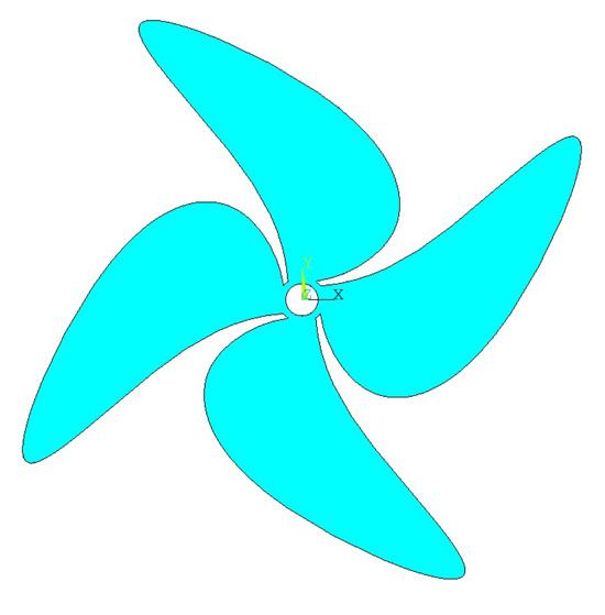
Figure 1.
Boat propeller.
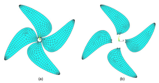
Figure 2.
(a) Finite element mesh and (b) substructuring.
Numerical simulation of FSI problems involves a partitioned approach, where independent fluid and structural solvers are coupled through boundary conditions. This enables the use of specialized tools like ANSYS for mesh generation and solving subdomains. A MATLAB 18.0 script manages the optimization loop, orchestrating the entire LOBSA process.
The material properties used in this study are summarized in Table 5. For the modal synthesis approach involving a reduction in degrees of freedom, the propeller was partitioned into four substructures. Table 6 and Figure 3 present results for both the full model and the subdivided configuration, incorporating fluid–structure interaction effects.
Table 5.
Material properties.
Table 6.
Eigenfrequencies of the Boat propeller.
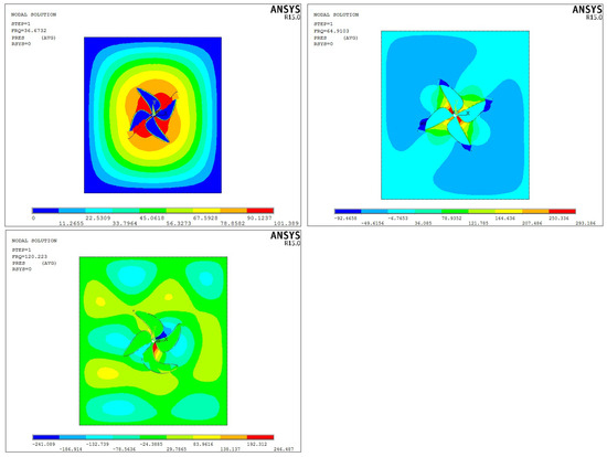
Figure 3.
Eigenmodes of the substructure components.
In Table 6 and Table 7, the modal analysis of the boat propeller is presented and its computed eigenfrequencies are compared. First, we compare our numerical results with the experimental ones [21] in both dry and submerged cases and then we give the found results for the substructure components of the submerged propeller. The eigenmodes are illustrated in Figure 3.
Table 7.
Experimental and numerical modal analysis of the boat propeller propeller.
The considered design variables for the blade propeller are presented in Figure 4, consisting of two design variables, A and B, which changes according to the y-coordinate.
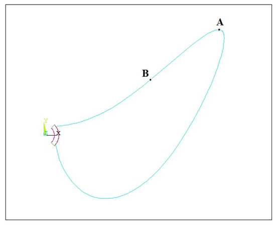
Figure 4.
Definition of design variables A and B of the submerged blade geometry.
This problem is given by the following:
where: ; ; Hz.
Table 8 presents the optimal solutions achieved by GMPBSA and BSA. The optimization objective minimized propeller volume under a critical frequency constraint (Fadm = 65 Hz). This constraint ensures structural integrity by avoiding resonance. LOBSA effectively explored the design space, achieving slightly superior optimal geometry parameters compared to BSA and GMPBSA.
Table 8.
The optimal solutions for the submerged boat propeller.
Here only 100 iterations were used to reduce computational cost of the FSI simulations, since the value of the case study lies in showing that LOBSA can integrate effectively with FSI simulation tools (MATLAB-ANSYS) and maintain at least as good performance as state-of-the-art methods, while its superiority is more clearly demonstrated in the benchmark and constrained design problems.
LOBSA demonstrated superior performance due to effective hybridization, leveraging both rapid local convergence of LO and global robustness of BSA. Computationally, LOBSA introduced minimal overhead while significantly enhancing search capabilities. Sensitivity analyses indicated robustness to parameter tuning, making it suitable for diverse optimization problems. The successful application to fluid–structure interaction showcases potential applicability across multiphysics engineering domains, including aerospace structures, automotive components, and renewable energy systems.
4. Conclusions
This study introduces LOBSA, a novel hybrid evolutionary optimization algorithm combining the strengths of the Backtracking Search Algorithm (BSA) and the Lemurs Optimizer (LO). The hybridization strategically leverages the efficient global search capabilities of BSA and the effective local exploitation characteristics of LO, successfully addressing the balance between exploration and exploitation—a common limitation in conventional optimization algorithms.
Comprehensive validation using a diverse suite of 23 benchmark functions from CEC 2013 highlights LOBSA’s exceptional performance. Statistically significant improvements were demonstrated, with LOBSA consistently achieving superior accuracy and convergence speed compared to standard BSA and other state-of-the-art variants. Practical applicability was further validated through challenging engineering design problems. For the constrained pressure vessel optimization, LOBSA provided the most cost-effective solution among tested algorithms. The successful integration of LOBSA with MATLAB 18.0 and ANSYS 22.0 for optimizing a realistic fluid–structure interaction problem involving a submerged boat propeller further underscores its robustness and suitability for multiphysics applications.
Overall, LOBSA represents a substantial advancement in evolutionary optimization methods, exhibiting versatility, efficiency, and enhanced performance. Its demonstrated capability to solve complex optimization scenarios makes it highly suitable for broader engineering applications in aerospace, mechanical, marine, automotive, and renewable energy fields.
Future work includes extending LOBSA to multi-objective and higher-dimensional optimization problems, conducting more detailed sensitivity analyses, and applying the framework to additional real-world industrial multiphysics problems with a maximum number of iterations to acknowledge its potential limitations obtaining highly improved objective functions. This opens promising avenues for developing efficient, reliable, and practical optimization tools for engineering and scientific communities.
Author Contributions
Conceptualization, K.M.D., A.T.Z. and R.E.M.; Methodology, Validation and Writing—original draft preparation, K.M.D. and A.T.Z.; Software, Formal analysis and Writing—review and editing, R.E.M.; Supervision and Project administration, R.E. All authors have read and agreed to the published version of the manuscript.
Funding
This research received no external funding.
Data Availability Statement
The data presented in this study are available on request from the corresponding author due to privacy of the collaboration.
Conflicts of Interest
The authors declare no conflicts of interest.
Correction Statement
This article has been republished with a minor correction to the Data Availability Statement. This change does not affect the scientific content of the article.
References
- Holland, J.H. Adaptation in Natural and Artificial Systems: An Introductory Analysis with Applications to Biology, Control, and Artificial Intelligence; U Michigan Press: Ann Arbor, MI, USA, 1975. [Google Scholar]
- Kirkpatrick, S.; Gelatt, C.D.; Vecchi, M.P. Optimization by Simulated Annealing. Science 1983, 220, 671–680. [Google Scholar] [CrossRef] [PubMed]
- Kennedy, J.; Eberhart, R. Particle swarm optimization. In Proceedings of the ICNN’95—International Conference on Neural Networks, Perth, WA, Australia, 27 November–1 December 1995; Volume 4, pp. 1942–1948. [Google Scholar] [CrossRef]
- D’Angelo, G.; Della-Morte, D.; Pastore, D.; Donadel, G.; De Stefano, A.; Palmieri, F. Identifying patterns in multiple biomarkers to diagnose diabetic foot using an explainable genetic programming-based approach. Future Gener. Comput. Syst. 2023, 140, 138–150. [Google Scholar] [CrossRef]
- D’Angelo, G.; Palmieri, F.; Robustelli, A. Artificial neural networks for resources optimization in energetic environment. Soft Comput. 2022, 26, 1779–1792. [Google Scholar] [CrossRef]
- Wolpert, D.; Macready, W. No free lunch theorems for optimization. IEEE Trans. Evol. Comput. 1997, 1, 67–82. [Google Scholar] [CrossRef]
- Liu, F.B. Inverse estimation of wall heat flux by using particle swarm optimization algorithm with Gaussian mutation. Int. J. Therm. Sci. 2012, 54, 62–69. [Google Scholar] [CrossRef]
- Tizhoosh, H. Opposition-Based Learning: A New Scheme for Machine Intelligence. In Proceedings of the International Conference on Computational Intelligence for Modelling, Control and Automation and International Conference on Intelligent Agents, Web Technologies and Internet Commerce (CIMCA-IAWTIC’06), Vienna, Austria, 28–30 November 2005; Volume 1, pp. 695–701. [Google Scholar] [CrossRef]
- Kaplan, J. Chaotic behavior of multidimensional difference equations. In Springer Lecture, Notes in Mathematics; Springer: Berlin/Heidelberg, Germany, 1979; Volume 730, pp. 204–227. [Google Scholar] [CrossRef]
- Feynman, R.P. Quantum mechanical computers. Found. Phys. 1986, 16, 507–531. [Google Scholar] [CrossRef]
- Viswanathan, G.M.; Afanasyev, V.; Buldyrev, S.V.; Murphy, E.J.; Prince, P.A.; Stanley, H.E. Lévy flight search patterns of wandering albatrosses. Nature 1996, 381, 413–415. [Google Scholar] [CrossRef]
- Civicioglu, P. Backtracking Search Optimization Algorithm for numerical optimization problems. Appl. Math. Comput. 2013, 219, 8121–8144. [Google Scholar] [CrossRef]
- ElMaani, R.; Radi, B.; Hami, A.E. Numerical Study and Optimization-Based Sensitivity Analysis of a Vertical-Axis Wind Turbine. Energies 2024, 17, 6300. [Google Scholar] [CrossRef]
- Abasi, A.; Makhadmeh, S.; Al-Betar, M.; Alomari, O.; Awadallah, M.; Alyasseri, Z.; Doush, I.; Elnagar, A.; Alkhammash, E.H.; Hadjouni, M. Lemurs Optimizer: A New Metaheuristic Algorithm for Global Optimization. Appl. Sci. 2022, 12, 10057. [Google Scholar] [CrossRef]
- Liang, J.C.; Qu, B.; Suganthan, P.N.; Hernández-Díaz, A.G. Problem Definitions and Evaluation Criteria for the CEC 2013 Special Session on Real-Parameter Optimization. 2013. Available online: https://www.researchgate.net/publication/256995189 (accessed on 24 August 2025).
- Mirjalili, S.; Mirjalili, S.M.; Lewis, A. Grey Wolf Optimizer. Adv. Eng. Softw. 2014, 69, 46–61. [Google Scholar] [CrossRef]
- Mirjalili, S. SCA: A Sine Cosine Algorithm for solving optimization problems. Knowl.-Based Syst. 2016, 96, 120–133. [Google Scholar] [CrossRef]
- Askarzadeh, A. A novel metaheuristic method for solving constrained engineering optimization problems: Crow search algorithm. Comput. Struct. 2016, 169, 1–12. [Google Scholar] [CrossRef]
- Backtracking search algorithm driven by generalized mean position for numerical and industrial engineering problems. Artif. Intell. Rev. 2023, 56, 11985–12031. [CrossRef]
- Mirjalili, S. Moth-flame optimization algorithm: A novel nature-inspired heuristic paradigm. Knowl.-Based Syst. 2015, 89, 228–249. [Google Scholar] [CrossRef]
- Devic, C.; Sigrist, J.; Lainé, C.; Baneat, P. Etude modale numérique et expérimentale d’une hélice marine. In Proceedings of the Septième Colloque National en Calcul des Structures, Giens, France, 15–20 May 2005; Volume 1, pp. 277–282. [Google Scholar]
Disclaimer/Publisher’s Note: The statements, opinions and data contained in all publications are solely those of the individual author(s) and contributor(s) and not of MDPI and/or the editor(s). MDPI and/or the editor(s) disclaim responsibility for any injury to people or property resulting from any ideas, methods, instructions or products referred to in the content. |
© 2025 by the authors. Licensee MDPI, Basel, Switzerland. This article is an open access article distributed under the terms and conditions of the Creative Commons Attribution (CC BY) license (https://creativecommons.org/licenses/by/4.0/).