Abstract
Range height indicator (RHI) scans are performed routinely by the long-range Doppler Light Detection and Ranging (LIDAR) systems at the Hong Kong International Airport (HKIA). This paper presents some novel observations of the airflow in the airport region by RHI scans that have not been reported in the literature in the past—namely, areas of reverse flow and vortex shedding in east to southeasterly winds; severe windshear in the easterly; a converging southerly flow; a descending northeasterly jet; and the undercutting of the southwesterly flow by sea breeze. Many of these flow features are associated with low-level windshear, supported by pilot windshear reports, and thus their observations have practical applications. The technical feasibility of forecasting these airflow features is also studied in this paper, and it is found that large eddy simulations based on a mesoscale meteorology model manage to capture these wind features most of the time, but the simulated headwind change is generally slightly smaller than observed. The results in this paper have application value for windshear alerting and forecasting for an airport situated in an area of complex terrain, and they should be of interest for further studies of mountain meteorology.
1. Introduction
Doppler Light Detection and Ranging (LIDAR) systems are essential tools in monitoring terrain-induced and sea breeze-related windshear and turbulence at the Hong Kong International Airport (HKIA). Based on pilot reports of windshear and turbulence, about 90% of these events occur in clear air conditions. The Hong Kong Observatory (HKO) introduced LIDARs for windshear alerting in 2002. Over the years, a number of scanning strategies in LIDARs have been used operationally for windshear and turbulence detection, including plan position indicator (PPI) scans and glide path scans [1], specifically used to detect abrupt headwind changes along the glide slopes.
With the opening of the third runway at HKIA in November 2024, each runway of the airport was equipped with at least one long-range Doppler LIDAR, covering up to and sometimes beyond three nautical miles from the runway end. With the deployment of a dedicated LIDAR for each runway, there is room for the incorporation of additional scanning strategies for the LIDAR while ensuring frequently updated PPI and glide scans to monitor the overall wind pattern and operational windshear detection, respectively. In early 2025, range height indicator (RHI) scans were incorporated into the scanning patterns of two long-range LIDARs, namely the third runway (north runway) LIDAR located to the south of this runway (HKG3S LIDAR) and the second runway (middle runway) LIDAR (HKG2 LIDAR). The RHI scans have been running for several months since then, collecting some new information about the airflow at HKIA, especially related to the terrain effect or in association with sea breeze. Although they are mainly used for the purpose of monitoring the airflow, their data may have potential to supplement the existing glide path scans for windshear detection.
Airflows in the boundary layer are often studied by Eulerian and Lagrangian turbulence simulation methods in large eddy simulation (LES). The Eulerian method focuses on properties in a fixed reference frame, while the Lagrangian method focuses on reference frame that moves with the flow [2]. These models are applied in computational experiments simulating idealized turbulent [3] or neutral [4] boundary layer flows and pollutant dispersion [5] but are also widely used in weather and climate prediction [6,7,8]. LES is applied for the high-resolution simulation of local wind effects under complex terrain in real-life [9] or for specific local features like foehn-cold pool interaction [10]. In the context of aviation meteorology, LES has also been applied to simulate terrain-induced turbulence in Norway [11] and low-level windshear over Hong Kong [12].
This paper documents, for the first time, a number of novel flow features at HKIA as observed by RHI scans and some PPI scans (namely, a vortex shedding event from a mountain of Lantau Island that has not been observed before). If available, flight data are analyzed to depict the windshear features. The possibility of forecasting such airflow features is also studied by performing a numerical weather prediction (NWP) model simulation down to a spatial resolution of 40 m in the airport area using LES mode. The results in this paper could be useful for reference in aviation weather forecasting, especially for those working at airports with complex terrain, as well as studies of mountain meteorology.
2. Long-Range LIDARs
The long-range LIDARs at HKIA have a measurement range of 10–16 km generally, depending on the weather conditions. The spatial resolution in the radial direction is about 100 m, and it takes a couple of minutes to complete a cycle of PPI scans, as well as a few seconds to complete a glide path scan.
For RHI scans, the HKG3S LIDAR performs one scan at the azimuth angle of 255 degrees, namely for the arrival runway corridor to the west of the north runway (07LA). The HKG2 LIDAR performs three RHI scans, namely at an azimuth angle of 258 degrees (arrival runway corridor to the west of the center runway, 07CA), an azimuth angle of 95 degrees (arrival runway corridor to the east of the center runway, 25CA), and an azimuth angle of 164 degrees (perpendicular to the runway orientation, cutting the major valley of Lantau Island to the south of the airport). The basic specifications of the LIDARs in this study are given in Table 1.

Table 1.
Specifications of HKG1, HKG2, and HKG3S LIDARs.
3. NWP Setup
The Regional Atmospheric Modelling System (RAMS) version 6.3 is used in this study. It is nested with the hourly re-analysis of the European Centre of Medium-Range Weather Forecasts (ECMWF) and has five nesting instances, namely with a spatial resolution of 25 km, 5 km, 1 km, 200 m, and 40 m.
A turbulence parameterization scheme is crucial for the successful simulation of the airflow features. In the three innermost domains, the Deardorff (1980) scheme [13] has been adopted. This scheme is found to provide quality results with a wide range of applications using LES mode, as discussed, for instance, in Gibbs and Fedorovich [14].
4. Case 1: East to Southeasterly Winds
Windshear/turbulence associated with east to southeasterly winds is common at HKIA in spring time. One such case occurred on 26 to 27 April 2025. In this episode, there were 6 pilot reports of encountering low-level windshear, namely, 1051 UTC and 1121 UTC of 26 April at 07LA, 1937, 1956 and 2042 UTC of 26 April at 07CA, and 0101 UTC of 27 April at 07RA (arriving at the south runway of HKIA from the west). The windshear encountering heights, if available, were reported to be 100 to 400 feet. The windshear was mostly headwind gain, with magnitudes of 15 to 25 knots.
The LIDAR observations at about the time of the 07CA windshear report are shown in Figure 1. From the PPI scan (center of the upper panel), east to southeasterly winds prevailed at the airport, and tiny areas of reverse flow (in green) appeared to the west of the airport in association with the wake of the mountains on Lantau Island. Such reverse flow areas travel across all runway corridors to the west of the airport, and significant windshear has been identified in the arrival runway corridors (07LA, 07CA, and 07RA) by the glide path scans (highlighted in blue at the left-hand side of the figure in the upper panel).
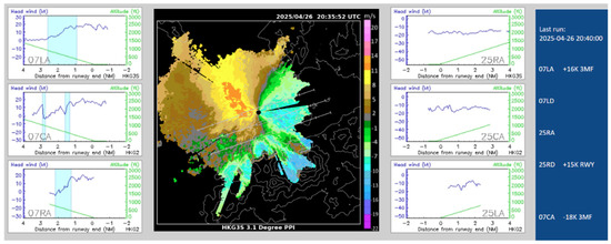
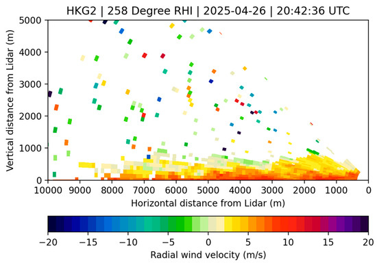
Figure 1.
PPI scan and headwind profiles from the LIDAR on 26 April 2025 (upper panel) and a sample RHI scan (lower panel).
A sample RHI scan by the HKG2 LIDAR at an azimuth angle of 258 degrees is shown in the lower panel of Figure 1. An outbound flow is apparent in the first few hundred meters above ground/sea level in association with the prevailing easterly. This is consistent with the weather buoy observation of an easterly flow near the sea surface. However, slightly higher up, there could be areas of reverse flow (inbound flow, colored green), and waves could be identified at the interface between the outbound and inbound flows. The reverse flow is associated with the mountain wake of Lantau Island.
This pattern persists for many hours and appears at the time of the 07RA windshear report as well (Figure 2). From the upper panel of Figure 2, the headwind profile of 07RA shows rapid fluctuations between the runway end (0 nautical miles) and 1 nautical mile away. A sample RHI scan is shown in the lower panel of Figure 2. The outbound flow near the sea surface and the inbound flow higher up are again observed, and, in fact, the inbound flow may appear to be more extensive, covering a horizontal distance of nearly 1000 m (i.e., between 4500 m and 5500 m from the LIDAR). The co-existence of inbound and outbound flows contributed to the occurrence of low-level windshear encountered by the pilots.
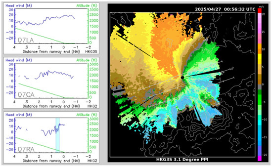

Figure 2.
PPI scan and LIDAR headwind profiles of 27 April 2025 (upper panel) and a sample RHI scan (lower panel).
A sample set of flight data with a pilot windshear report is shown in Figure 3. Because of the terrain disruption of the airflow, multiple occurrences of significant headwind changes could be identified (highlighted in grey), as seen in the upper panel of Figure 3. The headwind changes had a magnitude of around 15 knots and could have been headwind gain or headwind loss. The flight data have been analyzed by the WINDSTURB algorithm [15], as well as the in-house-built software within HKO according to WINDSTRUB and the methodology described in Huang et al. [16]. The results are shown in the lower panel of Figure 3, including the eddy dissipation rate (EDR), as well as the vertical wind. There are discrepancies in the outputs from the two algorithms, but vertical winds have the largest magnitude of around 4 to 6 m/s, and the maximum EDR is in the region of 0.2 to 0.4 m2/3s−1, i.e., moderate turbulence. The mountain wake flow may have created an additional workload for the pilots.
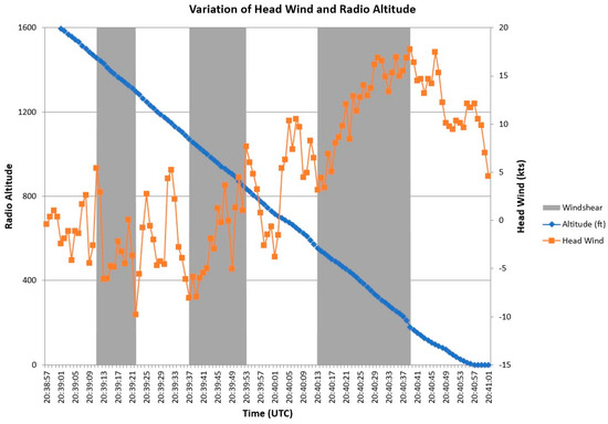
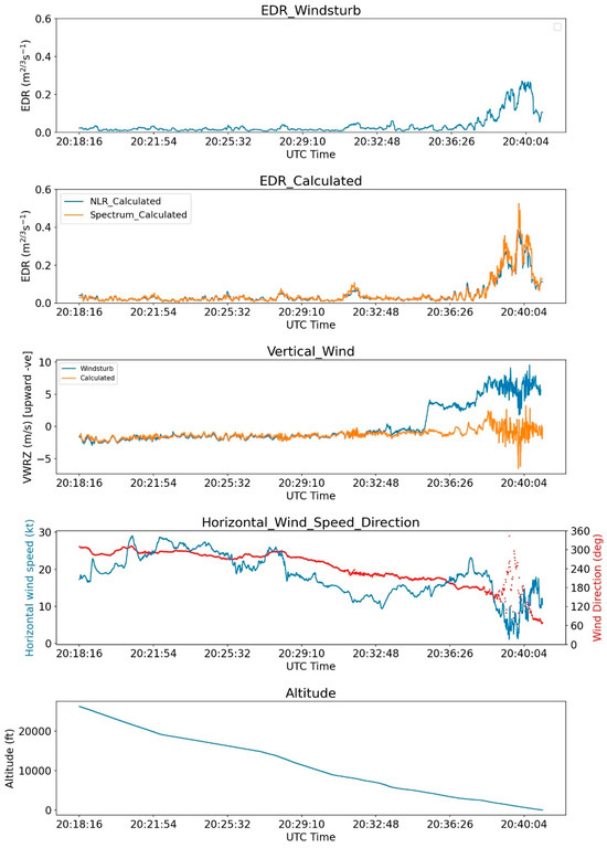
Figure 3.
Headwind profile and windshear for a flight on 26 April 2025 (upper panel) and the detailed analysis (lower panel) with EDR and vertical velocity.
The numerical simulation results are shown in Figure 4. The model was initialized at 12 UTC, 26 April 2025 and it ended at 02 UTC, 27 April 2025. From a sample of the simulated LIDAR velocity imagery (left panel of Figure 4), the reverse flow areas in association with the mountain wake are successfully reproduced. Such areas also appear in the simulated RHI scan velocity imagery (middle panel of Figure 4). The horizontal extent of the inbound flow could reach 1000 m, i.e., between 6500 m and 7500 m from the LIDAR. A sample simulated headwind profile is shown in the right panel of Figure 4. Significant headwind changes are determined by applying the same algorithm used for real LIDAR data [1]. It can be observed that the trend of the simulated headwind profile generally follows the actual headwind profile, with significant headwind loss between 1 to 3 nautical miles from the runway threshold. However, as shown in this case and the subsequent cases, the magnitudes of headwind change in the simulation tended to be smaller than the actual observations, and the simulated fluctuations in the headwind were not as significant as in the actual profile, which is considered to be a limitation of the existing turbulence parameterization scheme.
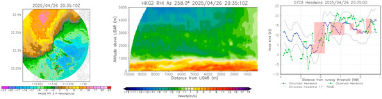
Figure 4.
Simulated PPI scan (left), RHI scan (middle), and headwind profile with windshear (right) for 26 April 2025. For the headwind profile, the blue solid line is the simulated headwind profile and the blue dotted line is the root mean square error (RMSE) range of the profile compared with the observed profile from around 1 h before to 1 h after the time presented; the green line is the observed headwind profile.
The cross-valley RHI scan is inspected as well. A sample observation is shown in the upper panel of Figure 5, and the corresponding simulation is shown in the lower panel of the same figure. The cross-valley inbound flows are very similar in both the observation and simulation. Wave patterns are identified, with strong inbound flows reaching sea level at about 6000–7000 m as well as 2000–3000 m from the LIDAR. Given the simulated PPIs, RHIs, and glide path scans as compared with the actual observations, the NWP model appears to have skills in capturing the main features of the terrain-disrupted airflows.
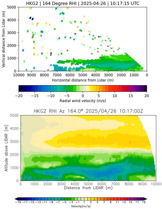
Figure 5.
Actual RHI scan at azimuth angle of 164 degrees (upper) and simulated result (lower).
5. Case 2: Arrival of Easterly and Vortex Shedding During Prevalence of Easterly
At around noon on 2 May 2025, a surge of easterly winds arrived at Hong Kong and gradually extended from the eastern to the western part of the territory. It reached the airport region at around 04 UTC on that day (which was around noon time, with Hong Kong time = UTC + 8 h). The LIDAR observations around that time are given in Figure 6. At that time, southwesterly winds prevailed over the airport, and the easterly winds set in from the east, as shown by the PPI scan image of the LIDAR in the middle of the upper panel of the figure. The interface of the two airmasses resulted in low-level windshear, as shown in the highlighted (blue) regions in the headwind profiles obtained by the LIDAR (on the two sides in the upper panel of the figure). The RHI scan to the east of the airport is shown in the lower panel of Figure 6. The interface of the two airmasses is clearly shown, with the outbound flow associated with the background southwesterly and the inbound flow associated with the easterly. The easterly seems to flow over the background southwesterly, and waves could be identified at the interface between the two airmasses in the vertical cross-section.
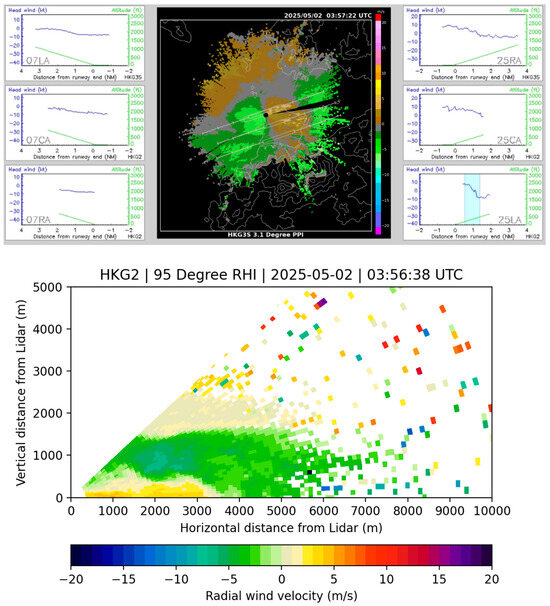
Figure 6.
PPI scan and headwind profiles with windshear (upper panel) and a sample RHI scan (lower panel) for 2 May 2025.
The numerical simulation results are shown in Figure 7. The model was initialized at 00 UTC, 2 May 2025 and run until 15 UTC on that day. At around 04 UTC, the setting in of the easterly is clearly seen in the simulation (upper panel of Figure 7), and the simulated vertical cross displays the interface between the two airmasses (lower panel of the figure). At 0400 UTC, 2 May 2025, an aircraft over the 25RA runway corridor reported encountering windshear of 10 knots with headwind gain at a height of about 400 feet. This is consistent with the actual observations (Figure 6), and the numerical model manages to capture this as well.
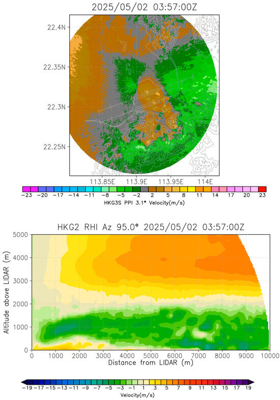
Figure 7.
Simulated PPI scan (upper) and RHI scan (lower) for 2 May 2025.
After the prevalence of the easterly over the airport, vortex shedding appears in the easterly flow, as shown by the LIDAR PPI images. A sequence is shown in Figure 8. Vortex shedding has been reported before at HKIA, including an easterly in spring time [17] and a tropical cyclone situation [18]. The novelty of the present case is that the shedding occurs further to the east, directly downstream of the western side of the U-shaped mountains of Lantau Island. A vertical cross of the shedded vortex is shown in the upper panel of Figure 9. The vortex appears to tilt to the west with the height (green area of inbound flow against the background of outbound easterly flow to the west and to the east of the vortex) and manages to extend to a height of around 1000 m above sea level, which is about the height of the mountains under consideration. As the vortex passes through the runway corridors, low-level windshear occurs, as shown in the blue highlighted regions in the glide path scans in the lower panel of Figure 9. However, on that night, although such windshear alerts had been issued occasionally at different runway corridors to the west of the airport, there were no pilot reports of windshear.
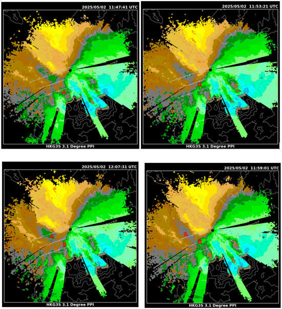
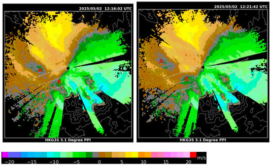
Figure 8.
A sequence of LIDAR PPI scans showing vortex shedding (vortices A and B) on 2 May 2025.
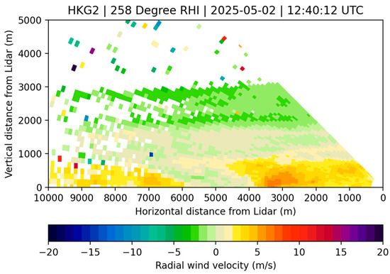
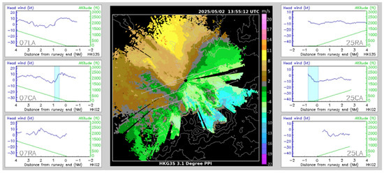
Figure 9.
RHI scan of the LIDAR (upper) and PPI scan with headwind profiles and windshear (lower) for 2 May 2025.
Between 11:30 UTC and 14:00 UTC, 2 May 2025, there were five sheddings of vortices, with the total time of 9000 s. As such, the shedding period is about = 9000 s/5 = 1800 s. According to the review of Atkinson [19], the shedding period could be expressed in terms of the Strouhal number () and the horizontal dimension of the obstacle:
where is the mean background wind speed. Based on the background wind speed profile from King’s Park, is taken to be 6 m/s, is taken to be 4000 m for Lo Fu Tau, and is 0.37, which is close to the range of 0.15 to 0.32 given by Atkinson [19].
Following Vosper [20], vortex shedding would occur for ≤ 0.4, with the Froude number defined by
where is the buoyancy frequency and is the mountain height, which is taken to be 934 m. From the sounding data collected at King’s Park, is about 0.0135 s−1. As a result, is about 0.476, which is only slightly larger than the range given by Vosper [20].
The results of the numerical simulation for shedding are given in Figure 10. The shedding could be captured by the simulation, but the shedding period is different. For the sequence in Figure 10, the shedding period is about 1200 s only. In general, a number of sheddings appear in the simulation, but the shedding periods are mostly around 1000 s. A vertical cross-section of the simulation is shown in the upper panel of Figure 11. The height of the vortex is about 1000 m above sea level, but the structure does not appear to be coherent. In association with such a vortex, low-level windshear has been simulated, as shown in the lower panel of Figure 11. The shape of the headwind profile is generally consistent with that of the observation, but the trough of the headwind shifted to the east for around 0.5–1 nautical miles, likely because of the difference in the shedding period between the observation and simulation, so the phase of the vortex experienced in the simulated headwind profile could differ from the actual situation. Due to being persistently out of phase, the RMSE of the simulated headwind in this case is 6.7 knots, higher than the 5.4 knots in Case 1. The simulated results are considered to indicate mixed success, bearing some similarities with the actual observations of the shedding.
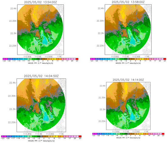
Figure 10.
Simulated sequence of PPI scans showing vortex shedding (vortices A and B) for 2 May 2025.
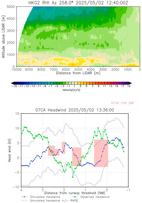
Figure 11.
Simulated RHI scan (upper) and headwind profile with windshear (lower) for 2 May 2025. The meaning of the lines in the headwind profile follows the lower panel of Figure 4.
6. Case 3: Southerly Winds
Moderate to fresh southerly winds prevailed over the airport region on 4 May 2025. The prevailing winds penetrated through three major valleys of the mountainous terrain on Lantau Island to the south of HKIA, namely the gap at the eastern part, center part, and western part of the island. After passing through these gaps, the southerlies converged over the airport island. A snapshot of the Doppler velocity image of the LIDAR is shown in the middle of the upper panel of Figure 12. As a result of the airflow convergence, low-level windshear occurs rather close to the runway ends, as highlighted in blue in the headwind profiles on the two sides of the upper panel of Figure 12. On that day, there were two pilot windshear reports over 07RA, at 0640 UTC and 0702 UTC. Both reported encountering headwind gains of 15 to 20 knots at a height of about 300 feet, at about one nautical mile from the runway end. They had conducted a missed approach because the windshear was very close to the runway end.
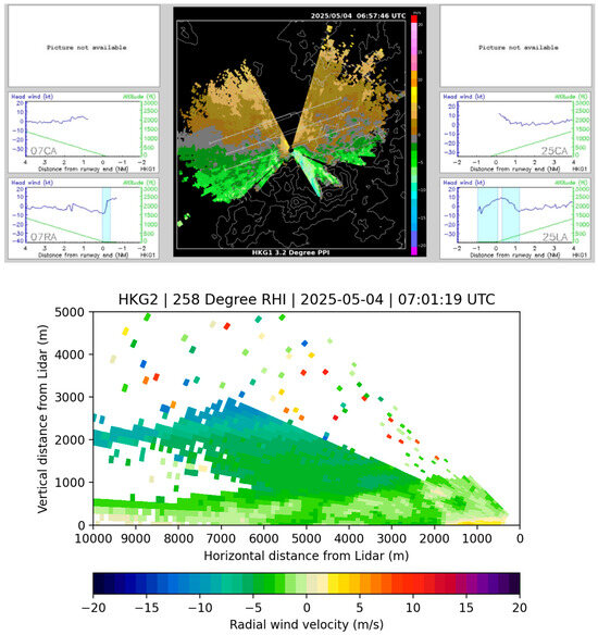
Figure 12.
PPI scan with headwind profiles and windshear (upper) and RHI scan (lower) for 4 May 2025.
A sample RHI scan of the LIDAR is shown in the lower panel of Figure 12. A converging flow is apparent near the runway end (i.e., at about 2000 m to the west of the LIDAR), with the outbound flow (yellow) converging with the inbound flow (green). The two airflows are rather shallow, extending up to several hundred meters above sea level only.
The flight data from one of the flights conducting a missed approach are shown in Figure 13. In the upper panel of the figure, the headwind is shown, with the windshear highlighted in grey. The headwind gain reached around 20 knots and occurred near the touchdown. The wind changes are consistent with the LIDAR observations. The flight data were analyzed in detail using the WINDSTURB algorithm and the HKO in-house algorithm, and the results are shown in the lower panel of Figure 13. In general, the results from the two algorithms are consistent with each other. The EDR reached about 0.4 m2/3s−1, i.e., encountering moderate to severe turbulence. The vertical velocity is in the region of +6 m/s (upward motion) to −2 m/s (downward motion).
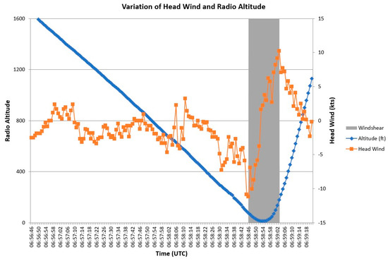
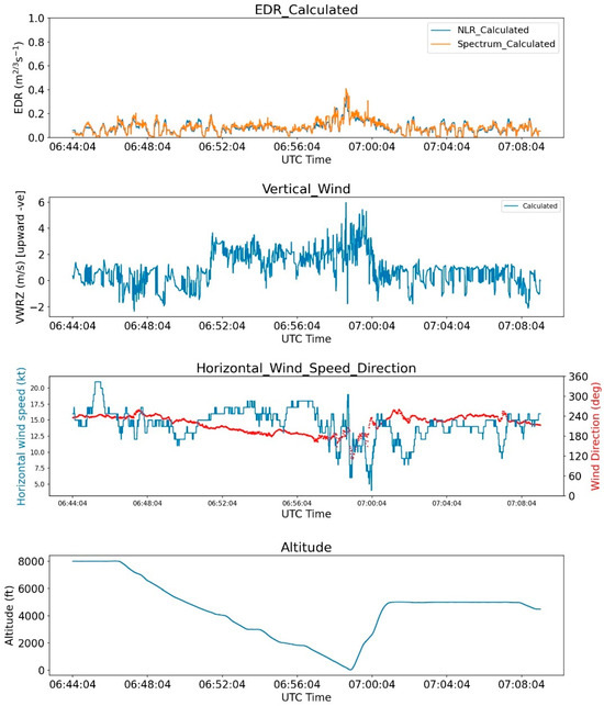
Figure 13.
Headwind profile (upper) and analysis (lower) for data of a flight on 4 May 2025.
A numerical simulation has been conducted, and the model was initialized at 03 UTC of 4 May 2025. A sample of the simulated LIDAR PPI scan is shown in the left panel of Figure 14. The pattern is similar to the actual observations (upper panel of Figure 12). The corresponding simulated RHI scan is shown in the middle panel of Figure 14. The converging flows and their heights are similar to the actual observations (lower panel of Figure 12), although the location of the convergence is located over the western part of the runway instead of being very close to the runway end. The corresponding headwind profile is shown in the right panel of Figure 14. The significant headwind gain was simulated successfully, and the trend of the headwind change matched between both headwind profiles, although the magnitude in the simulated profile was lower than in the actual observation (15-knot headwind gain). The RMSE for the simulated headwind profile is about 5.5 knots for this case.
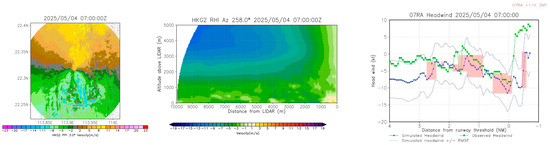
Figure 14.
Simulated PPI (left), RHI (middle), and headwind profile with windshear (right) on 4 May 2025. The meaning of the lines in the headwind profile follows the lower panel of Figure 4.
7. Case 4: Severe Turbulence in East to Southeasterly Flow
In terms of the flow pattern at the airport region, this case is similar to Case 1, i.e., as shown in the PPI scan in the upper panel of Figure 15, together with the associated headwind profiles. The special feature of this case is a pilot windshear report of −40 knots (headwind loss) at a height of 100 feet over 07CA at 2151 UTC, 7 May 2025, leading to a missed approach. This magnitude of headwind loss is not apparent from the headwind profile of the LIDAR, as well as the RHI scan, as shown in the middle panel of Figure 15. From the RHI scan, an outbound easterly flow prevails over the 07CA runway corridor, with a slightly weaker wind above the strong outbound flow, i.e., between 5000 m and 7000 m from the LIDAR. The flight path of the aircraft is overlaid on this RHI scan, and the headwind is derived with the headwind profile shown in the lower panel of Figure 15. As such, apart from the headwind profile obtained from the glide path scans of the LIDAR, the RHI scan data are used for the first time to derive the headwind profile as well. However, there is only a headwind loss of around 15 knots, from around 20 knots to 5 knots. The RHI data also do not show headwind loss up to 40 knots.
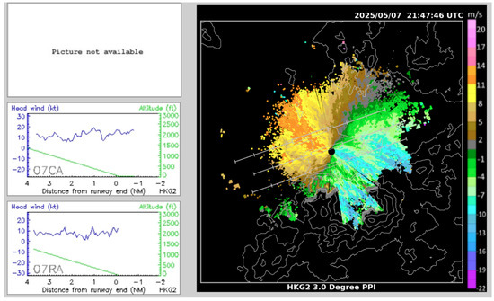
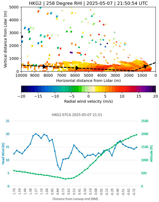
Figure 15.
PPI scan wind headwind profile (upper), RHI scan (middle), and headwind profile derived from RHI scan (lower) for 7 May 2025. The dashed line in the middle figure and the green line in the lower figure are rough traces of the flight.
The flight data are shown in Figure 16. The headwind profile is shown in the upper panel, and the windshear (highlighted in grey) is only about 16 knots of headwind loss. The data are shown in detail in the lower panel of Figure 16, with the EDR reaching about 0.4 m2/3s−1 (moderate to severe turbulence) and vertical wind in the region of +5 m/s (upward motion) and −3 m/s (downward motion). Pilot windshear reports are more subjective, and the estimation of headwind changes is difficult, possibly making reference to the airspeed changes. The severe windshear reported in this case may be related to the rather abrupt loss of headwind near the runway end, together with the occurrence of moderate to severe turbulence.
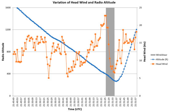
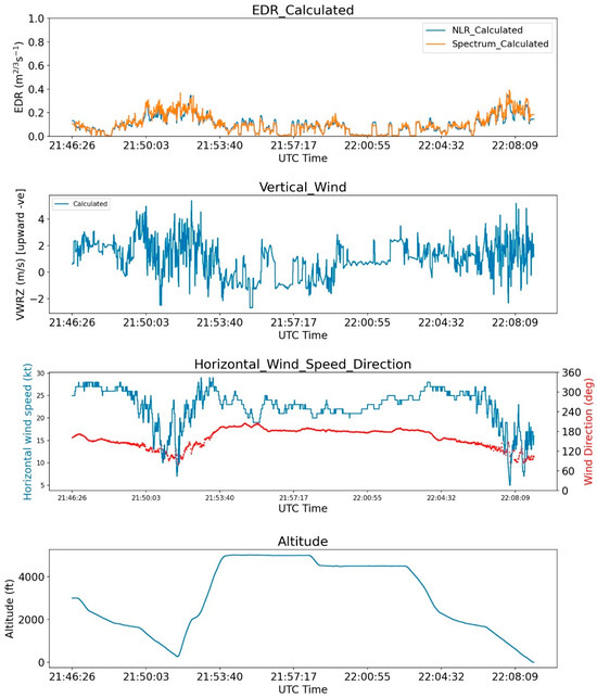
Figure 16.
Headwind profile with windshear (upper) and detailed analysis (lower) for a flight with data on 7 May 2025.
The numerical simulation generally supports the actual observations. It is initialized at 18 UTC. The simulated PPI scan is shown in the upper panel of Figure 17, generally consistent with the actual observations in the upper panel of Figure 15. In the simulated RHI scan in the middle panel of Figure 17, a slightly weaker outbound flow appears at a height of several hundred meters above sea level, between 4000 m and 6000 m from the LIDAR. It is related to the headwind gain and headwind loss in that region, as shown in the simulated headwind profile in the lower panel of Figure 17. The headwind changes have a magnitude of 10 to 15 knots only. This is also the case with the lowest RMSE among the four presented cases, which is only 4.5 knots.
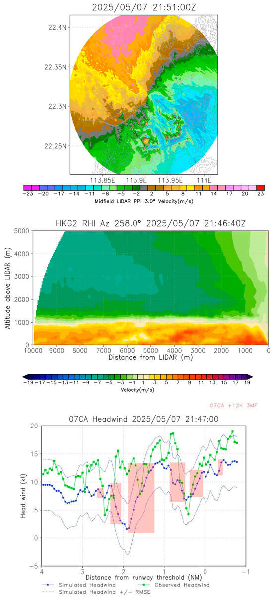
Figure 17.
Simulated PPI (upper), RHI (middle), and headwind profile (lower) for 7 May 2025. The meaning of the lines in the headwind profile follows the lower panel of Figure 4.
8. Case 5: Descending Jet in Northeasterly
It is not common to have strong northeasterly winds in Hong Kong as late as May (late spring), and one such case occurred on 10 May 2025. There are no windshear reports in this case. The LIDAR PPI image is shown in the upper panel of Figure 18. A disturbed flow appears as the background, strong northeasterly winds flow over and past the terrain to the north and northeast of HKIA. In the RHI scan of the LIDAR, at an azimuth angle of 164 degrees, an outbound (background northeasterly) jet first appeared at a height of around 500 m above sea level near the LIDAR and descended to near the ground at a distance of about 6000 m to 7000 m from the LIDAR. This descending has never been observed in Hong Kong before.
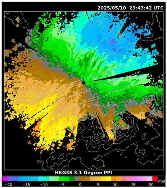
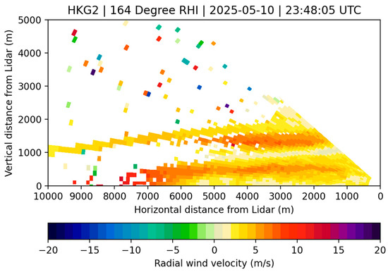
Figure 18.
PPI scan (upper) and RHI with azimuth angle of 164 degrees (lower) for 10 May 2025.
A numerical simulation is performed, initialized at 21 UTC, 10 May 2025. The simulated PPI scan and RHI scan (azimuth angle of 164 degrees) are shown in the upper panel and lower panel, respectively, of Figure 19. In general, the actual observations are successfully reproduced. In particular, the descending emerges well, together with the inbound and outbound flow aloft.
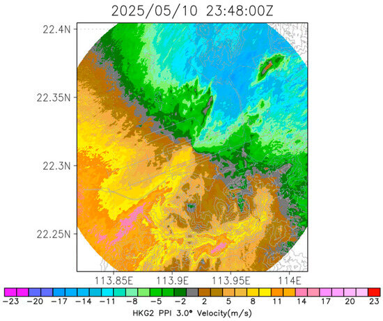
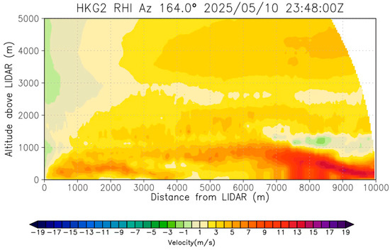
Figure 19.
Simulated PPI scan (upper) and RHI scan (lower) for 10 May 2025.
9. Case 6: Uplifting of Background Flow with Setting in of Sea Breeze
In the late afternoon of 12 May 2025, a southwesterly prevailed over the airport region. With abundant sunshine, easterly sea breeze set in over the eastern part of HKIA. The PPI scan at that time is shown in the upper panel of Figure 20. The convergence between the background southwesterly and the easterly sea breeze could have led to low-level windshear, although there were no pilot reports of windshear for this case. However, from the RHI, it is observed, for the first time, that the setting in of the sea breeze (inbound flow in green) uplifted the background southwesterly (outbound flow in yellow), as shown in the sequence of RHI scans in the lower panel of Figure 20. The lifting is possibly due to the slightly cooler airmass associated with the sea breeze.
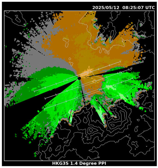
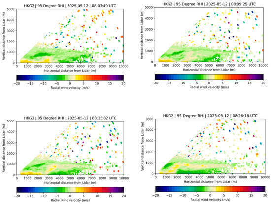
Figure 20.
PPI scan (upper) and sequence of RHI scan at an azimuth angle of 95 degrees (lower) for 12 May 2025.
To simulate the process, the NWP model is initialized at 05 UTC, 12 May 2025. At around 08 UTC, the sea breeze begins to set in from the east in the simulated PPI scan (upper panel of Figure 21). A sequence of simulated RHI scans at an azimuth angle of 95 degrees is shown in the lower panel of Figure 21. The uplifting of the outbound flow is successfully captured in the simulation. Based on the simulation results, a temperature difference is identified between the background southwesterly wind and the easterly sea breeze, which is believed to be related to the uplifting of the outbound flow.
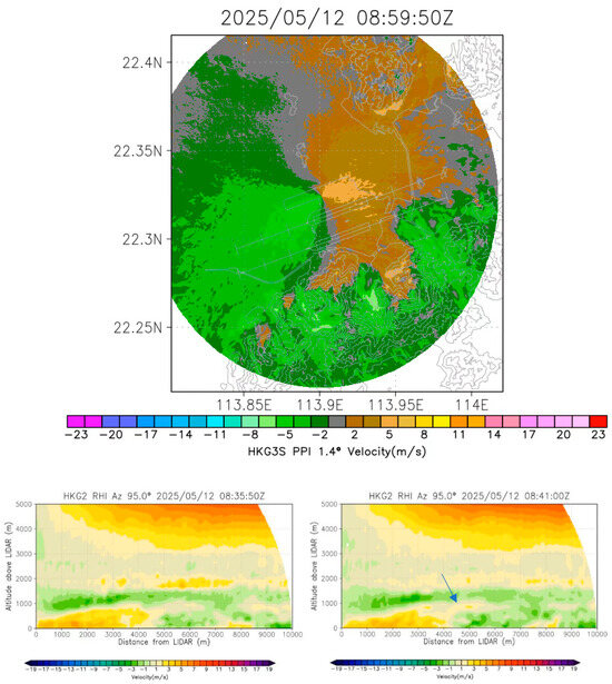
Figure 21.
Simulated PPI image (upper) and simulated sequence of RHI images for an azimuth angle of 95 degrees (lower). The uplifted outbound flow is indicated by a blue arrow.
10. Conclusions
The present paper summarizes a number of novel observations of the vertical structure of the airflow at HKIA from RHI scans of the long-range LIDAR, which could not be identified solely using PPI scans. The cross-sections of vortex shedding behavior over the mountains of Lantau Island, the uplift of the background easterly flow by the sea breeze, and even a change in the jet core height along the RHI scanning direction could be clearly depicted by the scans. When aircraft pass through flow boundaries caused by the terrain, sea breeze, or low-level jets, even if the scale of the boundary is small, low-level windshear could be experienced by the aircraft and impact flight safety. RHI scans are able to portray the detailed vertical structure of the airflow, particularly along the arrival and departure glide paths, and supplement the headwind profiles obtained by traditional LIDAR scans for the monitoring and even notification of low-level windshear. The windshear cases, as shown in the RHI scans, are generally consistent with the pilot reports, although discrepancies have been observed, e.g., for the severe windshear case. This could be related to the subjective nature of pilot windshear reports, but the reports are generally useful for scientific investigations when compared with other observations and measurements [21].
Numerical simulations have been performed to reproduce the airflow features by using the simulated PPI scans, RHI scans, and headwind profiles. The mesoscale meteorological model running in LES mode shows the capability of capturing the main features of the windshear and the pattern of headwind change. The RMSEs of the simulated headwind profiles are generally 5 knots when low-level windshear is a result of synoptic setting, but the error is much larger in the vortex shedding case, in which the simulated and actual vortex shedding periods are different, so the resulting headwind change would be out of phase. For most cases, the magnitude of the headwind change is normally underestimated, likely due to the sensitivity of the model and also the variable nature of turbulent flows. For headwind profiles generated from LIDAR and QAR, the wind speed can vary significantly within a couple of hundreds of meters or a few seconds of time in the air. This means that the actual wind can show even greater variability than the simulated wind field, and the further development of turbulence parameterization schemes may be necessary.
The present paper serves as a reference for other airports located in similarly complex terrain, especially those situated near mountains, which may be affected by terrain-induced turbulence, such as in Norway [11], or those situated over islands, in which the sea breeze effect may play a role in low-level windshear, as at Incheon Airport [22]. By comparing numerical simulations and observations, it is shown that the PPI, RHI, and glide path scans of LIDARs are able to capture many features of the airflow in complex terrain and the changes in headwind profile; these could assist aviation forecasters in the monitoring and even notification of low-level windshear and turbulence from a nowcasting perspective. In this paper, the use of high-resolution NWP with LES mode took about 60 h to generate a 3-h simulation using a desktop computer; the runtime could potentially be reduced significantly by implementing the model on a high-performance computer, producing short-term forecasts in a reasonable time frame. If this is possible, patterns of the expected low-level windshear and turbulence could generally be simulated in real time and could serve as guidance for aviation forecasters. However, with regard to a provisional warning, the magnitude of the windshear may need to be adjusted from the model output based on the forecaster’s experience, the local topography, background forcing, and the nature of the windshear.
Author Contributions
Conceptualization, P.-w.C. and P.C.; methodology, P.-w.C. and P.C.; software, P.C. and K.-k.L.; validation, P.C., M.-l.C. and K.-k.L.; formal analysis, P.-w.C. and M.-l.C.; investigation, P.C. and K.-k.L.; resources, P.-w.C. and P.C.; data curation, M.-l.C. and K.-k.L.; writing—original draft preparation, P.-w.C.; writing—review and editing, M.-l.C.; visualization, M.-l.C. and K.-k.L.; supervision, P.-w.C. and P.C.; project administration, P.-w.C. All authors have read and agreed to the published version of the manuscript.
Funding
This research received no external funding.
Institutional Review Board Statement
Not applicable.
Informed Consent Statement
Not applicable.
Data Availability Statement
The data presented in this study are available on request from the corresponding author.
Acknowledgments
The use of QAR data for scientific purposes was made possible through the kind permission of Cathay Pacific.
Conflicts of Interest
The authors declare no conflict of interest.
References
- Shun, C.M.; Chan, P.W. Applications of an Infrared Doppler Lidar in Detection of Wind Shear. J. Atmos. Ocean. Technol. 2008, 25, 637–655. [Google Scholar] [CrossRef]
- Dosio, A.; Guerau de Arellano, J.V.; Holtslag, A.A.M.; Builtjes, P.J.H. Relating Eulerian and Lagrangian Statistics for the Turbulent Dispersion in the Atmospheric Convective Boundary Layer. J. Atmos. Sci. 2005, 62, 1175–1191. [Google Scholar] [CrossRef]
- Slinn, D.N.; Riley, J.J. A Model for the Simulation of Turbulent Boundary Layers in an Incompressible Stratified Flow. J. Comput. Phys. 1998, 144, 550–602. [Google Scholar] [CrossRef]
- Vasaturo, R.; Kalkman, I.; Blocken, B.; van Wesemael, P.J.V. Large eddy simulation of the neutral atmospheric boundary layer: Performance evaluation of three inflow methods for terrains with different roughness. J. Wind Eng. Ind. Aerodyn. 2018, 173, 247–261. [Google Scholar] [CrossRef]
- Lin, C.; Ooka, R.; Jia, H.; Parente, A.; Kikumoto, H. Eulerian RANS simulation of pollutant dispersion in atmospheric boundary layer considering anisotropic and near-source diffusivity behavior. J. Wind Eng. Ind. Aerodyn. 2025, 258, 106036. [Google Scholar] [CrossRef]
- Stoll, R.; Gibbs, J.A.; Salesky, S.T.; Anderson, W.; Calaf, M. Large-Eddy Simulation of the Atmospheric Boundary Layer. Bound. -Layer Meteorol. 2020, 177, 541–581. [Google Scholar] [CrossRef]
- Atlas, R.L.; Bretherton, C.S.; Blossey, P.N.; Gettelman, A.; Bardeen, C.; Lin, P.; Ming, Y. How Well Do Large-Eddy Simulations and Global Climate Models Represent Observed Boundary Layer Structures and Low Clouds Over the Summertime Southern Ocean? J. Adv. Model. Earth Syst. 2020, 12, e2020MS002205. [Google Scholar] [CrossRef]
- Schalkwijk, J.; Jonker, H.J.J.; Siebesma, A.P.; van Meijgaard, E. Weather Forecasting Using GPU-Based Large-Eddy Simulations. Bull. Amer. Meteor. Soc. 2015, 96, 715–723. [Google Scholar] [CrossRef]
- Rohanizadegan, M.; Petrone, R.M.; Pomeroy, J.W.; Kosovic, B.; Muñoz-Esparza, D.; Helgason, W.D. High-Resolution Large-Eddy simulations of flow in the complex terrain of the Canadian Rockies. Earth Space Sci. 2023, 10, e2023EA003166. [Google Scholar] [CrossRef]
- Umek, L.; Gohm, A.; Haid, M.; Ward, H.C.; Rotach, M.W. Influence of grid resolution of large-eddy simulations on foehn-cold pool interaction. Q. J. R. Meteorol. Soc. 2022, 148, 1840–1863. [Google Scholar] [CrossRef] [PubMed]
- Wang, S.; De Roo, F.; Thobois, L.; Reuder, J. Characterization of Terrain-Induced Turbulence by Large-Eddy Simulation for Air Safety Considerations in Airport Siting. Atmosphere 2022, 13, 952. [Google Scholar] [CrossRef]
- Chan, P.W.; Lai, K.K.; Li, Q.S. High-resolution (40 m) simulation of a severe case of low-level windshear at the Hong Kong International Airport—Comparison with observations and skills in windshear alerting. Meteorol. Appl. 2021, 28, e2020. [Google Scholar] [CrossRef]
- Deardorff, J.W. Stratocumulus-capped mixed layers derived from a three-dimensional model. Bound. Layer Meteorol. 1980, 18, 495–527. [Google Scholar] [CrossRef]
- Gibbs, J.A.; Fedorovich, E. Sensitivity of turbulence statistics in the lower portion of a numerically simulated stable boundary layer to parameters of the Deardorff subgrid turbulence model. Q. J. R. Meteorol. Soc. 2016, 142, 2205–2213. [Google Scholar] [CrossRef]
- Haverdings, H.; Chan, P.W. Quick access recorder data analysis software for windshear and turbulence studies. J. Aircr. 2010, 47, 1443–1447. [Google Scholar] [CrossRef]
- Huang, R.; Sun, H.; Wu, C.; Wang, C.; Lu, B. Estimating Eddy Dissipation Rate with QAR Flight Big Data. Appl. Sci. 2019, 9, 5192. [Google Scholar] [CrossRef]
- Chan, P.W. Observation and numerical simulation of an event of vortex/wave shedding from a mountain near the Hong Kong International Airport. Meteorol. Appl. 2012, 19, 371–384. [Google Scholar] [CrossRef]
- Chan, P.W. Observation and numerical simulation of vortex/wave shedding for terrain-disrupted airflow at Hong Kong International Airport during Typhoon Nesat in 2011. Meteorol. Appl. 2014, 21, 512–520. [Google Scholar] [CrossRef]
- Atkinson, B.W. Meso-Scale Atmospheric Circulations; Academic Press: London, UK, 1981; 495p. [Google Scholar]
- Vosper, S.B. Three-dimensional numerical simulations of strongly stratified flow past conical orography. J. Atmos. Sci. 2000, 57, 3716–3739. [Google Scholar] [CrossRef]
- Schwartz, B. The quantitative use of PIREPs in developing aviation weather guidance products. Weather Forecast. 1996, 11, 372–384. [Google Scholar] [CrossRef]
- Lee, Y.H.; Min, K.H. Analysis of Low-Level Winds at the Incheon International Airport. AGU24. 2024. Available online: https://agu.confex.com/agu/agu24/meetingapp.cgi/Paper/1583525 (accessed on 20 August 2025).
Disclaimer/Publisher’s Note: The statements, opinions and data contained in all publications are solely those of the individual author(s) and contributor(s) and not of MDPI and/or the editor(s). MDPI and/or the editor(s) disclaim responsibility for any injury to people or property resulting from any ideas, methods, instructions or products referred to in the content. |
© 2025 by the authors. Licensee MDPI, Basel, Switzerland. This article is an open access article distributed under the terms and conditions of the Creative Commons Attribution (CC BY) license (https://creativecommons.org/licenses/by/4.0/).