Design of Pixelated Wideband Metasurface Absorber Using Transfer Learning and Generative Adversarial Networks

Abstract

In this paper, a wideband metasurface absorber is proposed by utilizing transfer learning and a conditional deep convolutional generative adversarial network (CDCGAN). This approach involves introducing a forward prediction neural network to predict the spectral curve of a metasurface absorber, as well as a generative adversarial network for the inverse design of a metasurface absorber. After comparing different pre-trained models, a transfer learning network (TLN) based on GoogleNet-InceptionV3 is incorporated into the design process to reduce the amount of training data required. Based on the pixelated metasurface with a common effect of metallic pixels and resistive film pixels, a broadband electromagnetic absorber was designed through the CDCGAN model. For the application target of the C-band, a pixelated broadband metasurface Absorber I has been designed, which can achieve an absorption effect of less than −8 dB in the range of 6.5–8 GHz, and the absorption performance reaches less than −15 dB near the resonant frequency point of 7 GHz. Further lightweight optimization design was carried out, and the metasurface Absorber II was designed for application in the X-band, which has an absorption bandwidth below −8 dB at 9–12 GHz. The reflectivity curve measured by the experiment is in good agreement with that of the simulation result. Of note, our methodology aims to reversely engineer suitable absorbing structures based on customer-defined spectrums, which may bear some significance to the rapid design of broadband metasurface absorbers.

1. Introduction

Metasurfaces are artificially layered materials with a thickness smaller than the wavelength of electromagnetic radiation, and they are typically arranged in a periodic fashion [1]. The sub-wavelength structures enable them to effectively manipulate various properties of electromagnetic waves, including the polarization [2,3], amplitude [4,5], phase [6], and polarization mode [7,8]. In parallel, metasurfaces can exhibit fascinating characteristics such as negative refraction [9,10], superlensing, zero magnetic permeability, and invisibility cloaking [11,12]. Recent advances in resistive film integration have further enhanced metasurface absorbers by combining ohmic loss and impedance matching for broadband performance. For instance, Zhou et al. [13] designed a screen-printed resistive film-based frequency-selective rasorber with dual absorption bandsand low insertion loss. Ghadimi et al. achieved a 175% fractional bandwidth using pixelated resistive films optimized via a binary particle swarm algorithm [14], while Li et al. proposed a circuit pattern mapping method to correlate resistive film geometries with impedance dispersion for wideband absorption [15]. Despite these successes, traditional design approaches remain computationally intensive and rely heavily on iterative simulations. Under most circumstances, the design process requires researchers to have accumulated knowledge and relevant design experiences, enabling them to effectively resolve various issues and continually optimize the designed structure [16,17]. Generally, an entire design procedure includes pattern design, modeling and simulation, comparing the simulation results with the expected performance, and then continuously optimizing until the target effect is achieved. This procedure is widely adapted in relevant works, such as the design and optimization of multifunctional metasurfaces proposed in recent years [18,19,20]. The whole process is very time consuming and poses a great challenge to both computer and engaged professionals.

In recent years, machine learning, as an emerging interdisciplinary subject, has played a significant role in many engineering fields. The team led by Tiejun Cui proposed the concepts of “encoding metamaterials” and “digital metamaterials” [21], making it easier to incorporate machine learning into the design of metasurfaces. Based on the microscope meta-atoms, Zhang et al. proposed a machine learning method that linked deep learning and BPSO for searching the optimal reflection phases of two-unit cells for the desired target [22]. The system can realize automatic designs from the desired reflection phase performance to the target element patterns. Wei Ma et al. reported a deep learning-based model, comprising two bidirectional neural networks assembled by a partial stacking strategy, to automatically design and optimize three-dimensional chiral metamaterials with strong chiroptical responses at predesignated wavelengths [23].

Integrating deep learning into solving electromagnetic metasurface problems releases researchers from complex modeling and solving processes, thus enabling them to focus on learning the relationship between the structure of electromagnetic metasurfaces and their corresponding electromagnetic responses [24,25]. Basically, based on different inputs and outputs, there are two categories of metasurface design problems [26,27]. The first category takes the structure pattern or parameters of the metasurface as input and generates the corresponding frequency spectrum curve as output. This category is usually referred as a forward prediction network, which functions similarly to traditional electromagnetic simulation software but eliminates the need for complex modeling processes. The other type is the inverse design, which takes the target frequency spectrum curve as input and produces the metasurface structure parameters or patterns as output, aiming to optimize the metasurface design process by generating the most suitable metasurface structure to achieve the desired electromagnetic response. For example, in 2018, Liu et al. trained a generative adversarial network (GAN) by using a dataset composed of randomly shaped images [28]. The network architecture consisted of three parts: a simulator, a generator, and a critic. This approach effectively discovered and optimized unit patterns of metasurfaces to respond to user-defined spectra at the input end. In the same year, Jiang et al. introduced a GAN-based method for designing freeform diffractive elements [29]. They created a dataset containing diffraction patterns and then trained it using the GAN algorithm, where the two parts of the GAN network competed against each other.

Deep neural networks have been introduced in the field of meta-material as a powerful way of obtaining the nonlinear mapping between the topology and composition of arbitrary structures and their associated functional properties [30]. Up to date, plenty of research has been carried out to design metasurfaces by means of deep learning; however, they are mainly concentrating on phase predictions [31]. The normalized operation of the reflected phase in the range of 1° to 360° is used to establish a one-to-one correspondence between the phase and the meta-atom, which is actually a classification problem. However, predicting the reflectance spectrum is more complex than phase-pattern mapping, because the continuous spectrum is a one-to-many mapping of the metasurface at different frequency points. Another hinderance is that, as a data-hungry method, deep learning can only work well if fed with massive data [27]. More often than not, to achieve a high enough accuracy, researchers tend to train the DLN on the base of a huge dataset, which, from another perspective, requires more time cost and computer resources, since collecting a large amount of data is slow and expensive for numerical simulations. Nevertheless, in the field of engineering applications, the meta-atoms arrayed on the metasurfaces have many distribution modes, making it barely possible to collect adequate datasets that are necessary for the DLN.

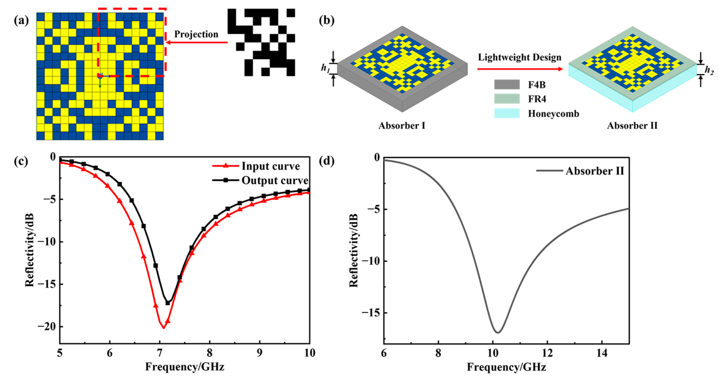
Here, a transfer learning network (TLN) is built to predict the spectrum curve of an input metasurface pattern. By leveraging pre-trained models for metasurface design, we can exploit their learned features and employ suitable fine-tuning techniques to adapt the model to the specific task at hand. This approach can enhance training accuracy, expedite model convergence, and enable faster attainment of exceptional design results. On this basis, we adopt a conditional deep convolutional generative adversarial network (CDCGAN) to accomplish designing metasurfaces in reverse. In the inverse design, we input the desired reflectance spectrum as a condition into the network model, from which the already trained CDCGAN outputs the corresponding metasurface pattern. Simulations and experiments verify the accuracy and high efficiency of our model. Introducing transfer learning to build the network architecture has some enlightening significance to guide the design of a wideband metasurface absorber.

2. Materials and Methods

2.1. Preparation of Dataset

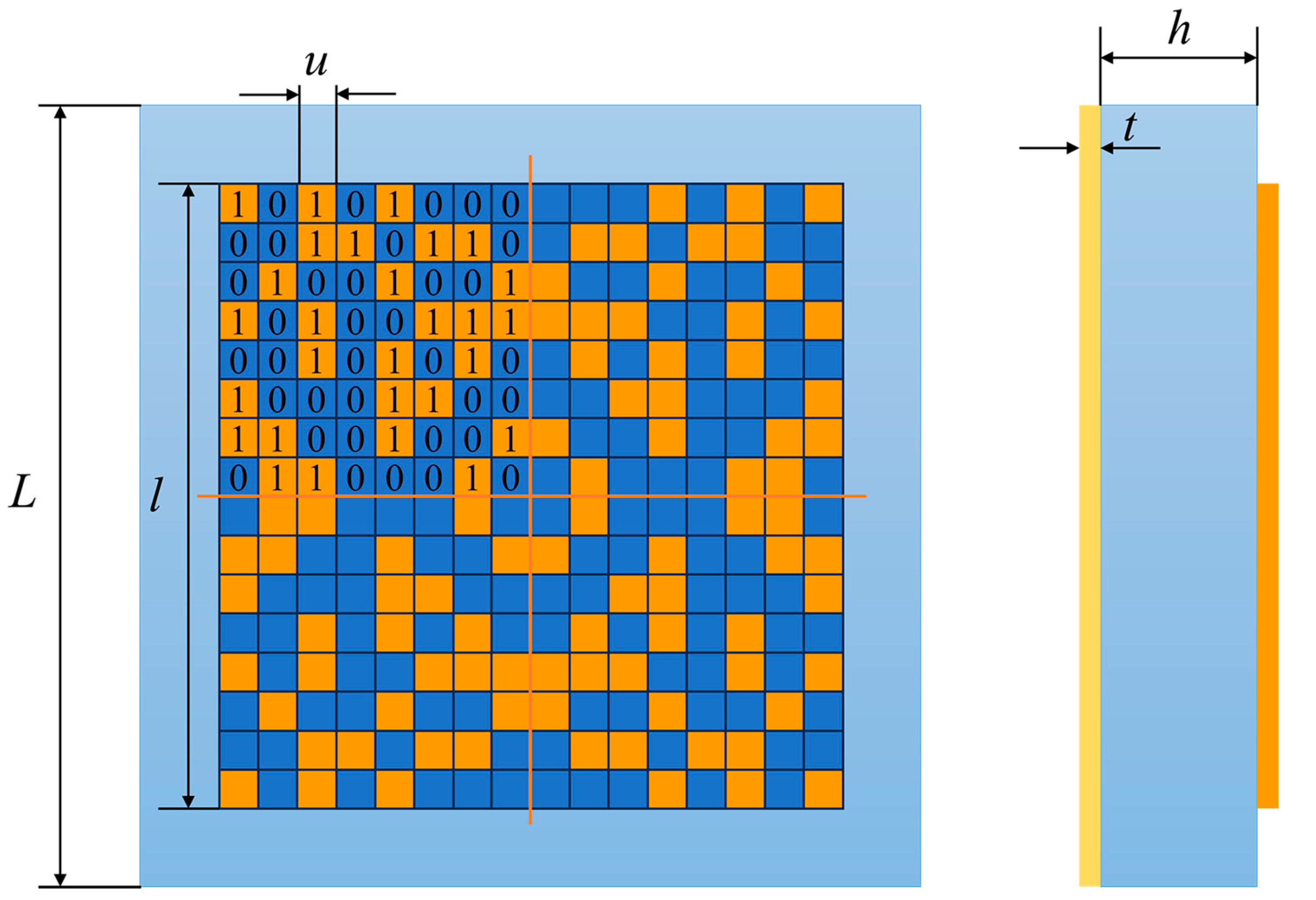
During the data collection procedure for the meta-atom dataset in our study, we adopted the High Frequency Structure Simulator (HFSS) to collect the S-parameter performance curves of metasurface absorbers with different pixelated codes and the comparison relationship of their topological patterns. Figure 1 depicts the structure of a metasurface and the coding of a meta-atom pattern. On the left is the top view, where the top layer represents the encoding sequence of the meta-atom pattern, and this figure just shows one possible sequence. In this layer, the orange squares correspond to the perfect conductor metal layer, denoted by ‘1’, and the blue squares represent the resistive film indicated by ‘0’. The middle layer represents the dielectric spacing layer with a dielectric constant (ε_r) of 4.4, and its thickness is h = 1.5–2.0 mm. The bottom is a copper layer shown in yellow, with the thickness t = 0.017 mm. The presence of a continuous copper layer eliminates transmission (S₂₁ ≈ 0), thus allowing absorption to be estimated solely from S₁₁. For the encoding sequence in the top layer, a random matrix consisting of 0 and 1 is generated using Python v3.8. The periodic parameter of the structure is denoted as L = 10.0 mm, l = 8.0 mm. To reduce the effects of polarization, the basic sub-block used is an 8 × 8 encoding sequence, which is then symmetrically flipped along the X-axis and Y-axis, as well as rotated about the origin, resulting in a 16 × 16 unit with four-fold symmetry. The meta-atom pattern is uniformly divided into a 16 × 16 grid, where each grid represents a square with a side length of u = 0.5 mm.

The dataset collection process consists of three steps. To start with, a Python script is used to generate a coding sequence matrix representing a uniformly distributed discretely random lattice. Secondly, Python scripts are compiled to interface with the HFSS 2019 software, enabling the automated simulation of 2000 sets of data. The simulations are conducted in the frequency band of 5~10 GHz, and the reflection values are exported at intervals of 0.08 GHz. Finally, the 2000 sets of data obtained from the automated simulations are used as the dataset. In this dataset, the features are matrix images, while the corresponding labels are the reflection spectrum values stored in CSV files. Each CSV file has 65 rows and 2 columns, taking into account the existence of the title and the sequence number. The data within each file comprise the S₁₁ amplitude values of 64 frequency points.

2.2. Transfer Learning Model

InceptionV3, proposed by the Google Brain team, is a deep convolutional neural network designed for object detection and image classification tasks [32]. This model leverages convolutional kernels of various sizes to capture features at multiple scales, resulting in more comprehensive representations. It also effectively reduces computational complexity by utilizing 1 × 1 convolutional kernels to compress channel dimensions. In this study, transfer learning is employed to recognize meta-atom images, utilizing the pre-trained features and weights of InceptionV3 on the ImageNet dataset as a starting point. We discard the output layer of the original model, and introduced new convolutional layers and fully connected layers instead. Subsequently, fine-tuning is performed specifically on the meta-atom dataset to further optimize the model. By leveraging the pre-learned general image features, the fine-tuning process allows the model to converge more quickly and enhance prediction accuracy.

A new model has been constructed based on the pre-trained InceptionV3 model, traversing some layers of InceptionV3, only leaving the last 10 layers unfrozen. During this process, multiple convolutional layers, batch standardization layers, pooling layers, and global average pooling layers are added to the model, and the newly added layers are retrained. Finally, we add a fully connected layer with 512 neurons and 0.5 dropout as the feature extractor, and then add a custom linear layer for regression tasks. To characterize the performance of the TLN, we use the mean squared error loss function (MSE) during model compilation. Its calculation process is as follows:

Assume that the output of the model is ${\stackrel{\wedge }{y}}_l$, the actual label is $y_i$, then the MSE of the i-th sample is as follows:

$$MS{E}_i=({\stackrel{\wedge }{y}}_l-y_i)$$

(1)

Consider the entire dataset, MSE is the average of all sample MSEs, as follows:

$$MSE={\displaystyle \frac{1}{N}}{\displaystyle {\sum }_{i=1}^{N}MS{E}_i}$$

(2)

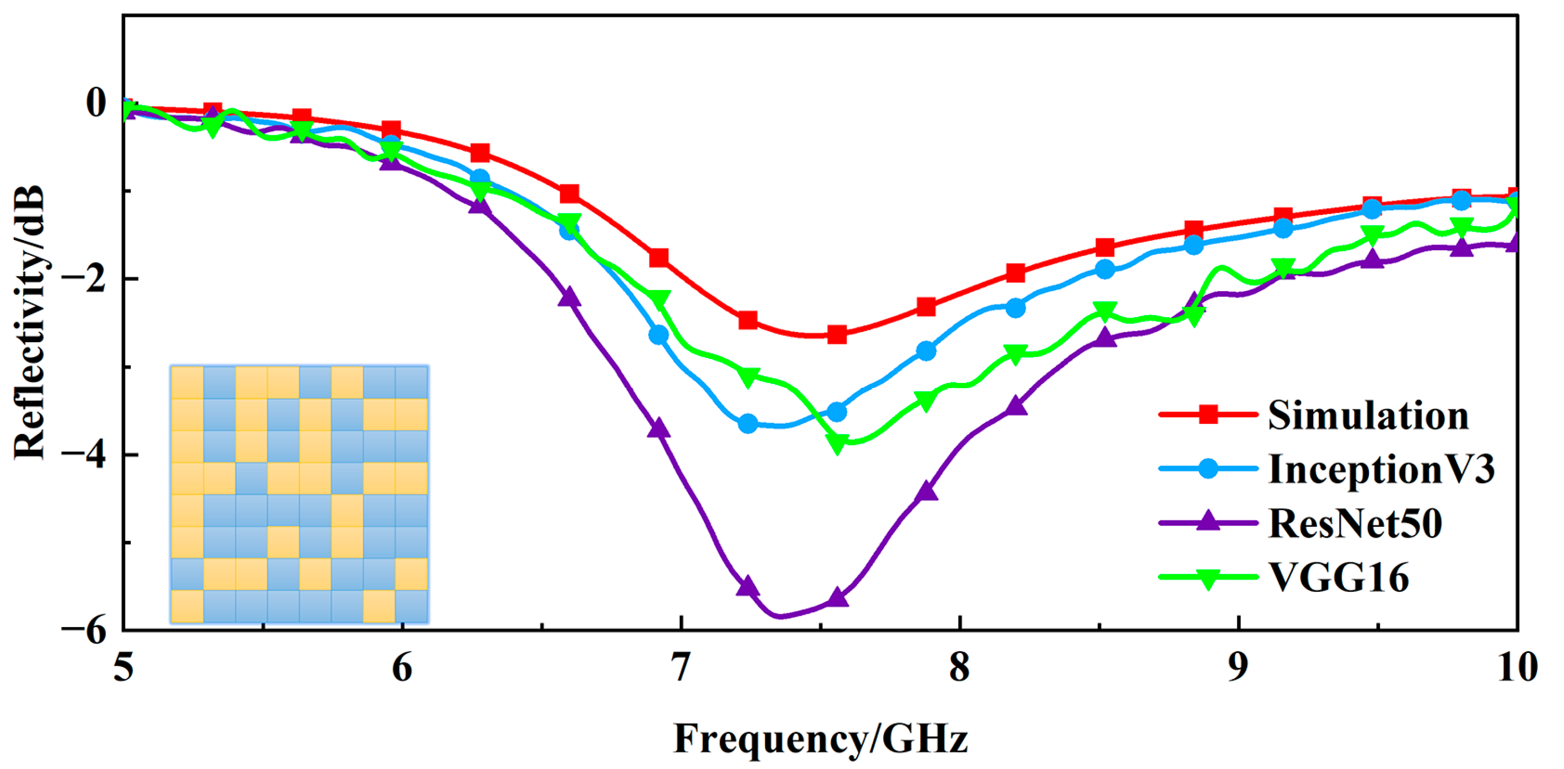
By minimizing the MSE loss function, the model aims to make the predicted values as close as possible to the actual values, resulting in accurate regression predictions. Under the same conditions, we use three pre-trained models, i.e., InceptionV3, ResNet50, and VGG16 to build the forward prediction network, respectively, and then train the network. The comparison of their loss value and average time is shown in

Table 1. Comparison of pre-trained models: InceptionV3, ResNet50, and VGG16.

Pre-Trained Model	Train Loss	Test Loss	Validation Loss	Average Time
InceptionV3	0.7051	1.3071	1.2871	1 h 40 min
ResNet50	0.2699	1.2239	1.1355	2 h 23 min
VGG16	1.2312	1.4225	1.5815	3 h 37 min

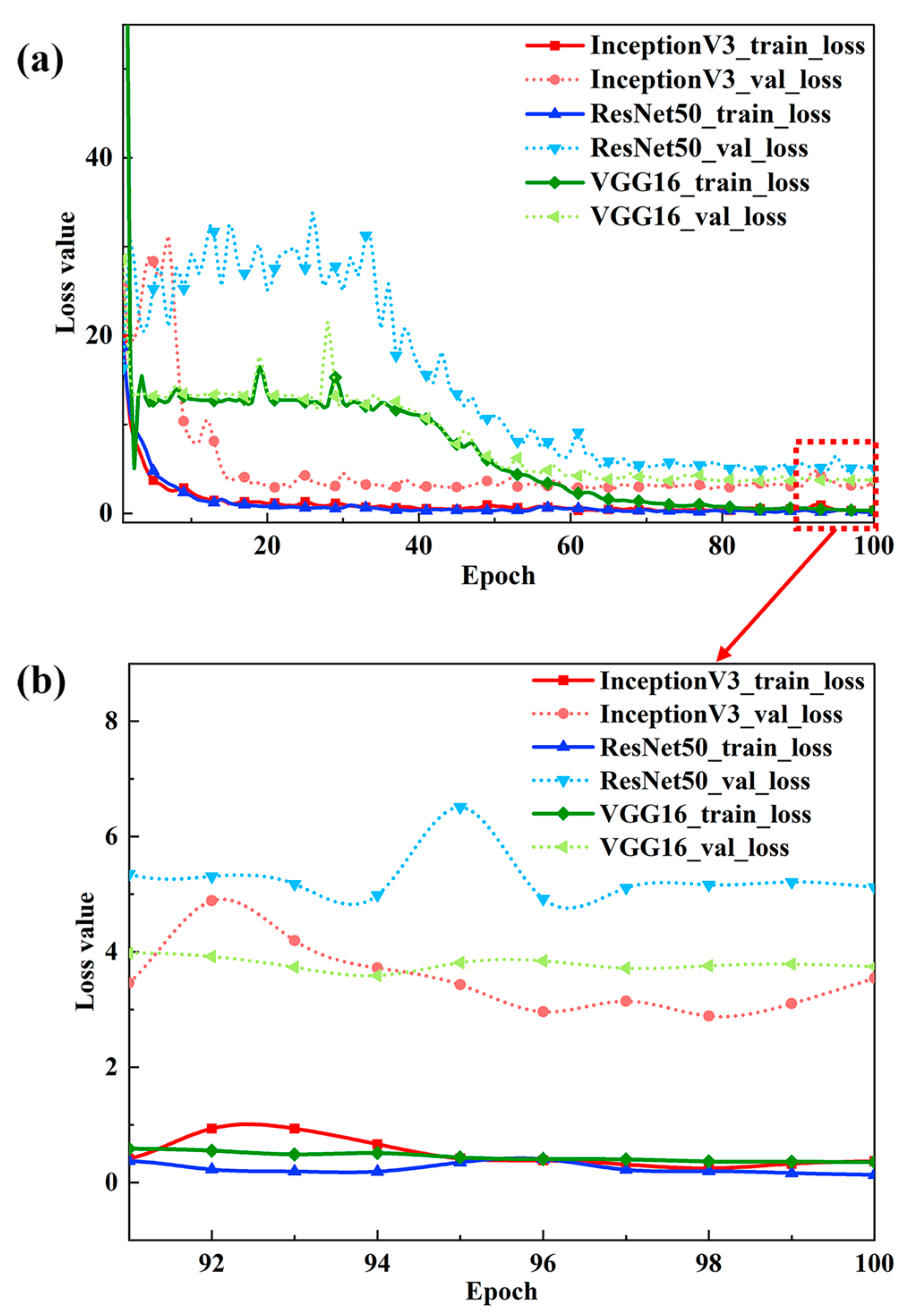
. Obviously, ResNet50 reaches the lowest loss, but meanwhile, it is the most time consuming. Figure 2 shows the loss function curves of the three models during the iteration process. On the one hand, InceptionV3 converges the fastest. On the other hand, InceptionV3 converges to a relatively low loss value, whether it is the loss function of the training or the loss function of the verification process.

In terms of model architecture, the Inception model uses multi-layer convolution and aggregation operations to extract features in the image, and uses a 1 × 1 convolution kernel to reduce the dimension to achieve parameter reduction. ResNet, on the other hand, solves the vanishing gradient problem and model degradation phenomenon by using residual connections, allowing the network to be deeper and producing operations similar to skip connections when adding new layers. In terms of the number of parameters, since the Inception network uses a 1 × 1 convolution kernel to increase or reduce the feature dimension, it has a small number of network parameters and is suitable for scenarios with limited computing resources. In contrast, ResNet’s residual connection module leads to a deeper network and requires more network parameters, thus requiring a larger dataset and longer training time to avoid overfitting. Due to the characteristics of fewer parameters and the high computational efficiency of the Inception network, it is suitable for deployment on resource-constrained devices, and performs well for complex image classification problems while maintaining performance. Overall, VGG16 is suitable for small-scale image classification tasks due to its simple architecture, which employs stacked convolutional and pooling layers for feature extraction and a fully connected layer for classification. With the concept of residual blocks having been introduced, which can train deeper neural networks and avoid the problem of vanishing gradients, ResNet50 is usually used to solve large-scale image classification problems. As for InceptionV3, its outstanding performance in dealing with complex image problems is essential in this paper. Considering the above factors, InceptionV3 is applied to complete the network architecture and subsequent program design.

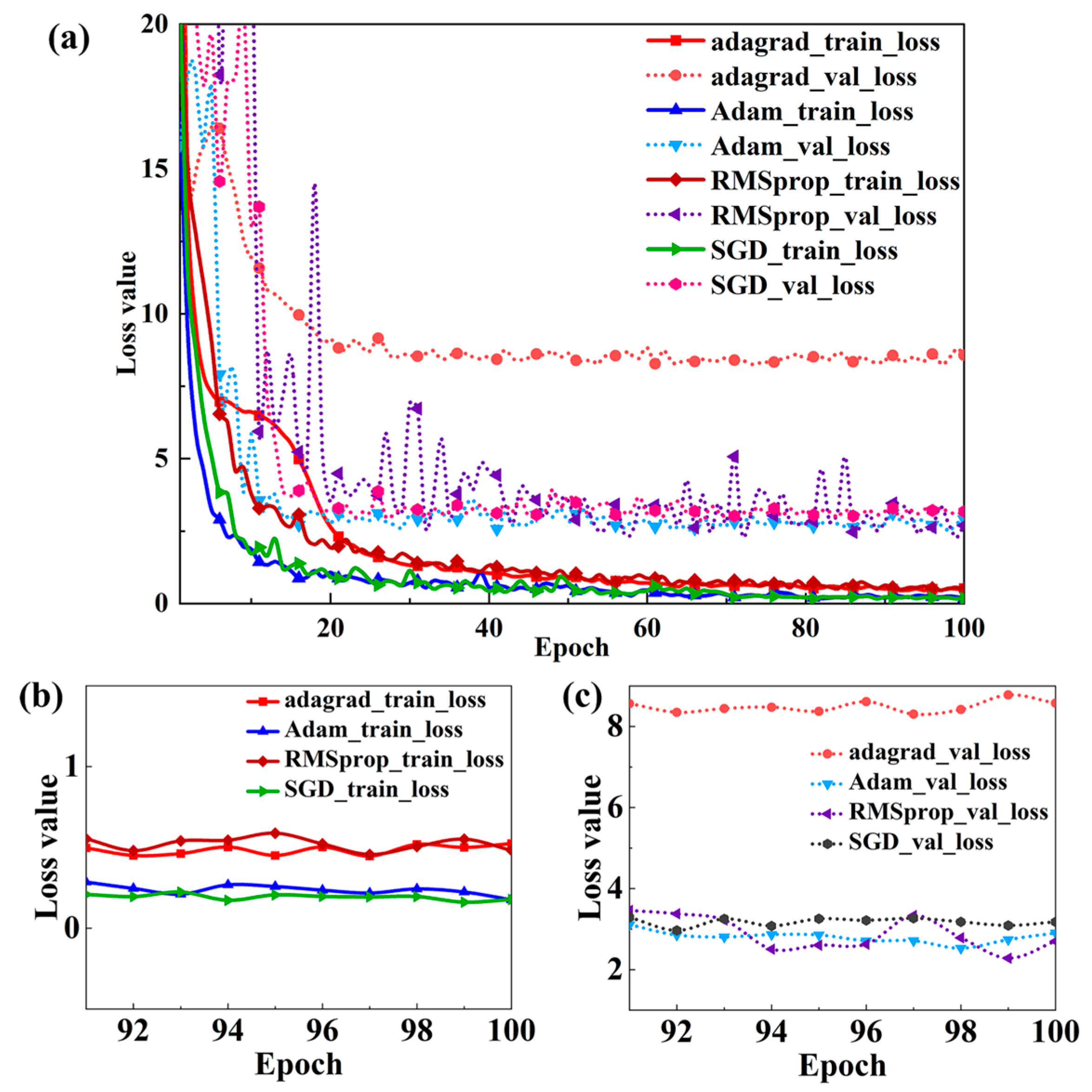
We tried a variety of optimizers (respectively, as follows: AdaGrad, Adam, RMSprop, and SGD) and compared them in Figure 3. The full 100-iteration process shows the fastest convergence of loss values for Adam and the SGD. For the training loss, there is little difference, but for the validation loss, Adam is better than the SGD. In addition, from the perspective of the theory, the SGD only uses the gradient information of a single sample to update the parameters, so it has a high noise value and a large floating range of variance, which makes it difficult to achieve the global optimal solution in the training process. The Adaptive Moment Estimation optimization algorithm (Adam) dynamically adjusts the learning rate of each parameter using first-order gradients and second-order moment estimates, and thus expedites the convergence speed. One of its advantages is that after correction, the learning rate has a certain range in each iteration, which makes the parameters relatively stable. The parameter update formula is as follows:

$$m_t={\beta }_1{m}_{t-1}+(1-{\beta }_1)g_t$$

(3)

$$v_t={\beta }_2{v}_{t-1}+(1-{\beta }_2)g_t^2$$

(4)

$${\stackrel{\wedge }{m}}_t={\displaystyle \frac{m_t}{1-{\beta }_1^t}}$$

(5)

$${\stackrel{\wedge }{v}}_t={\displaystyle \frac{v_t}{1-{\beta }_2^t}}$$

(6)

$${\theta }_{t+1}={\theta }_t-\frac{\alpha }{\sqrt{{\stackrel{\wedge }{v}}_t}+\epsilon }{\stackrel{\wedge }{m}}_t$$

(7)

In Expressions (3)–(7), $m_t$ and $v_t$ are the first and second moment estimates of the gradient, respectively, which can be seen as approximations to the expectation $E[g_t]$, $E[g_t^2]$, and ${\stackrel{\wedge }{m}}_t$ and ${\stackrel{\wedge }{v}}_t$ are corrections of $m_t$ and $v_t$, such that an unbiased estimate of the expectation can be approximated. As shown in Figure 3, the Adam optimizer outputs the lowest loss and converges, and its training loss is approximately a straight line equal to 0. We finally choose the Adam optimizer, which combines the advantages of AdaGrad and RMSProp optimizers [33].

2.3. CDCGAN

The goal of a generative model is to study a collection of training examples and learn the probability distribution that generated them. Generative Adversarial Networks (GANs) are then able to generate more examples from the estimated probability distribution. GANs have shown to effectively generate artificial data indiscernible from their real counterparts [34], especially to generate realistic high-resolution images. To improve the network structure of GANs, a deep convolutional generative adversarial network (DCGAN) is proposed [35]. The generator and discriminator of the DCGAN are both composed of convolutional neural networks. At the same time, the DCGAN improves the structure of the convolutional neural network, and is improved typically of the GANs model. Supervised learning with the CNN and unsupervised learning with the GAN are combined to form a network structure with stable training. It replaces any pooling layers with strided convolutions and fractional strided convolutions, uses Batch Normalization (BN) in both the generator and the discriminator, and removes fully connected hidden layers for deeper architectures, which alleviate the problem of model collapse and effectively avoid the oscillation and instability of the model [36].

In our research, we utilize a conditional deep convolutional generative adversarial network (CDCGAN) model, which employs conditional information to control the training of the GAN network. The conditional generative adversarial network (CGAN) is a conditional model obtained through introducing a conditional extension into the GAN, and the CDCGAN is a combination of the DCGAN and CGAN. This enables the network to generate images that align with the given conditional information. To incorporate the conditional data into the input, we opt to reshape both the conditional data and feature data into a 64 × 64-sized num.py array. Following this, the data are normalized to have a mean value of 0 and a variance of 1. The normalized data are then combined through matrix multiplication to create the input. Similarly, to ensure that the conditional data have a consistent impact on the input of the generation network, the input data undergo the same pre-processing steps. The hyperparameter settings for generating and discriminating networks are shown in

Table 2. Hyperparameters of CDCGAN.

Hyperparameter	Generator	Discrimator
Learning rate	10−4	10−4
Batch size	128	128
Optimizer	Adam	Adam
Activation function	Leaky ReLU and tanh	Leaky ReLU

.

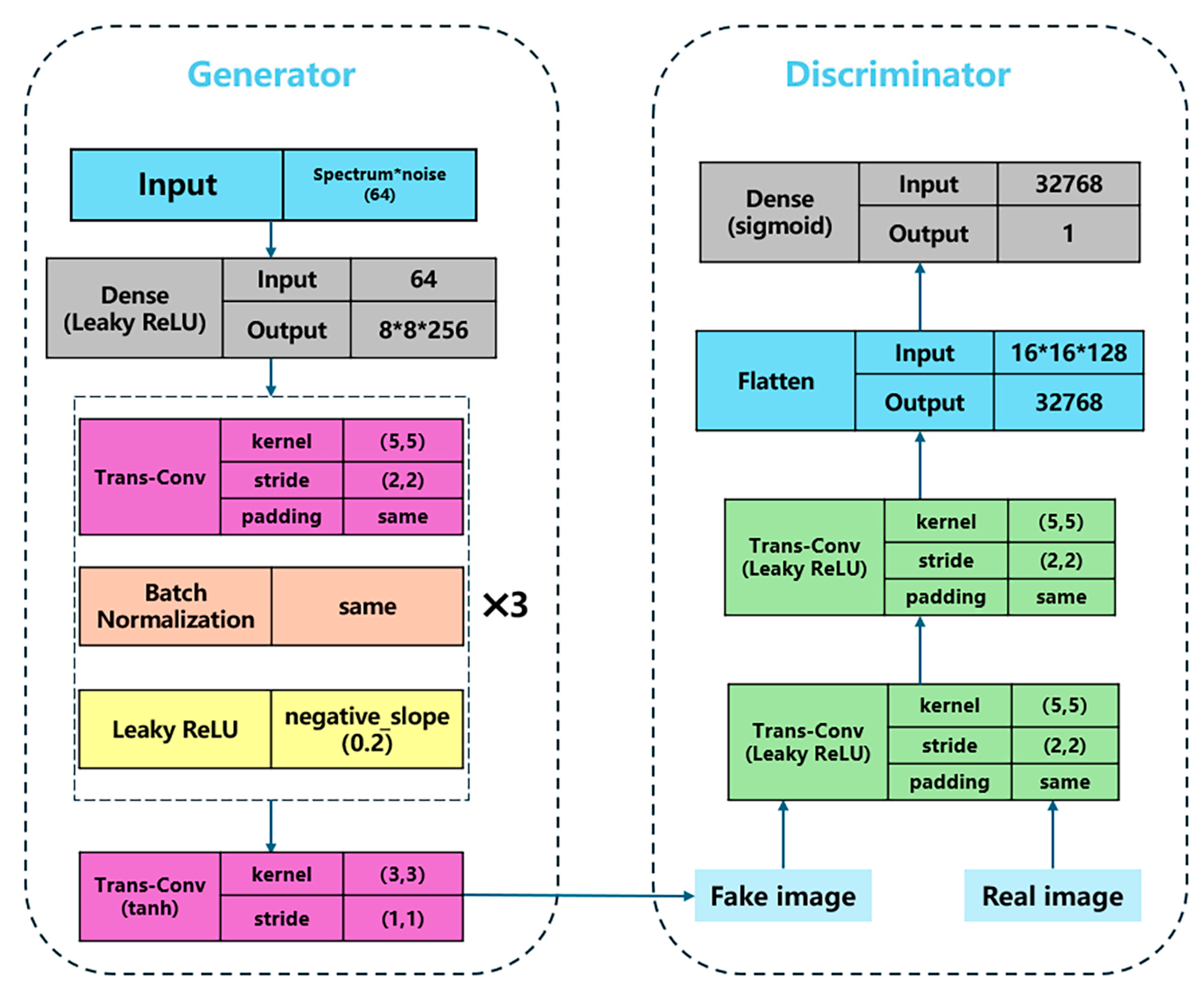
Figure 4 presents the Generator and Discriminator architecture of the CDCGAN. In the CDCGAN, the generator network takes reflection curves and Gaussian noise as inputs. A dense layer first transforms this combined latent vector into a three-dimensional feature tensor. This tensor is then processed through three successive transposed convolutional layers, progressively up sampling it to generate image data approaching the target dimensions. Batch normalization layers and Leaky ReLU activation functions are employed after these transposed convolutions to maintain stability during training. The final transposed convolutional layer in the generator uses a tanh activation function, mapping the pixel values of the generated output (the Fake Image) to the range [−1, 1], ensuring consistency with the pixel range of the real image data. The discriminator network receives both the generated fake images and real images as input. It processes them through two convolutional layers followed by a flatten layer, extracting features and converting the multi-dimensional feature maps into a one-dimensional vector. Finally, an output layer utilizing a sigmoid activation function maps this vector to a probability score between [0, 1], representing the likelihood that the input data are a real image.

CDCGAN ultimately needs to optimize the following objective function [37]:

$$\underset{G}{\min }\underset{D}{\max }V(D,G)=E_{x~P_{data}(x)}\left[\log D(x | y)\right]+E_{Z~P_Z(Z)}\left[\log (1-D(G(z | y)))\right]$$

(8)

In Expression (8), $E_{x~P_{data}(x)}\left[\log D(x | y)\right]$ indicates the probability that the data x are determined as the real data after the data x and the condition y are put into the discriminator D. $E_{Z~P_Z(Z)}\left[\log (1-D(G(z | y)))\right]$ denotes the probability that the samples, which are generated after the random noise z and the condition y are put into the generator G, are determined as the real data [31]. The goal of D training is to maximize $\log D(x | y)$ and $\log (1-D(G(z | y)))$, while the goal of network G training is to minimize $\log (1-D(G(z | y)))$. Expression (8) is the maximum optimization and minimum optimization, which cannot be completed within one step. In essence, the training method of G and D is a separately and alternatively iterative process, in which we keep D or G unchanged and then update the parameters of another network. The result of the training was that G can simulate the distribution of real samples and generate more authentic and reliable data.

3. Results

3.1. Forward Prediction Network

The training result about the TLN model is shown in Figure 5, and the pattern in the lower left corner is an example of the input meta-atom. Although we only use 2048 sets of data for training, the results still show a high accuracy. We use the trained model to predict a randomly selected sample and compare the predicted result with the reflection spectrum curve of the corresponding structure simulated in HFSS. The models trained using three pre-trained models, InceptionV3, ResNet50, and VGG16, are relatively accurate in predicting the trend of reflectivity curves. In general, the prediction result of InceptionV3 is in better agreement with the simulation curve than the other two models, especially given that its prediction accuracy of amplitude is relatively higher.

3.2. Inverse Design

Based on the CDCGAN method, a broadband metasurface absorber was reverse designed, as shown in Figure 6. For the application target of the C-band, we hope to obtain the reflectivity performance as shown by the input curve in Figure 6c. After CDCGAN training, the meta-atom as shown in Figure 6a was obtained through reverse design, and the black clumps represent the resistance film, with a square resistance of 400 Ohm/m². The output curve of Absorber I has good agreement with the original input one in Figure 6c, which can achieve an absorption effect of less than −8 dB in the range of 6.5–8 GHz, and the absorption performance reaches less than −15 dB near the resonant frequency point of 7 GHz. Figure 6b shows the 3D view of Absorber I using 2 mm thick F4B as the substrate. Considering the application requirements of the X-band, Absorber I is optimized to Absorber II through a lightweight design process. Specifically, the F4B substrate was replaced by thinner FR4 with a thickness of 0.15 mm, and a 1.5 mm thick Nomex honeycomb with a mass density of only 48 kg/m³ was used as the dielectric layer. The honeycomb has a dielectric constant of 1.07, close to the value of air. Figure 6d shows the simulated reflectivity results of Absorber II, from which can be seen that the lightweight treatment can achieve an absorption bandwidth below −8 dB at 9–12 GHz.

3.3. Experimental Verification

To further verify the model, we also fabricated a corresponding metasurface prototype, as shown in Figure 6b, whose patterns and structural parameters were consistent with the model of Absorber II in Figure 6b. The metasurface absorber consists of 17 × 17 meta-atoms with a side length of 170 mm. Figure 7a is a photograph of the measurement setup. The reflectivity of the absorber is measured using a free-space measurement in the anechoic chamber. Two-step calibration is required before measurement. Initially, the noise floor is measured by recording the reflection from the anechoic chamber in the absence of any sample. Then, an aluminum plate with the same size as the absorber sample is placed in the anechoic chamber and the reflection (R_m) is measured. After the calibration is completed, the reflection (R_a) is measured by replacing the aluminum plate with the fabricated absorber. The difference (R_a − R_m) of both the reflection coefficients gives rise to the actual reflectivity from the fabricated absorber. We measured the reflectivity of the sample and compared it with the simulation result, as shown in Figure 7c. The fabricated metasurface absorber exhibits wideband absorption performance, which can achieve below −8 dB over the microwave frequencies ranging from 9.5 to 11.8 GHz. The curve of the experimental measurement results is rather fluctuating, and the overall reflectivity is lower than that of the simulation results. Comparing results from the experiment and simulation, slight differences in the amplitude of the absorption peak exist, which result from the electromagnetic parameter error of the sample and the influence of the experimental environment. However, the effective absorption frequency bands are also corresponding in a wide band and the trends in reflectivity are quite similar.

Finally, a comparison between our study and previous works is given in

Table 3. Performance comparison of this work and other different types of metasurface designs.

Reference	Network	Number of Samples	Epochs	Training Parameter	Function
[26]	Transfer learning	50,000–70,000	10,000	0–360° phase and 10 GHz	2D focusing and abnormal reflection
[38]	IMNNM	10,180	300	3.5–5.5 GHz	Polarization control
[39]	DNN	2000	5000	Resonance frequency (6.5/11.5/24 GHz, etc.)	Absorption
[40]	RGAN	15,000	10,000	6–17 GHz	Absorption
This work	Transfer learning + CDCGAN	2000	100	5–10 GHz	Absorption

. Based on the comparison, this work, by combining transfer learning (TL) and CDCGAN architectures, can achieve a rapid reverse design of a broadband metasurface absorber based on a small amount of data, which is crucial for applications such as the rapid optimization of electromagnetic absorption structures.

4. Discussion

While the proposed inverse design framework demonstrates significant advantages in automating and accelerating the metasurface absorber design process, several practical aspects warrant further discussion. First, it is acknowledged that conventional design methods, such as those based on equivalent circuit models or parametric optimization of regular geometries, can achieve moderate bandwidth absorption with relatively low computational complexity. However, these approaches often require substantial human expertise and are less scalable for complex design objectives such as multi-band operation or dynamic reconfigurability. Although more computationally involved in its initial stages, the methodology presented in this work significantly shortens the design cycle and provides a powerful tool for generating non-intuitive, high-performance architectures that are difficult to realize using conventional techniques.

With regard to fabricability, the pixelated metasurface structures proposed in this study are particularly well suited for microwave frequencies, where the required feature sizes are compatible with cost-effective fabrication techniques such as printed circuit board etching or laser ablation. However, extending this approach to higher frequencies, such as terahertz or infrared regimes, would require nanoscale patterning precision. This level of precision currently depends on advanced lithographic techniques, which may introduce practical limitations related to cost and scalability. Therefore, the proposed methodology is especially advantageous for microwave applications, where design flexibility and rapid prototyping are crucial.

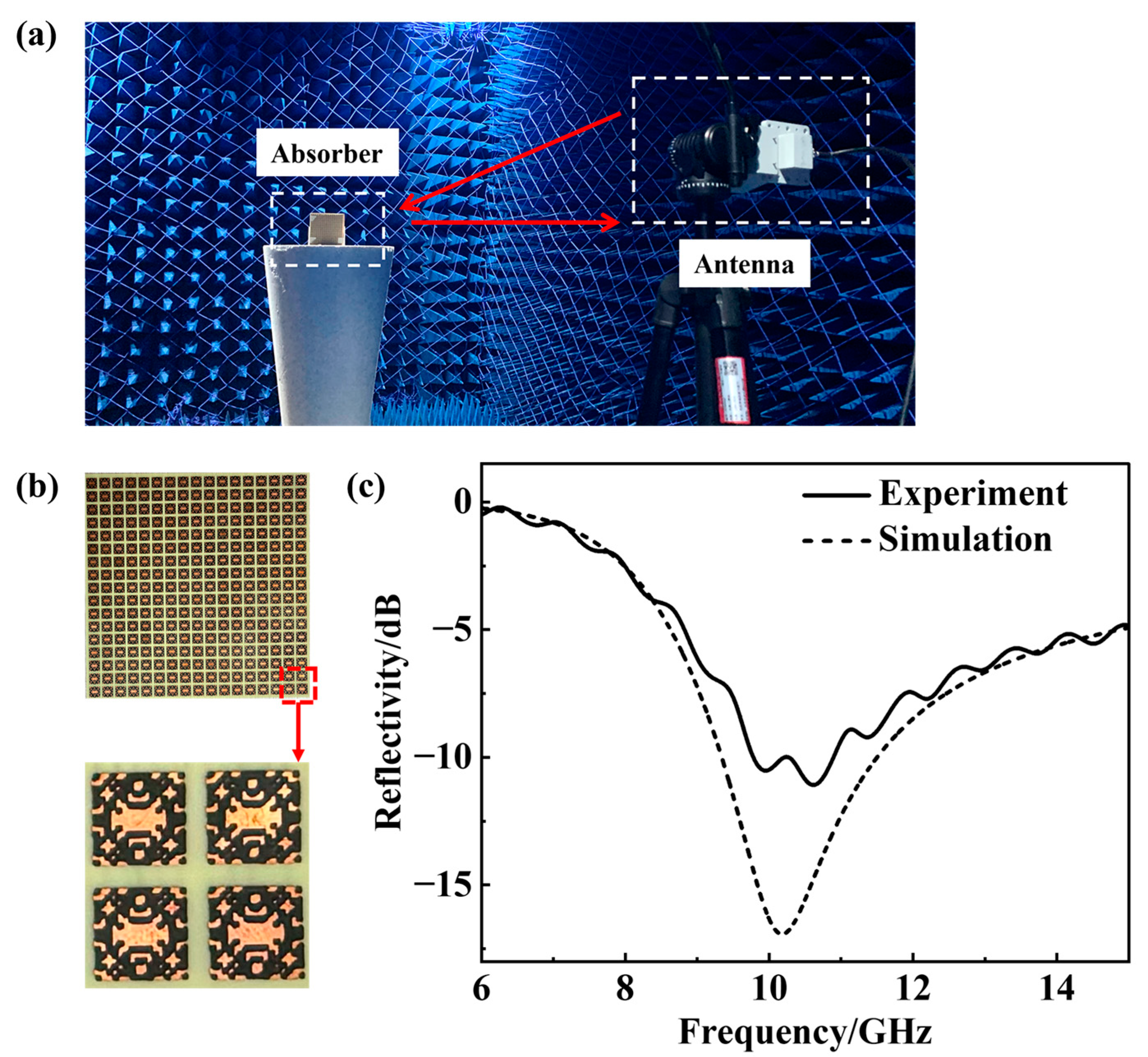
Overall, it should be emphasized that the primary contribution of this work lies in introducing a new inverse design paradigm based on transfer learning and conditional generative adversarial networks, rather than in presenting a specific absorber device for immediate practical application. The fabricated prototype serves as a proof-of-concept validation within the microwave range, demonstrating the feasibility of the algorithm-generated designs. This approach opens a route for a computationally efficient and generative design of functional metasurfaces, with potential for extension to broader frequency ranges and more complex specification constraints.

5. Conclusions

In this paper, we propose a fast inverse design method based on a transfer learning network and CDCGAN, which is experimentally verified for metasurface absorber design with a lower simulation cost and relatively high design accuracy. The forward neural network transfers the knowledge of image recognition to the reflectivity curve prediction of the metasurface. The InceptionV3 pre-trained model is chosen to build the TLN after considering the computational power and model accuracy limitations. Additionally, the network is fine-tuned using optimization algorithms, with the Adam optimizer being selected after comparison. A conditional deep convolution GAN is built, allowing the generation of desirable meta-atom patterns by inputting a reflectivity curve. Using the database established by the TLN model, given an expected reflectivity curve, the CDCGAN can generate an eligible 1/4 pattern, with which we use to design a full image of the metasurface. In addition to this, we also have fabricated the corresponding metasurface absorber, and measured its reflection curve. The measured result matches the simulated reflectivity well in the operated frequency band. While this approach provides an efficient framework for static wideband absorbers, its architecture inherently supports future evolution toward intelligent reconfigurable systems. By incorporating tunable elements like varactor diodes or MEMS devices into the pixelated resistive films, our method could be extended to achieve dual-band frequency agility, allowing dynamic absorption tuning between distinct operational bands without structural modifications. Such advancement would align our computational framework with next-generation needs for adaptive metamaterial systems.