Evaluating the educational impact of the developed interactive software models is a key point in determining their applicability and usefulness in the learning process. In the context of error correction codes, characterized by high theoretical abstraction and algorithmic complexity, such as cyclic codes, it is important to check whether the use of interactive tools facilitates the understanding of basic concepts and supports the mastery of specific coding principles. The evaluation aims to examine the extent to which the developed models facilitate the learning process and increase student engagement. In addition, it includes a review of the usability of the interface, compliance with the previously set learning objectives, and subjective impressions of users regarding the effectiveness of the model. Such an evaluation could serve as a basis for identifying opportunities for improvement and for adapting the models to different learning contexts.
3.2.1. Statistical Analysis of the Educational Effectiveness
Cyclic codes are studied within the course “Reliability and Security of Computer Systems”, taught in the third year of the Computer Systems and Technologies major at the University of Ruse “Angel Kanchev”. The developed interactive software model for studying cyclic codes using the polynomial method was implemented in the educational process in 2021 and is actively used at the time of writing this article as an alternative to the traditional written approach to solving problems. The second software model, based on a linear feedback shift register, was also introduced in 2021, but it serves primarily a demonstrative function, as it presents a new approach that has not been applied in the form of written exercises.
Conducting a pre-test as a way of establishing the initial academic level in the present study was not possible due to the specifics of the study, namely the formation of groups from different academic periods. This approach was necessary to comply with the principle of equality between students within the same cohort during the learning process. It is important to note that the idea of forming a control and experimental group arose only at the stage of implementing the interactive models. This means that during the training of the students from the control group, their participation in an experimental study was not foreseen, and their results were included post hoc. To avoid creating inequality within the same cohort, the experimental group was formed in a subsequent academic period, while the control group covered an earlier cohort. Although the groups are from different academic years, they are part of the same educational program, have gone through the same curriculum with the same teachers, and are educated under comparable institutional conditions.
Conducting a pretest as a way to establish the initial academic level in this particular case is not possible due to the specific conditions of the study, namely the formation of groups from different academic periods. This approach is required in order to comply with the principle of equality between students from the same stream during the educational process.
Within the framework of this study, the initial academic level of the participants was assessed by using the average grade point from the previous two semesters as an alternative to a pretest. Although this indicator does not directly measure knowledge on a specific topic, it provides a reasonable idea of the general academic level of the students. This allows for assessing the preliminary comparability between the groups and controlling for the possible effect of initial differences in preparation when interpreting the results after training. The choice to use grades from the last two semesters as an indicator of the initial academic level assumes that this period reflects the current state of student success and ensures sufficient completeness and comparison of data for all participants in the study. The data on the average grade were extracted from the examination protocols provided by the faculty office of the university.
To measure the final state of the participants in the study, the results of control papers (tests) on the topic of cyclic codes by the polynomial method, conducted by the training format of each of the groups, were used. Students from the control group conducted control papers in traditional written form, while participants from the experimental group used the interactive software tool, in the “Test” mode. In this mode of working with a model, restrictions have been introduced aimed at simulating conditions comparable to those of the written form—including a limited number of attempts to start a task and the impossibility of re-executing the model in case of an error. In this way, it is assumed that comparability, control, and objectivity are ensured in the assessment of the two groups, regardless of the differences in the teaching method used. The collection of data from the control works was carried out with the assistance of the teachers who taught the course. The tasks on cyclic codes with a linear feedback shift register are not included in this study, because they have no analogue in the control group, i.e., they were not studied in written form.
Before conducting comparative tests for the initial and final state, it is necessary to present information about the samples from both groups through descriptive statistics and frequency distribution. This allows for assessing the distribution of the results, detecting possible deviations or extreme values, and ensuring that the groups are comparable. For the statistical processing, the specialized software product SPSS v26 was used, which has found wide application in scientific fields when performing various types of statistical analyzes [
38].
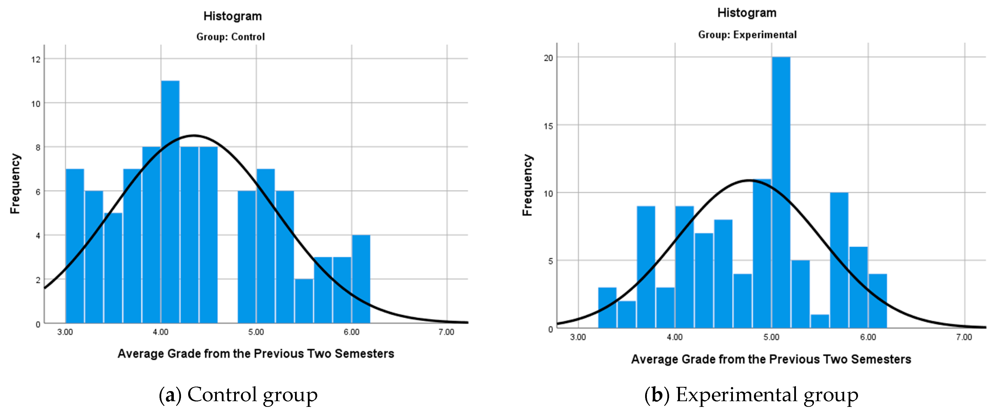
The number of participants in the control group is 91 students (from 2019 to 2020), and in the experimental group—102 students (from 2021 to 2025). The results of the descriptive statistics for the two groups at baseline are given in
Table 4, and
Figure 23 also shows the frequency distribution of the grades from the previous two semesters by group.
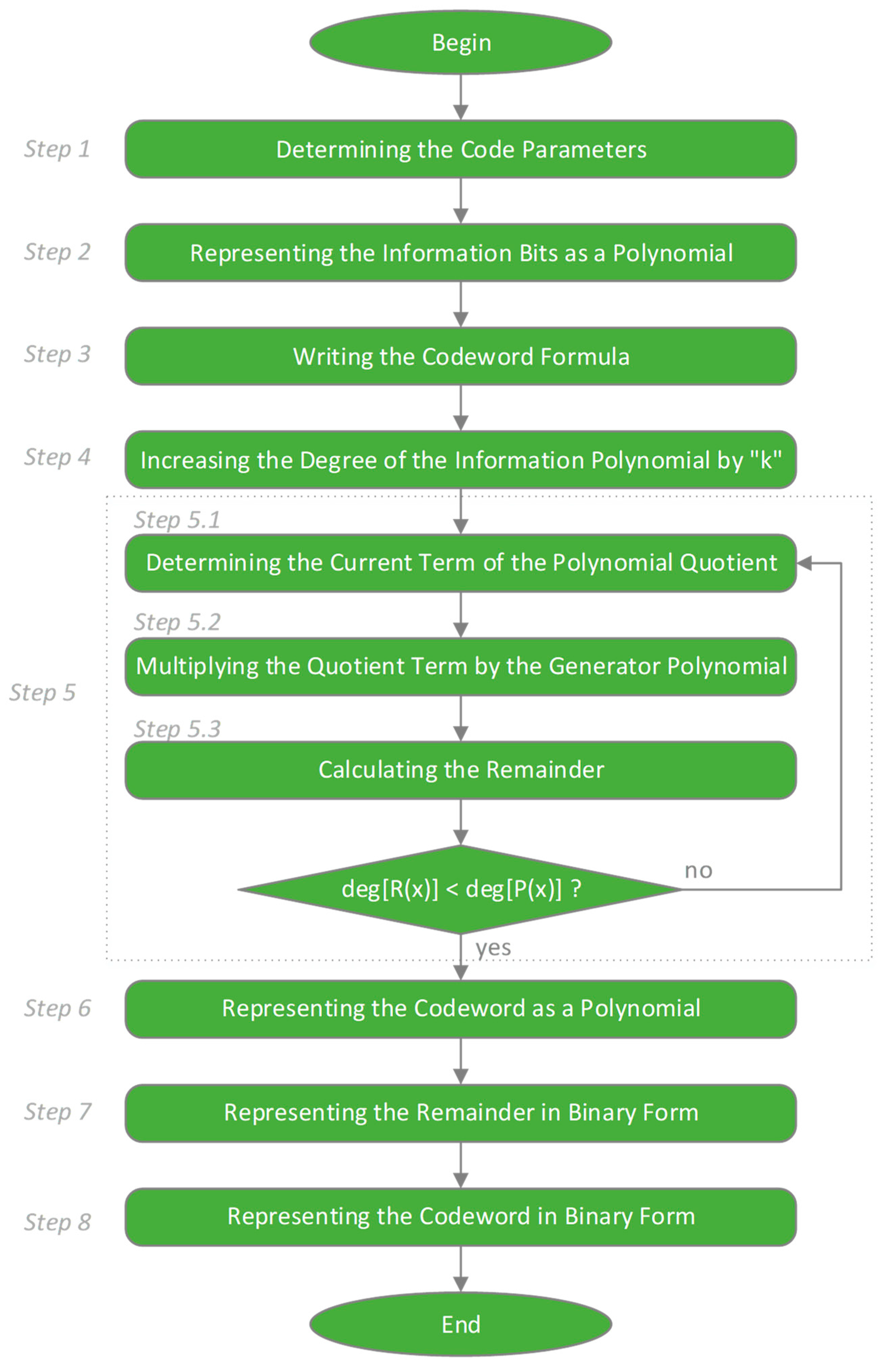
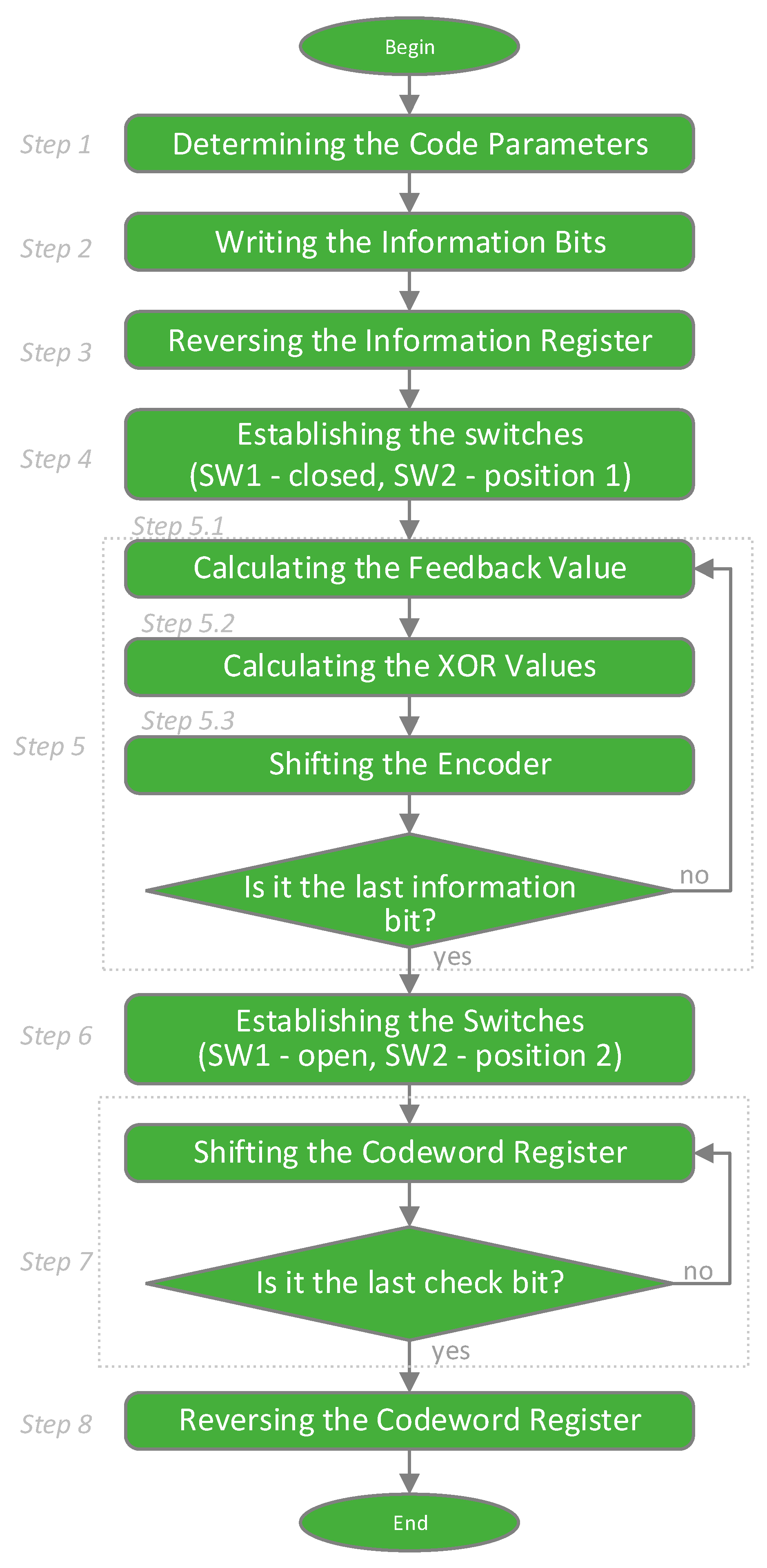
At this stage of the study, a statistical test is performed to determine whether there is a significant difference in the average grade of the two groups at the beginning of the experiment, in order to determine whether the students were at a similar academic level before the application of the software models. The comparison of the overall academic level between the control and experimental groups was done through hypothesis testing, following the general algorithm shown in
Figure 24.
- -
Formulation of the hypotheses and .
- ○
Null hypothesis —There is no statistically significant difference;
- ○
Alternative hypothesis —There is a statistically significant difference.
- -
Determination of the risk of error α
The risk of error or significance level (α) represents the probability of rejecting the null hypothesis when it is actually true. This value is determined in advance by the researcher and is used as a criterion for statistical significance. In practice, the most commonly used values for α are 0.05 or 0.01, which corresponds to a 5% or 1% acceptable risk when deciding to reject the null hypothesis [
39]. In this study, a significance level of α = 0.05 was adopted.
- -
Test Selection
The choice of an appropriate test for comparison depends on whether the data in the two groups are normally distributed. In this regard, a check for normality of the data distribution was performed using the Kolmogorov–Smirnov test, which is one of the widely used methods for assessing the correspondence between the empirical distribution of sample data and the theoretical normal distribution. The test compares the cumulative empirical function with the expected cumulative function under the normal hypothesis and allows one to assess whether the deviations are statistically significant [
40]. The results of the normal distribution test are given for the control group in
Table 5 and for the experimental group in
Table 6, respectively.
According to the results obtained from
Table 5 for the control group, it can be seen that the
p-value (Asymp. Sig. 2-tailed) = 0.0798 is greater than the significance level α = 0.05. This means that there is not enough statistical evidence to reject the hypothesis of normal distribution, i.e., it is assumed that the data are normally distributed. The situation is similar for the experimental group (
Table 6), where the
p-value (Asymp. Sig. 2-tailed) = 0.089 is greater than the significance level α = 0.05. After it has been established that the data in both groups follow a normal distribution, according to the algorithm in
Figure 24, a parametric test should be conducted for a statistical comparison of the mean values between the control and experimental groups.
An independent samples
t-test for two samples (also known as Student’s
t-test) was chosen, which is a classic method for assessing whether the difference between two means is statistically significant. The results of the
t-test are given in
Table 7.
According to the results of
Table 7, it was found that the
p-value (Sig. 2-tailed) = 0.000 is less than the significance level
; therefore, the hypothesis
is accepted, which states that there is a statistically significant difference in the average grades of the control and experimental groups. This suggests that the students from the control group had better academic achievements before the start of the experimental study. In such a situation, it is methodologically incorrect to make a direct comparison of the final results, since the reported differences could be due not only to the training method used, but also to the prior academic preparation of the participants.
The presence of a statistically significant difference in the initial academic level between the groups necessitates the use of a statistical control method, such as ANCOVA, in order to guarantee objectivity in the interpretation of the training results and to assess the real impact of the software tool used on academic success. The ANCOVA method allows for adjusting the final results so that the comparison between groups considers the initial differences and reflects the effect of the applied training approach.
ANCOVA (analysis of covariance) is a statistical method that allows for assessing the effect of an independent variable on a dependent variable, while simultaneously controlling for the influence of external factors (covariates) [
41]. In the context of the present study, the method is suitable for assessing the impact of the software tool on the academic performance of students (results of control work on cyclic codes), taking into account their previous average grade. This provides a correction for the initial differences between the groups and allows for a more objective assessment of the effectiveness of the used training approach compared to the traditional method.
Within the framework of the analysis, the following variables are included in the ANCOVA model:
- -
Dependent variable—the assessment from the control work on cyclic codes;
- -
Independent variable—the group, i.e., the training method used (traditional or software);
- -
Covariate variable—Average grade from the previous two semesters.
Before applying ANCOVA, it is necessary to check the homogeneity of variances between groups—one of the main assumptions for the validity of the analysis [
41]. Violating it can lead to inaccurate results. For this purpose, the Levene test is used, which assesses whether the variations of the dependent variable are approximately equal in the compared groups. The results of the Levene test are given in
Table 8.
The results of the Levene test (
Table 8) for homogeneity of groups show that the
p-value (Sig.) = 0.233 is greater than the selected significance level α = 0.05. It follows that the assumption of homogeneity of variances is met, and the ANCOVA test can be continued.
The following general interpretation of the results of the ANCOVA test (
Table 9) can be made:
- -
Corrected Model. This parameter represents the overall characteristics of the ANCOVA model. The obtained results F = 45.143, p (Sig) = 0.000 < 0.001 < α = 0.05 show that the model is statistically significant. This means that the included predictors (AverageGrade and Group) explain a significant part of the variation in the test results (Cyclic Code Test Scores).
- -
AverageGrade. It expresses the influence of the covariance effect or in the current case the influence of the initial academic level (grade point average of the previous two semesters). With a result of F = 67.884 and p (Sig) = 0.000 < 0.001 < α = 0.05, which means that the grade point average has a highly significant influence on the results.
- -
Group. The effect of the factor “Group” (reflecting the teaching methodology) is also statistically significant: F(1.190) = 6.061, p = 0.015 < α = 0.05. This means that the teaching method has an impact on the test results, even when controlling for the influence of the average grade from the previous two semesters.
In order to determine the effect of the factor “Group” more precisely, it is necessary to analyze the adjusted means of the dependent variable (cyclic code test scores) for each group, after controlling for the effect of the covariate (average grade). SPSS provides the ability to automatically output these values.
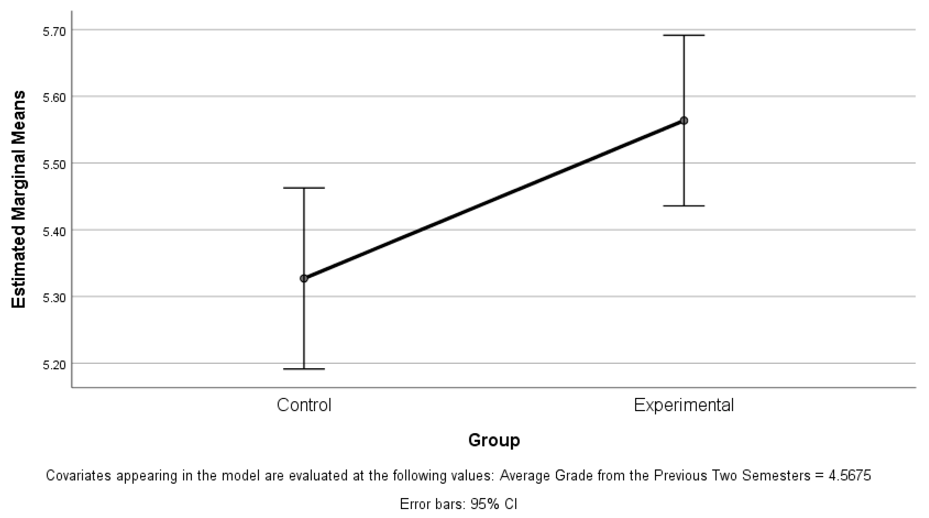
Table 10 and
Figure 25, respectively, present in tabular and graphical form the expected average values of the results of the control work on cyclic codes for the two groups, after accounting for the influence of the average grade from the previous two semesters.
According to the results in
Table 10, the value of the covariance (the average grade of the previous two semesters) is fixed at 4.5675 so that the two groups are compared at the same level of academic success. Under these conditions, the adjusted average value of the test scores for the experimental group is 5.564, which is 0.237 more than the control group. Although the difference seems small, it is statistically significant (
p = 0.015), as confirmed by the results in
Table 9, which indicates that it is not random.
The results of the analysis show that the use of software models in teaching, although leading to a relatively small increase in scores, has a positive effect on the assimilation of the learning material. The difference between the groups is not large, but it is statistically significant, which suggests that the introduction of such approaches can contribute to better student performance, especially in the long term.
3.2.2. Student Activity and Performance Analysis
In addition to the comparative analysis of academic achievements between the experimental and control groups, it is necessary to conduct a more in-depth study of the activity and effectiveness of students in the real use of the developed software models. Such an analysis allows tracking user activity, such as the number of solved tasks, average time for solving, and the degree of success, which provides an objective idea of the way in which students interact with the tool. The information obtained is of key importance for assessing the practical applicability of the software, its accessibility and pedagogical effectiveness in a real learning environment, as well as for identifying opportunities for its future improvement.
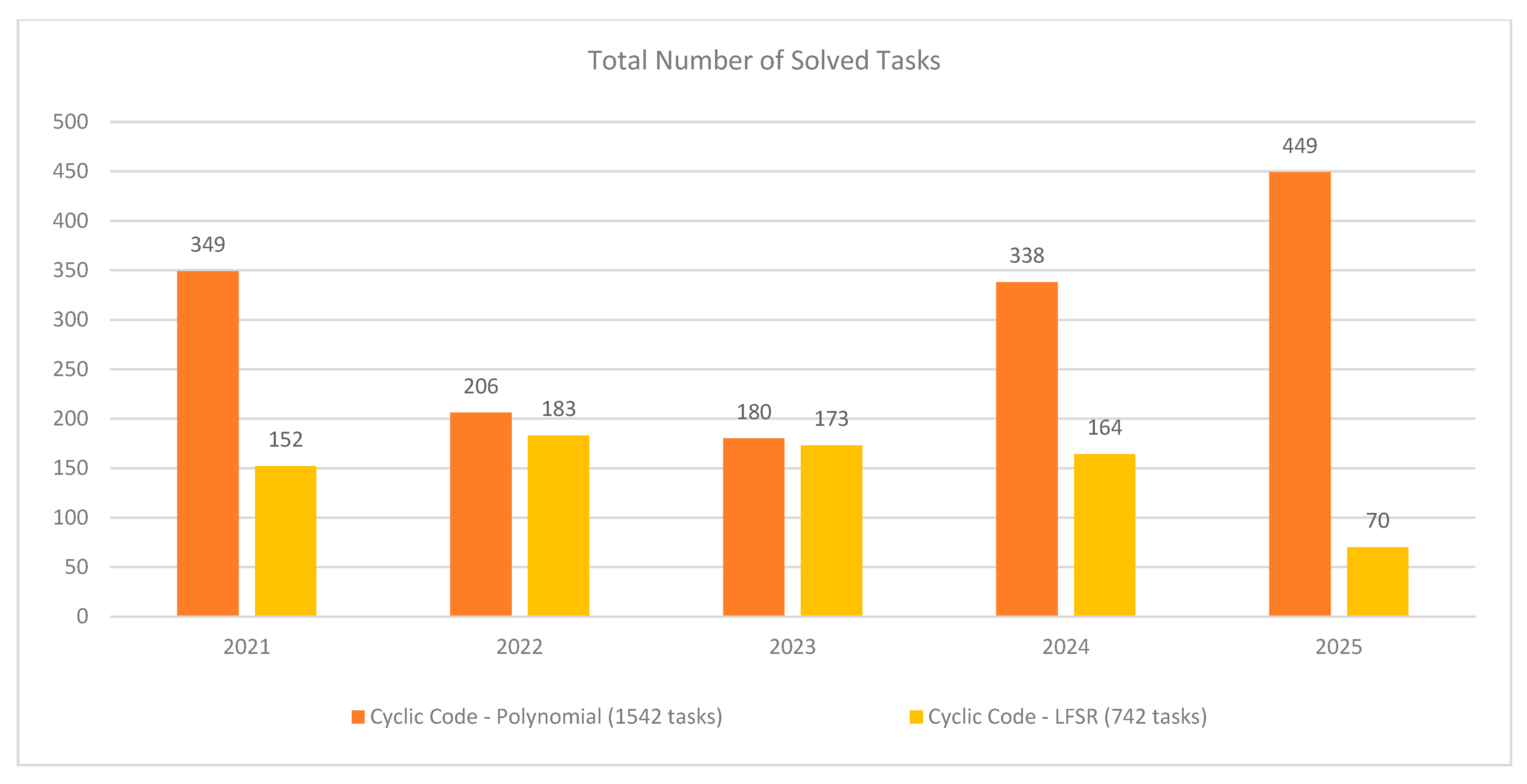
Figure 26 presents the total number of solved tasks by year with the two interactive models for solving cyclic code problems: cyclic code—polynomial and cyclic code—LFSR, for the period 2021–2025.
The Cyclic Code—Polynomial model demonstrates consistently higher activity in all years, reaching a maximum of 449 solved tasks in 2025 and a total of 1542 problems for the entire period. On the other hand, the Cyclic Code—LFSR model shows peak activity in 2022 with 183 solved problems, with the total number for the five-year period being 742 problems.
It is important to note that the LFSR-based model is not mandatory for use in the educational process. It is introduced mainly for demonstration—to present an alternative, machine-based approach to solving problems with cyclic codes. For this reason, its use is entirely at the students’ discretion, which also explains the significantly lower number of solved problems compared to the main Polynomial model, which is mandatory within the exam format.
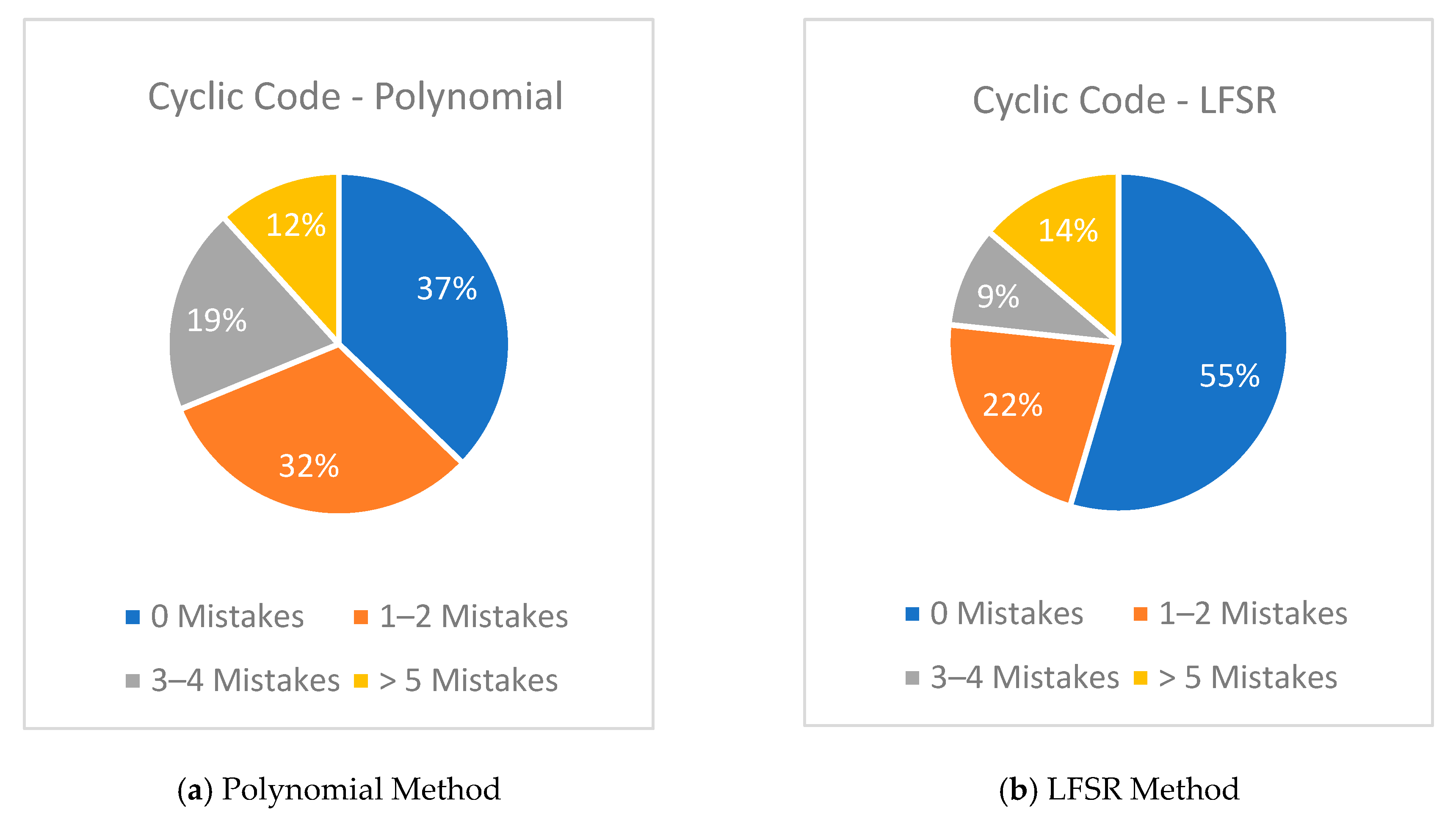
Figure 27 presents a comparative analysis between the Cyclic Code—Polynomial and Cyclic Code—LFSR models in terms of accuracy in solving problems, distributed according to the number of errors made: 0 errors, 1–2 errors, 3–4 errors, and more than 5 errors.
In the cyclic code—polynomial model, 37% of the problems were solved without errors, and 32% Unfortunately, we could not find the requested information either. The link to the publication does not contain this information.
https://mostwiedzy.pl/pl/publication/download/1/user-interface-prototyping-techniques-methods-and-tools_66913.pdfwith, accessed on 28 August 2025. 1–2 errors, which indicates a high level of learning and stable results for the majority of solutions. Only 12% of the solutions contained more than 5 errors, which indicates a relatively good effectiveness of the model as a training tool.
In the cyclic code—LFSR model, the share of problems solved without errors was even higher—55%—which indicates a significantly higher initial success rate. This result can be explained mainly by the fact that the complexity of the algorithm for solving problems using the LFSR model is significantly lower compared to the polynomial model. The simplicity of the method makes it easier for users to apply it, which leads to a lower number of errors when solving. However, the share of tasks with more than 5 errors is 14%, which is slightly higher compared to the polynomial model and is probably due to the rapid and careless execution of repetitive cyclic actions by students, typical of the more mechanical nature of the algorithm.
Figure 28 shows the distribution of the total time spent by each student working with the two interactive models. The data cover the individual total time for solving all tasks by a given student and are extracted through the functionality for automatic registration of tasks in the system. The polynomial model (Cyclic Code—Polynomial) has a higher median of engagement (about 60 min) and a more even distribution, which is in line with its main role in the learning process. On the other hand, the LFSR model has a lower median (about 20 min) and more limited use by some students, as it was designed for informative purposes and is used on a voluntary basis. The presence of outliers in both models indicates variations in the individual pace of work and the depth of engagement. The presented diagrams are not intended for direct comparison, but to illustrate the different patterns of interaction with each of the tools.
3.2.3. Student Satisfaction Analysis
Student satisfaction analysis is an essential component in assessing the effectiveness and acceptability of interactive software models used for educational purposes. The survey collects valuable information about students’ personal assessment of the usefulness, accessibility, and impact of the respective tools on the learning process. These data allow us to highlight both the strengths of the developed models and potential areas for improvement. In addition, the level of satisfaction is often related to the intrinsic motivation and active involvement of students, which has a direct impact on the achieved learning results [
42].
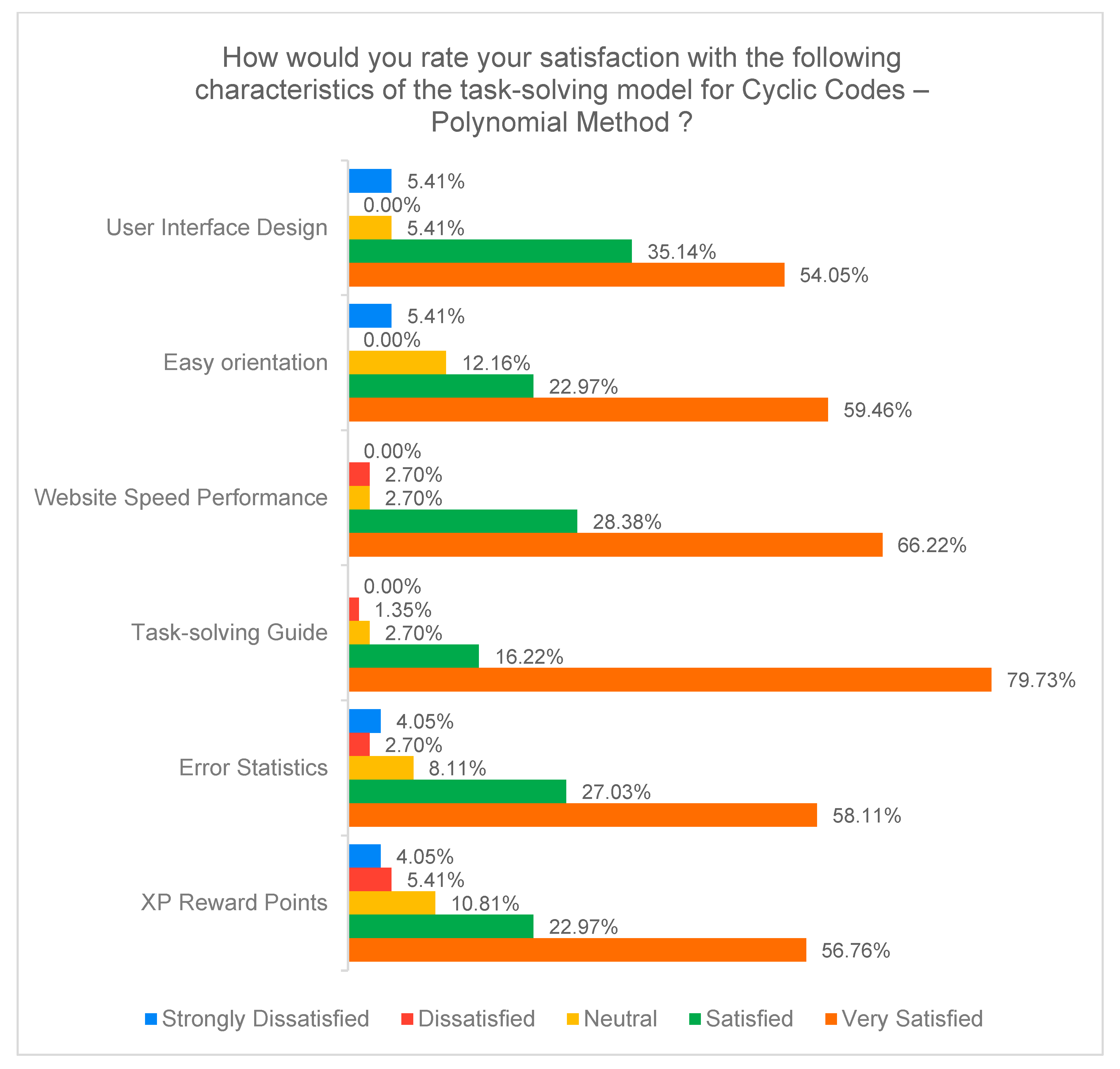
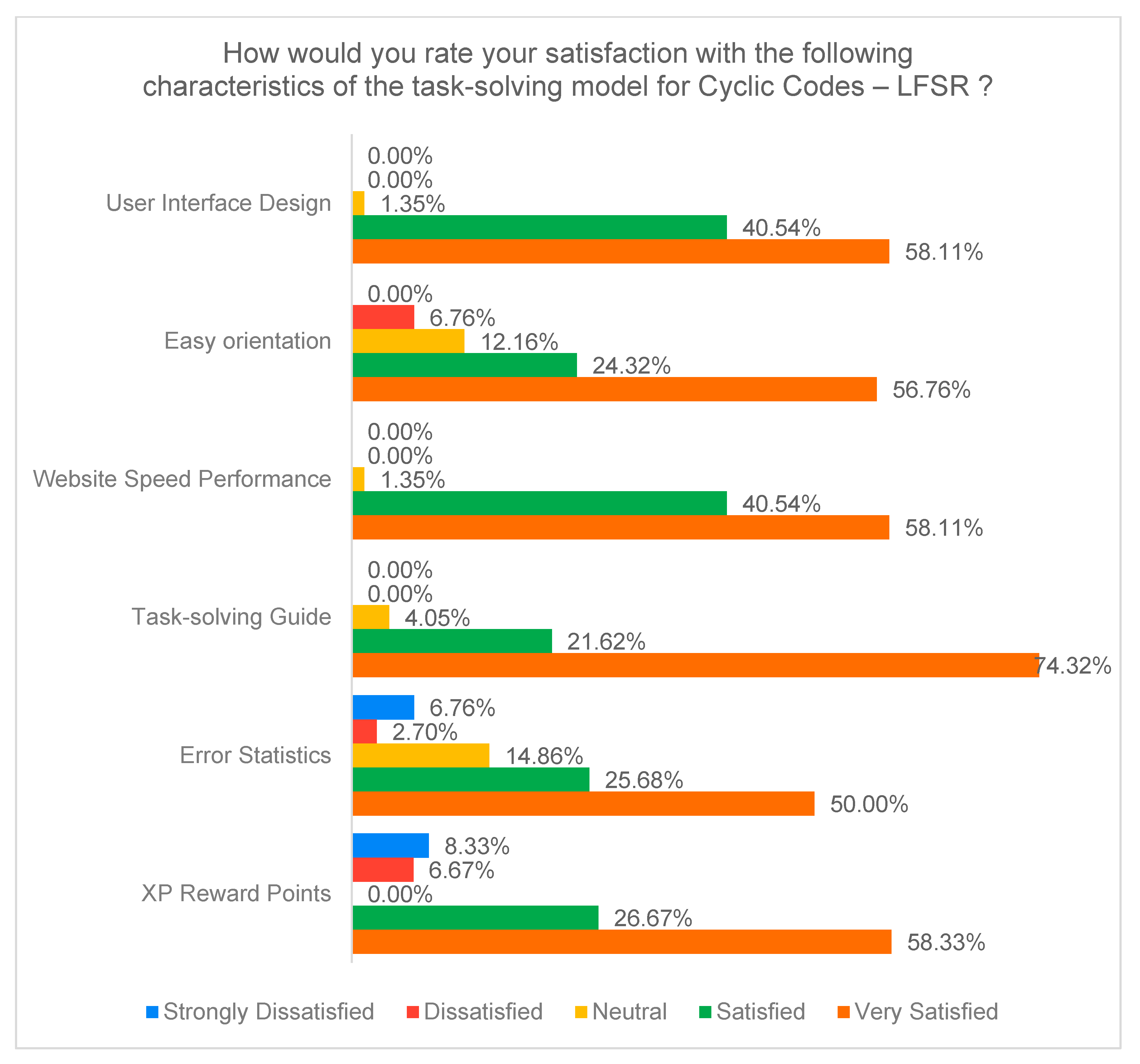
As part of the study, a survey was conducted to investigate the degree of student satisfaction with various features of the two interactive educational software tools developed to support learning on the topic of cyclic codes. The survey included 74 volunteer participants who rated each of the two models separately using a five-point Likert scale (“Strongly Dissatisfied”, “Dissatisfied”, “Neutral”, “Satisfied”, and “Very Satisfied”). The features evaluated covered key aspects of the user experience, including: “User Interface Design”, “Easy Orientation”, “Website Speed Performance”, “Task-solving Guide”, “Error Statistics”, and “XP Reward Points”.
The survey results for the first training model (polynomial method), given in
Figure 29, show a high overall satisfaction among the participants. Most features, including interface design, orientation, and site speed, were rated positively, with the responses “Satisfied” and “Very Satisfied” dominating. The highest satisfaction was reported for the task-solving guide, while the reward points element (XP Reward Points) received more moderate ratings, suggesting potential for improvement in this area.
The survey results for the second learning model (LFSR Method) in
Figure 30 also show high overall satisfaction among students. Most features, including interface design, orientation, and website speed, were rated primarily as “Satisfied” and “Very Satisfied.” The Problem-Solving Guide again stands out as the highest rated feature, while the “Error Statistics” and “XP Reward Points” features receive more mixed ratings, including some dissatisfaction, indicating room for improvement in these components.
Possible reasons for the lower and more mixed evaluations of the XP Reward Points and Error Statistics functionalities may be related to the way in which students perceive them. In the case of XP Reward Points, it is possible that some students do not see a direct connection with the acquisition of the learning content and perceive it as a game element, while others would expect a more flexible and motivating incentive system. Regarding Error Statistics, it is possible that for some students this feature is useful for self-reflection, but for others it is perceived as an unnecessary burden or an additional assessment element. These hypothetical reasons may explain the diversity in the feedback and indicate that there is potential for improvements aimed at emphasizing the pedagogical value and practical applicability of both functionalities.
