Abstract
The present study examines the application of interactive software models for training on the topic of “Cyclic Codes” in order to increase the success rate and engagement of students in technical disciplines. Two models have been developed—based on the polynomial method and the LFSR approach—through an established methodology adapted to the specifics of the content. A pedagogical experiment with a control and experimental group was conducted, and ANCOVA analysis was applied to eliminate the influence of initial grades. The results show a statistically significant advantage of the experimental group in terms of final grades, which confirms the positive effect of using interactive models. The analysis of engagement and solved tasks reveals that the polynomial model is used more widely and contributes to the systematic application of algorithmic steps, while the LFSR model has an illustrative nature and supports intuitive understanding through visualization of processes. The feedback received from students shows high satisfaction and points to improvements in the interface and functionality. In conclusion, interactive models prove their effectiveness as complementary tools for learning complex technical concepts, and prospects for future development through the integration of artificial intelligence and enhanced gamification are also discussed.
1. Introduction
In modern education, digital and interactive learning tools are emerging as key to increasing student engagement, motivation, and learning outcomes. The European Commission highlights the need for accessible and effective digital learning platforms [1], and the OECD (Organization for Economic Co-operation and Development) Digital Education Outlook 2023 shows that gamified and interactive solutions significantly improve the quality of learning [2]. These recommendations outline the context and justify the need for research on virtual labs and modern teaching methods.
Simulation-based learning software tools combine a number of features that make them particularly effective in the educational process. Three key aspects stand out: the activation of cognitive processes and motivation through gamification; the use of implicit scaffolding to guide learning without direct mentoring; and the role of automatic feedback and adaptive difficulty in supporting deep understanding and sustainable knowledge.
Empirical research shows that simulations, combined with elements of gamification, significantly enhance cognitive processes such as attention, memory, and problem-solving skills while simultaneously increasing student motivation and engagement [3,4,5].
The concept of implicit scaffolding is based on creating a learning environment—through affordances, cueing, and automatic feedback—to support learning without excessive guidance. In a simulation context, this allows students to engage with concepts through self-directed exploration [6].
Automatic feedback and adaptive difficulty in learning platforms have been shown to enhance understanding and retention, especially when integrated into interactive and gamified environments [7,8].
One notable example of a successful national virtual laboratory infrastructure is the Virtual Labs Initiative developed by the Ministry of Education in India. This platform offers over 100 online labs in various engineering disciplines, such as theoretical codification and communication systems, and serves over 20 million students, demonstrating the broad potential of web-based simulation environments as accessible and effective tools for technical learning [9]. This platform provides a web-based simulation of cyclic codes in which students can enter a binary message, use a cyclic code, and observe the results of encoding and decoding using an LFSR and a Meggitt decoder. This provides real-time learning with visual feedback and control of the correctness of the solutions. The disadvantage of this simulation system is that only one specific generator polynomial and a fixed number of four information bits can be used [10].
There are scientific studies that confirm the effectiveness of virtual laboratories through a meta-analysis of 46 experimental and previously published studies in engineering education, showing a statistically significant effect on academic performance (Hedges’ g = 0.686; Confidence Interval 0.414–0.959), with the highest values being reported for motivation (g = 3.571) and student engagement (g = 2.888) [11,12]. Similar studies confirm that virtual simulation environments do not replace traditional laboratories but significantly contribute to active learning and overcoming limited resources in the laboratory.
In the context of the growing importance of interactive simulation systems in engineering education, this study focuses on the design, development, and experimental investigation of software training models designed to support the teaching of cyclic codes. The developed models cover both the polynomial form and the implementation of a linear feedback shift register (LFSR) in cyclic codes. They are built on an adapted methodology for creating learning environments [13]. The models presented here are an integral part of the broader virtual laboratory for teaching coding theory, described in detail in a previous study by the authors [14], where the overall architecture of the system, pedagogical principles, as well as integrated modules for tracking learning activity and evaluating results are considered. In this article, attention is specifically focused on the cyclic code modules—their algorithmic design, program implementation, and pedagogical applicability—assessed through a series of experiments with students in a real learning environment.
Research [15] shows that combining virtual reality and gamification significantly enriches learning. A systematic review of 112 articles reveals that these environments support a variety of pedagogical approaches and increase motivation, engagement, and student outcomes, outperforming traditional learning. Thus, gamified virtual reality has been established as an effective educational tool that is applicable across all levels and disciplines.
Another study [16] analyzes the effect of implementing Digital Game-Based Learning (DGBL) combined with gamification on the academic performance and motivation of university students. In an experiment with 126 participants divided into a control and experimental group, significant improvements were reported in the performance of students in the experimental group, while motivation remained high for all participants. The results show that gamified DGBL is an effective tool for active learning that provides immediate feedback, increases academic performance, and maintains a high level of engagement.
The study in [17] examined the use of virtual labs (V Labs) in distance learning in cybersecurity and their impact on active learning and student engagement. A study among students and faculty at Blekinge Tekniska Högskola, Sweden, presented positive evaluations of the use of V Labs as a means of interactive and hands-on learning. The results indicated that virtual labs facilitate the understanding of key concepts, develop problem-solving skills, and are perceived as an effective tool for enhancing active participation in learning.
In the context of the COVID-19 pandemic, which has radically changed laboratory learning, Reference [18] demonstrated that even a low-cost virtual lab built on PowerPoint allows students to participate in interactive exercises, make choices, and receive immediate feedback. This approach significantly increases engagement and improves learning outcomes in microbiology education. The study also highlights the need for further development of embedded assessments, interactive features, and access to detailed analytics for educators to optimize the effectiveness of virtual labs.
The study in [19] conducted a systematic literature review focused on the integration of virtual laboratories in science education. The authors summarized existing research, examining different models of virtual laboratory implementation, their impact on student participation, understanding of scientific concepts, and the development of digital skills. The results showed that virtual laboratories significantly improve the learning process by increasing student motivation and engagement as well as by providing a safe and flexible environment for experimental work. The review also emphasizes the need to combine virtual and real laboratory exercises to achieve optimal educational outcomes.
The study in [20] conducts a systematic review of research related to interactive virtual laboratories using virtual reality (VR). The authors analyze various VR platforms and applications in science and engineering education, assessing their impact on student engagement, concept acquisition, and practical skills. The results show that interactive VR laboratories improve understanding of complex concepts through an immersive and engaging learning experience while providing a safe environment for experimentation. The review highlights the potential of VR technologies for developing innovative teaching methods but notes the need for further empirical research to assess the long-term effects on learning outcomes.
The study in [21] presents ARIS, an open platform for developing mobile learning experiences that allows the creation of interactive and personalized learning modules. The article examines the functionalities of the platform, including the ability to integrate multimedia elements, gamification, and the collection of data on the progress of learners. The results show that the use of ARIS can increase student engagement and facilitate adaptive learning through interactive scenarios that meet the individual needs of learners. The author emphasizes that the platform provides flexible capabilities for developing mobile learning applications, which makes it a valuable tool for modern educational practices.
Cyclic codes are a subset of linear codes characterized by the fact that the cyclic shift of one codeword leads to another valid codeword. This feature allows the use of polynomials and efficient algorithms in their processing [22]. They include important representatives, such as Hamming codes, BCH codes, Reed–Solomon codes, and their extended variants, which are used in the correction of single and double errors as well as packet errors.
Among the specialized types of cyclic codes, CRC (Cyclic Redundancy Check) codes stand out as the most widely used for error detection, especially in network protocols and storage systems. CRC codes are widely used in Ethernet, Wi-Fi, Bluetooth, file formats (ZIP), hard drives, SSD devices, and peripheral communication interfaces due to their high sensitivity to transmission errors and minimal computational load. They provide reliability in detecting single, double, and burst errors.
More recent research [23,24] demonstrates the potential of CRC codes not only as error detection tools but also as correction tools when combined with methods such as Guessing Random Additive Noise Decoding (GRAND). With such approaches, CRC codes, especially short and high-speed ones, can compete with, and in some cases even outperform, the effectiveness of BCH and Polar codes in some low-latency scenarios, making them attractive for IoT, URLLC, and other time-critical applications.
Due to their high reliability, low computational complexity, and easy software and hardware implementation, CRC codes are among the most widely used cyclic codes in practice. In the context of this article, the term cyclic codes will be used synonymously with CRC codes, since this particular class is the subject of design, simulation, and educational analysis. The presented models are based on polynomial form and LFSR-based coding and are intended for use in a virtual laboratory environment.
The aim of this investigation is to create two interactive models for learning cyclic codes and to conduct an experimental study to assess their pedagogical value and applicability in a virtual coding theory laboratory.
Although in recent years many interactive and virtual learning solutions have emerged to increase student motivation and engagement [15,16,17,18,19,20,21], there is a lack of models specifically focused on the teaching and learning of cyclic codes. Furthermore, the literature highlights a lack of a comprehensive approach that covers all stages—from design to development and implementation of interactive educational tools based on a common methodology. While empirical studies exist in other disciplines, they are usually limited to the application of a single method—surveys, tests, or analysis of results. In the context of CRC codes, systematic studies that combine pedagogical experiments with the application of statistical methods, analysis of system activity, and student surveys are absent. The present work addresses this gap through three independent studies, which together provide a more comprehensive and reliable picture of the effectiveness of the two proposed models in a virtual laboratory environment.
2. Materials and Methods
2.1. A Methodology for Designing and Developing an Interactive Software Model
The design and development of effective interactive learning software requires adherence to a clearly defined and systematic methodology. An approach based on sequential stages—from analysis of the learning content and objectives, through functional modeling and visual design, to testing and implementation—guarantees not only technical sustainability but also pedagogical effectiveness of the developed tool. According to [25], the use of structured development, based on established principles of multimedia learning, significantly increases knowledge acquisition and student engagement in an electronic environment. Especially in interactive solutions that combine simulations, visualization, and real-time feedback, adherence to a systematic software process helps to achieve coherence between learning goals and technical implementation.
This article presents an adapted version of the methodology for the design and development of software interactive tools (Figure 1), proposed in [13], where the creation of a Hamming code training model using the general algorithm is considered. The methodology encompasses a clearly structured sequence of stages—from theoretical analysis and formulation of an algorithmic scenario, through requirements definition, to programming, testing, and integration into a training environment. In the present work, it is adapted to the specifics of cyclic codes and the two approaches used (polynomial and linear feedback shift register). A detailed discussion of the general methodology is the subject of [13] and will not be presented here to avoid repetition and focus on the new programming and functional aspects of the models under consideration.
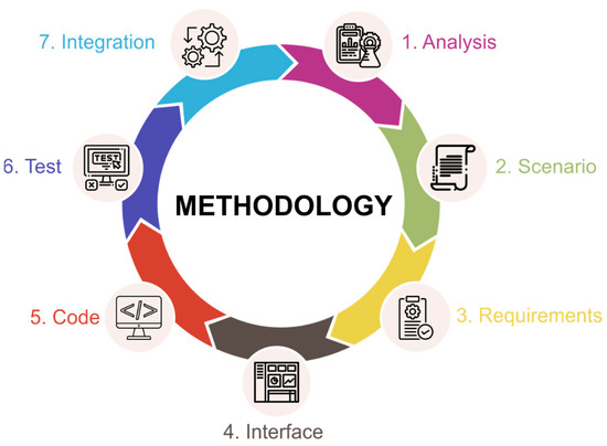
Figure 1.
Methodology for designing and developing an interactive software model [13].
The following sections of the article present some of the main phases of the application of the adapted methodology for the design and development of interactive software models aimed at training in cyclic codes. In particular, the emphasis is placed on Cyclic Redundancy Check (CRC) codes, which are implemented through operations with polynomials in the finite field GF(2). The specific solutions implemented in both approaches—through the polynomial method and through a linear feedback shift register (LFSR)—are examined. The emphasis is placed on the functional logic, visualization of the algorithms, and structuring of the user interaction, which follow the general methodological framework but are tailored to the specifics of the respective coding mechanism.
For greater clarity and systematic differentiation of the two interactive models, we have created a comparative table (Table 1). It summarizes their main characteristics according to several key criteria: algorithmic complexity, educational advantages, intuitiveness and analytical precision, and level of difficulty in implementation.

Table 1.
Comparative analysis of the two models for learning cyclic codes.
2.2. Designing an Interactive Software Model for Solving Problems with the Cyclic Code—Polynomial Method
The study of cyclic codes through their polynomial form has particular value in an educational context, as it allows for a deeper understanding of the principles involved in the calculation of check bits and error detection. By working with polynomials and operations modulo 2, students develop skills in tracing algorithmic steps, as well as the ability to analyze logical dependencies between the information and control parts of the codeword. This approach stimulates abstract thinking and builds analytical skills, which are essential in mastering the basics of digital communication and reliable information transmission.
2.2.1. Analysis of the Theoretical Foundations of a Cyclic Code by the Polynomial Method
Binary cyclic codes are an important subclass of linear block codes. Their core characteristic is that a resolved code combination is obtained again after shifting the bits of a resolved code combination [26].
When constructing the cyclic codes, it is accepted to represent the code combination by a polynomial to some variable, most often it is x,
where are coefficients taking values 1 or 0. For example, if (1) is applied to the binary combination 101001101, it will result as
There are several ways to construct cyclic codes using the polynomial method. One of the widely used ways of encoding is the so-called systematic form of representation in which the code combination polynomial F(x) has the following general form:
Here,
- -
- is a polynomial of the information combination whose degree is less than or equal to ;
- -
- is the remainder of the division of , where is a generator polynomial of degree , which must satisfy certain conditions;
- -
- —this product is equivalent to the binary left-shift operation of the information combination by positions, where, in effect, the degree of the polynomial is increased by .
A key point in encoding with a cyclic code is the choice of the generator polynomial , by which the noise immunity of the code is determined [27]. The criteria for choosing are as follows:
- -
- The power of must be equal to the number of control bits k;
- -
- The generator polynomial must be simple, irreducible, i.e., to be divisible without a remainder only by 1 and itself [26].
- -
- For a cyclic code with , the generator polynomial is formed as follows: . The polynomial must satisfy the previous two criteria. In this case, in practice, the control bits are incremented by one.
Table 2 gives a list of all primitive polynomials of degrees 1 to 10.
Table 2.
List of primitive polynomials of degree 1 to 10.
The rules for performing operations with polynomials used in cyclic codes and, in particular, in CRC are formulated within the finite field GF(2) and are summarized in Table 3.
Table 3.
Algebraic rules for polynomials.
The following example will be considered to illustrate the encoding process. For the information combination X = 1010101101, the polynomial cyclic code encoding must be performed using the above representation form.
The first necessary action is to define the code parameters, which in this case are as follows:
- -
- The number of information bits is ;
- -
- The number of errors the code can detect is
- -
- For the code, the Hamming distance is obtained;
- -
- For the number of check bits, the condition yields .
After the parameters of the code have been determined, a representation of the information combination in polynomial form follows. For this purpose, it is convenient to first write down the information combination as follows (Figure 2).
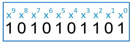
Figure 2.
Labeling the members of the information combination.
In the polynomial only those terms that have a value of 1 in the corresponding information combination are involved, as shown below:
The next step is an increase in the degree of the information polynomial to degree , which is achieved by multiplying by , as in the case .
Next, the generator polynomial is chosen. According to the conditions that were mentioned above and the polynomials from Table 2, a choice can be made between the two polynomials:
Let the polynomial be chosen.
The main operation in the task should also be performed, namely the division of the polynomials . The operation is shown in Figure 3.
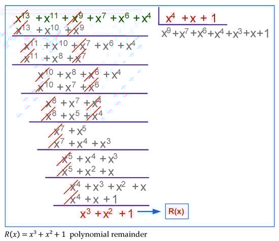
Figure 3.
Division of polynomials
As a result of the division, the polynomial remainder is obtained, which in practice determines the control bits:
After substituting in Formula (3) for the general form of the code combination , the following polynomial is obtained:
The last step is to convert the code combination from polynomial to binary form, replacing the missing terms in the polynomial with the value of 0.
2.2.2. Compilation of a Scenario for Solving Problems with Cyclic Codes by the Polynomial Method
Here, it is intended to solve tasks only in encoding mode. Figure 4 shows the general algorithm for solving a problem with this code.
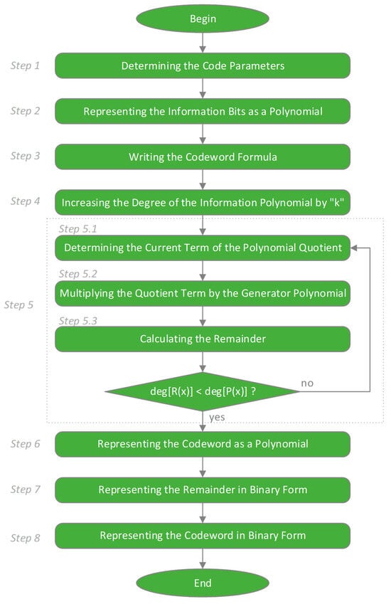
Figure 4.
Algorithm for solving problems with cyclic codes using the polynomial method.
The steps of the task-solving scenario are as follows:
- Step (1)
- Determining the Code Parameters. The parameters of the code— and , , —and the generator polynomial are determined.
- Step (2)
- Representing the Information Bits as a Polynomial. The information combination is converted from binary to polynomial form.
- Step (3)
- Writing the Codeword Formula. Formula (3) is written down.
- Step (4)
- Increasing the Degree of the Information Polynomial by “k”. Multiplication of the information polynomial by is performed, increasing the degree of the polynomial from to .
- Step (5)
- Performing the polynomial division . To more clearly present the actions of this step, the next few steps will demonstrate the first cycle of the example in Figure 3.
Step (5.1.) Determining the Current Term of the Polynomial Quotient. This action corresponds to the presented of Figure 5a moment of division, which in this case is the result of
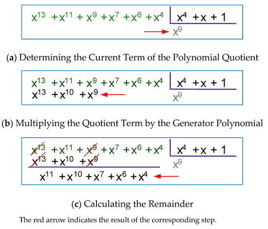
Figure 5.
First cycle of polynomial division
Step (5.2.) Multiplying the Quotient Term by the Generator Polynomial (Figure 5b). It is obtained as a result of the multiplication of the last term:
Step (5.3.) Calculating the Remainder (Figure 5c). It is obtained as a result of adding the result of Step 5.2 with the remainder of the previous cycle. If it is the first cycle, as it is now, add the result of Step 5.2 with the divisor :
Steps 5.1 to 5.3 are performed until the degree of the polynomial residue is less than the degree of the generator polynomial .
- Step (6)
- Representing the Codeword as a Polynomial. This action is expressed in the substitution in dependence (3).
- Step (7)
- Representing the Remainder in Binary Form. This is a conversion of the polynomial to binary format, with the missing terms replaced by the value of zero.
- Step (8)
- Representing the Codeword in Binary Form. This is a conversion of the polynomial to binary format.
2.2.3. Formulation of the Requirements to the Interactive Model for the Study of Cyclic Code—Polynomial Method
In addition to the general requirements for interactive models [14], the interactive software model for solving problems with a cyclic code using the polynomial method must also meet the following specific requirements:
- To be able to select a generator polynomial from a list of primitive polynomials in the control panel.
- To be able to write (record) the information combination in polynomial form .
- To be able to write the formula of the code combination .
- To be able to write the polynomial product
- To be able to perform the polynomial division .
2.2.4. User Interface Prototype
User Interface (UI) design is an important phase in the development of a software tool [28], and the need for specialized software tools for prototyping is key. These tools allow designers to quickly visualize ideas, test the user experience (UX), and collect feedback before launching expensive development. Especially when designing a web-based application for educational purposes, where clarity, intuitiveness, and efficiency of interaction are key to the educational process, prototyping helps to iteratively improve the design, ensuring that the application is easy to use and effectively reaches its target audience—students and teachers. Using such tools saves time and resources by identifying potential problems and user needs at an early stage. For the needs of this project, the Balsamiq Wireframes 4.7.5 tool was used, which simulates hand-drawn sketches [29].
The user interface prototype that was designed for the cyclic encoder model by the polynomial method is presented in Figure 6. At each stage of the task, where some polynomial needs to be entered, initially a field will be displayed with a series of question marks (“?????????”), which must be replaced with the corresponding expression (polynomial). As with previous models, all interface elements are planned to be grouped into four panels.
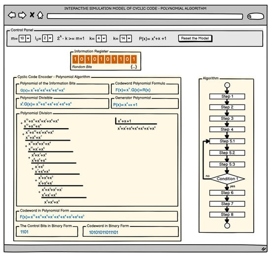
Figure 6.
User interface prototype of cyclic code research model—polynomial method.
Control panel. The difference in this panel compared to the Hamming model [13] is that an additional field has been added to specify the generator polynomial , provided that it can be selected from a preloaded list of primitive polynomials. The other difference is that there is no field to select the mode of operation, because this model will only work as an encoder.
Information register. It is similar to the information registers in the Hamming model [14], with the difference that there are numbers for more convenient conversion to polynomial form above the information bits instead of labels ().
Cyclic code encoder—polynomial algorithm. This is the block where the encoding process will take place. It consists of the following sections:
- -
- Polynomial of information bits. In this part, the conversion of the information bits to polynomial form will be performed.
- -
- Code combination formula. In this part of the encoder, the code combination formula will be written.
- -
- Polynomial of the divisor. This is the part of the problem where the result of the multiplication will be written.
- -
- Generator polynomial. This part will be filled automatically by the control panel.
- -
- Division of polynomials. This is the part of the encoder where the actual problem solution will be performed, namely the polynomial division . The division itself will be performed in iterations until a remainder with a degree less than the degree of the generator polynomial is obtained.
- -
- Code combination in polynomial form. This is the field where, after the remainder of the division is determined, the code combination polynomial according to the formula will be written.
- -
- Remainder in binary form. In this field, the conversion of the residual from polynomial to binary form will be performed.
- -
- Code combination in binary form. In this field, finally, the task will require converting the code combination from polynomial to binary form.
Algorithm. An interactive block diagram of the model operation algorithm based on that of Figure 4. By coloring the steps in different colors, it facilitates orientation while working with the model. When one points the mouse over a given step, brief information about the required action is displayed.
2.3. Designing an Interactive Software Model to Solve a Problem for Cyclic Codes via Linear Feedback Shift Registers
The use of a linear feedback shift register (LFSR) is an efficient and intuitive approach to implementing encoding and decoding for cyclic codes. The LFSR model simulates the behavior of a hardware register, where the input and output values are determined by sequential bitwise operations and feedback based on a given generator polynomial. This method not only facilitates the visualization of the algorithmic steps but also helps learners better understand the structure and logic of cyclic coding. Incorporating the LFSR into a training software model allows for the presentation of key concepts from coding theory through practical simulations that bring the abstract content closer to real hardware applications.
2.3.1. Analysis of the Theoretical Foundations of a Cyclic Code Using a Linear Feedback Shift Register
A characteristic of cyclic codes is that they can easily be implemented using a linear feedback (LF) shift register. It is known that the cyclic shifting of the polynomial of the code combination and the encoding of the polynomial of the information combination is conducted by dividing polynomials [26]. Such an operation can be performed by a scheme (linear feedback shift register, LFSR) for dividing polynomials, the general form of which is shown in Figure 7. Given two polynomials and , where
and
so that . The scheme of Figure 7 performs the steps of dividing the polynomial by , as a result of which the terms of the quotient and the remainder are determined:
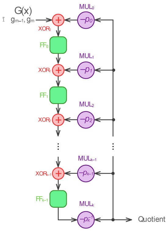
Figure 7.
General view of a polynomial division scheme [26].
Initially, the register is initialized with zero values. In the first shifts, the coefficients of are loaded in decreasing index order. After the -th shift, the coefficient of the output is , which is the term of the quotient with the highest index. For each coefficient of the quotient , the polynomial must be subtracted from the divisor. This is accomplished by feedback in the circuit of Figure 7. The differences between the leftmost terms, remaining in the dividend, and the terms of the LF are formed at each circuit shift and are obtained as a result in the register cells. Each time the register is shifted, the difference is shifted by one position. The highest-order term is shifted to the output while the next significant coefficient of is submitted to the input of the circuit. After a total of () register shifts, the coefficients of the quotient will successively be output, and the coefficients of the remainder will be obtained in the register cell.
- Systematic encoding with -bit linear feedback shift register.
Cycle code encoding in systematic form (discussed in Section 2.2.1) involves computing the control bits as the result of the shift and divide operations (). The shifting is necessary to make space for the control bits, which are added to the information bits and thus form the code combination vector. Shifting the information bits by positions is a trivial operation and, in practice, is not performed by the division circuit; instead, only the control bits are calculated then placed in the appropriate place in the code combination. The control bit polynomial is obtained as the remainder of the division , which in practice is obtained as the result in the cells of the -bit linear feedback shift register shown in Figure 8. The elements marked with () represent adders modulo 2. The combinations of LF correspond to the coefficients of the generator polynomial , which is written as follows:
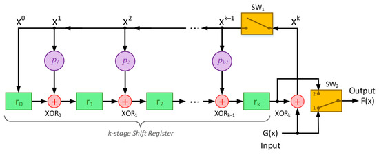
Figure 8.
Encoding using a -bit linear feedback shift register.
The following steps describe the encoding process using the circuit of Figure 8.
- (1)
- Switch 1 (SW1) is closed during the first shifts (—number of data bits) to allow data bits to pass through the -bit shift register.
- (2)
- Switch 2 (SW2) is in position 1 during the first shifts in order to allow information bits to be directly written to the output register (code combination register).
- (3)
- After passing the -th bit of the information combination, Switch 1 is opened, and Switch 2 is switched to position 2.
- (4)
- The remaining shifts clear the register by shifting the control bits from the register cells into the output register.
- (5)
- The total number of shifts is equal to and the output register is filled with the bits of the code combination ().
Figure 9 shows the steps of calculating the control bits and forming the code combination using a 4-bit linear feedback shift register based on the polynomial . In steps 1 to 8, the control bits are formed, and in step 9, the control bits are shifted to the output of the circuit.
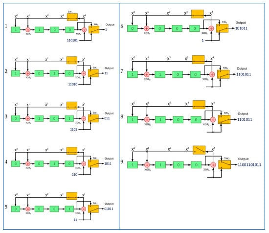
Figure 9.
Encoding stages of an information combination with in a cyclic code by means of a -bit linear feedback shift register based on the polynomial
2.3.2. Writing a Scenario to Solve Problems for “Cyclic Codes via Linear Feedback Shift Registers”
With this type of cyclic code, it is also only intended to solve problems in encoding mode, as was the case with the polynomial method. Figure 10 shows the general algorithm for solving problems with a cyclic code using a linear feedback shift register. The encoder of Figure 8 will be used as the basis of the interactive model, and the model will also include two registers, for the information bits and for the code combination, respectively.
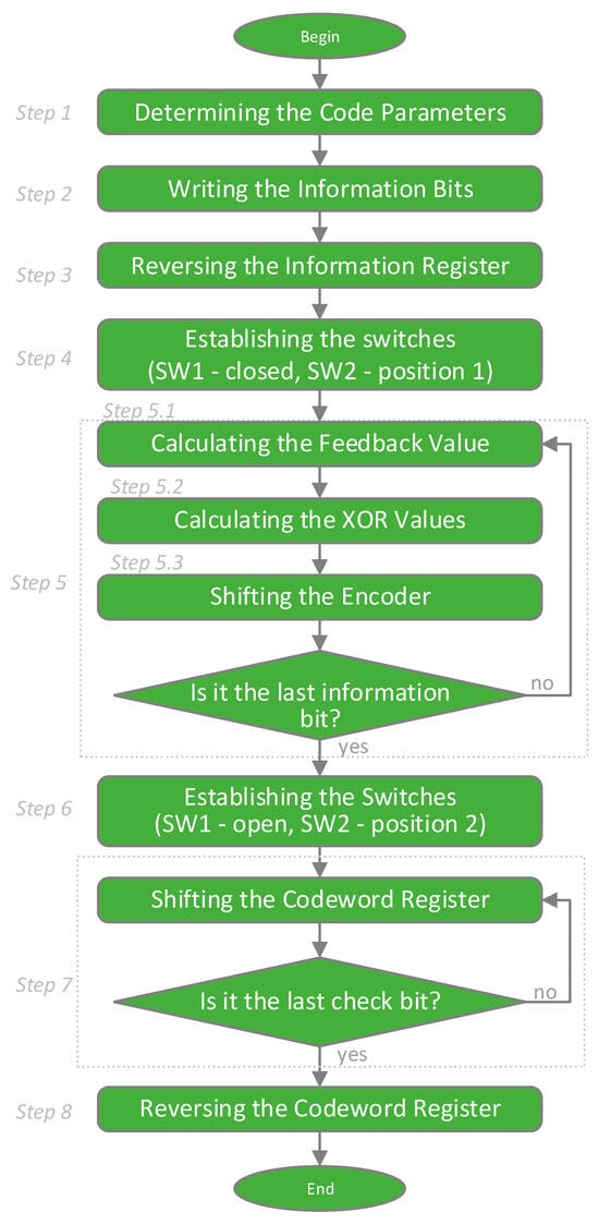
Figure 10.
An algorithm for solving problems with cyclic codes by linear feedback shift registers.
The steps of the task solving scenario are as follows:
- Step (1)
- Determining the Code Parameters. The parameters of the code are determined— and , , and the generator polynomial
- Step (2)
- Writing the Information Bits. The information combination is set in binary form in the information register.
- Step (3)
- Reversing the Information Register. This represents shifting the bits of the register so that the first bit becomes last, the second bit penultimate, and so on. This step is artificially added to make the final result match that of the polynomial method. The difference in results is due to the fact that the generator polynomial of the shift-register encoder is written in increasing power order from left to right, while in the other method, it is the other way around.
- Step (4)
- Establishing the Switches. During the first iterations, switch must be in closed position and switch must be in position 1.
- Step (5)
- Calculation of Control Bits. This step will run in iterations. After the end of the -th iteration, the final control bits will be received in the bits of the shift register. Each iteration includes the following stages:
Step (5.1) Calculating the Feedback Value. This action is taken by calculating the value of the adder .
Step (5.2) Calculating the XOR Values. In this substep, all elements are calculated except for the last one, which is responsible for the feedback.
Step (5.3) Shifting the Encoder. This is achieved through the following steps:
- -
- The value of the feedback is recorded in the first cell of the register;
- -
- The values of the elements are written in the corresponding bits (cells) of the register;
- -
- The data register is shifted one position to the right, moving the bit out of the register into the output register, i.e., the code combination register.
- Step (6)
- Establishing the Switches. After iterations switch should be established in open position, and switch in position 2.
- Step (7)
- Shifting the Codeword Register. In this step, the control bits received in the bits of the shift register are shifted into the code combination register. The move is made bit by bit in iterations.
- Step (8)
- Reversing the Codeword Register. This step is analogous to Step 3 with the information register. The purpose of this step is the same, i.e., to match the results of the two methods.
2.3.3. Formulation of the Requirements of the Interactive Model for the Study of a Cyclic Code Using a Linear Feedback Shift Register
The following requirements, in addition to those of Section 2.3.2, can be formulated for this interactive software model for solving tasks for encoding with a cyclic code using a linear feedback shift register:
- (1)
- To be able to select a generator polynomial from a list of primitive polynomials in the control panel.
- (2)
- The information combination register should have additional functionality to reverse its values.
- (3)
- The code combination register should only have the value reversal and right shift functionalities.
- (4)
- On the basis of the selected generator, polynomial should be able to recreate the structure of a linear feedback shift register by analogy with that of Figure 8. Its input should receive the bits from the information register, and its output should output the values to the code combination register.
- (5)
- Switches and should be interactive, changing positions when clicked, and should initially be in neutral positions.
- (6)
- All elements should be interactive, changing their values from 0 to 1 and vice versa when clicked.
- (7)
- Linear feedback -bit register should have the functionality to shift right by one position.
2.3.4. User Interface Prototype
The user interface prototype that was designed for the cyclic encoder model implemented by a linear feedback shift register with generator polynomial is presented in Figure 11. In the proposed graphic layout, the interface elements are grouped into five panels.
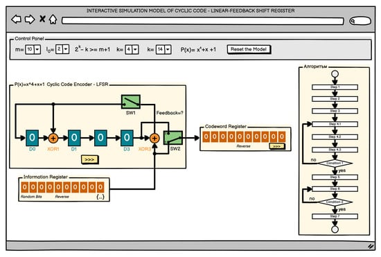
Figure 11.
User interface prototype of the programming model for exploring a cyclic code by a linear feedback shift register with the generator polynomial
Control panel. It has the same appearance and functionality as the cyclic encoder by the polynomial method of Figure 6.
Information register. It is similar to the previous information bits but with an additional “Flip” functionality whereby the register bits are mirrored.
Encoder of cyclic code—linear feedback shift register. This is the main panel where the control bits will be calculated. It is based on the register of Figure 8. The interactive elements in this panel are the two switches SW1 and SW2, which will change positions when clicked; the sum modulo 2 elements XOR1 and XOR3, which will change values on click; and shift button “>>>”, through which the register bits will be loaded.
Code combination register. This register will serve to store the code combination, which will be formed step by step in the process of the work. Two functional buttons are associated with it—“Invert” and shift the bits by one position to the right “>>>”.
Algorithm. Interactive block diagram of the algorithm of working with the model based on that of Figure 10. By coloring the steps in different colors, it facilitates orientation while working with the model. When one points the mouse over a given step, brief information about the required action is displayed.
2.4. Program Design and Component Structure of the Two Interactive Tools for Cyclic Codes
This section presents the program design and component structure of the two developed interactive software tools for solving problems using cyclic codes. The first tool uses a polynomial method based on division modulo 2 with a generator polynomial, and the second—a linear feedback shift register model, implementing the same process by simulating a hardware register. The two software models use a common methodology but have different internal logic, visualization, and interaction methods. The section describes the technologies and program libraries used, as well as basic UML diagrams illustrating the structure and interaction between the functional components of the system. The aim is to emphasize the modularity, reuse, and upgradeability of the developed educational tools.
2.4.1. Programming Languages and Libraries Used
In the implementation of both software models, web-based technological tools were used, which allow for wider access and compatibility with different devices and operating systems. The main programming language is JavaScript (ES2024) [30], which manages the logic of interaction and the visualization of the algorithms. HTML5 and CSS [31,32] are used to implement the user interface and graphic layout. For more effective management and manipulation of DOM (Document Object Model) elements of the page and event processing, the jQuery library [33] is used. The Konva library [34] is used to implement interactive two-dimensional graphics, representing the actual actions of the processes of solving problems using cyclic codes.
For storage and management of data related to user work, server logic has been implemented using the PHP language [35] and the MySQL database [36]. Each solved example is registered in real time with the necessary statistical data in the system database. The functionality implemented in this way allows the accumulation of detailed statistical information, useful both for pedagogical analyzes and for adapting the learning strategy according to the individual progress of each learner.
UML (Unified Modeling Language) diagrams are an established standard for visual modeling of software systems [37]. They facilitate the understanding, design and documentation of the functionality and structure of program components. Two main diagrams were used in the design of interactive models: an activity diagram, which shows the sequence of actions when solving tasks, and an object diagram, which reflects the state and interaction between specific program objects. These visualizations support not only the implementation, but also the future development and adaptation of the software tool.
In the JavaScript language, it is more correct to use an Object diagram instead of a Class diagram, because objects are created directly and inheritance is carried out through a prototype chain, unlike classical languages such as Java and C++, which use the traditional class model for inheritance and object creation.
In designing the two software models for studying cyclic codes, a common framework of an interactive software model was used, which is presented in Figure 12 through an object diagram. This model was also used in the design of the other models of the virtual laboratory on coding theory [14].
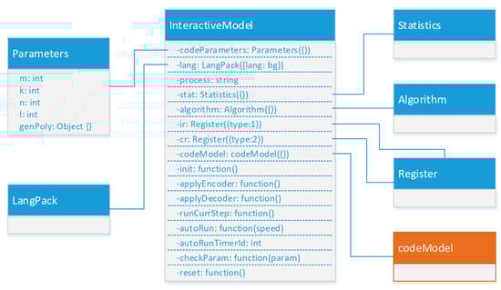
Figure 12.
Generalized object diagram of the interactive model.
The components (objects) in the diagram in Figure 12 have the following main purposes:
- InteractiveModel—a main object that serves to connect, coordinate, and manage all other components;
- Parameters—an object that serves to store the code parameters;
- LangPack—an object that serves to store the labels and phrases for translating the user interface (currently there are translations into Bulgarian and English);
- Statistics—an object for storing temporary statistical data from solving the task and registering them in the database at the end of the task;
- Algorithm—an auxiliary object for visualizing the steps in solving the task using the interactive model;
- Register—an object for entering and storing the information bits and bits of the code combination;
- codeModel—a general component that provides functionalities necessary for studying different types of codes. In the following points, this component will be considered in the cases of cyclic codes using the polynomial methods and when using a linear feedback shift register.
2.4.2. Program Design of the Interactive Software Model for Studying Cyclic Code Using the Polynomial Method
Figure 13 shows the object diagram of the polynomial method cyclic code model, which is represented in Figure 12 by the name codeModel.
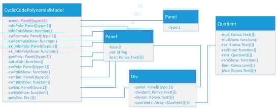
Figure 13.
Object diagram of the software model for studying the cyclic codes using the polynomial method.
From the diagram in Figure 13, it can be seen that the code model uses one main object called “CyclicCodePolynomialModel” and several auxiliary objects such as “Panel” (type 1 and type 2), “Div”, and “Quotient”. Some of the main functionalities of the “CyclicCodePolynomialModel” object are entering the polynomial of the information bits, performing the action , entering the codeword formula, a method for automatic solution of the problem by visualizing the individual steps, etc. The “Div” object serves to implement the cyclic polynomial division . It, in turn, uses an array of objects of type “Quotient” to store the intermediate results of the division.
The process of solving a problem using the interactive software model for studying cyclic codes is shown in Figure 14 through an activity diagram. In this diagram, the conditional element “Check the condition deg[R(x)] < deg[P(x)]” checks whether the degree of the polynomial R(x) is less than the degree of the polynomial P(x).
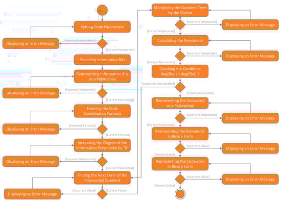
Figure 14.
Activity diagram for the cyclic code model using the polynomial method.
2.4.3. Program Design of the Interactive Software Model for Studying Cyclic Codes via Linear Feedback Shift Registers
Figure 15 shows the object diagram of the cyclic encoder model (represented by codeModel in Figure 12), based on a linear feedback shift register, presenting some of the most important objects and functions included in its composition. It can be seen that several additional objects have been developed for the purposes of the model:
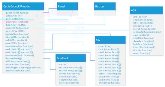
Figure 15.
Object diagram of the software model for studying the cyclic code via linear feedback shift register.
- Interactive switch “SW”, in two varieties—open/closed type (SW1) and a two-position variant (SW2)—which switches its position to the opposite state when the mouse is clicked.
- Adder mod 2 “XOR”. Depending on the type of the generator polynomial, the number of instances of this component in the model is different. The interactivity of the component is expressed in the fact that when the mouse is clicked, it takes on a value of 0 or 1, and with each click, the value is inverted.
- “Feedback”. This object serves to store and visualize the current value of the feedback at each stage of solving the problem, with its necessary functions.
The actions in solving a task using the software model for studying a cyclic code based on a linear feedback shift register are shown in Figure 16 through the activity diagram.
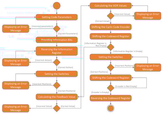
Figure 16.
Activity diagram for the cyclic code model via a linear feedback shift register.
3. Results
3.1. Implementation of a Software Training Model for Learning Cyclic Codes
This part of the article presents the final result of the implementation of the training software tools for learning cyclic codes, developed based on the adapted methodology and according to the formulated requirements and previously proposed prototype designs. The next two subsections present the developed training models, with the emphasis on the visualization of the final implementation. The details regarding the design and functional logic are not considered in depth, since they were already presented in the previous stages of the design process.
3.1.1. Model for Learning Cyclic Codes by the Polynomial Method
Figure 17 presents the graphical user interface of the implemented model for learning cyclic codes using the polynomial method. At this stage, the model can solve tasks related only to the encoding process, and at a later stage, functionality will be added for the decoding process. The developed model supports learners through a visual environment with step-by-step execution, automatic checking, and interactive feedback. The specifics of the solution are as close as possible to the manual approach, which is the main conceptual idea underlying the model design.
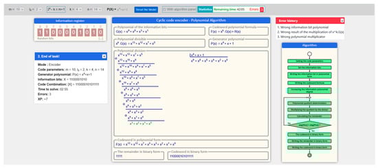
Figure 17.
User interface of the software model for studying the cyclic codes using the polynomial method.
One of the key points in solving problems related to cyclic codes is the correct choice of a generator polynomial. In the implemented model, this step is performed by selecting from a predefined list of admissible polynomials. Despite the provided help functionality, the student should be familiar with the basic rules that the appropriate generator polynomial must meet according to the condition of the problem. Figure 18 presents the interface for selecting a generator polynomial. The choice of a generator polynomial is limited by the parameters of the model with which it can be used.
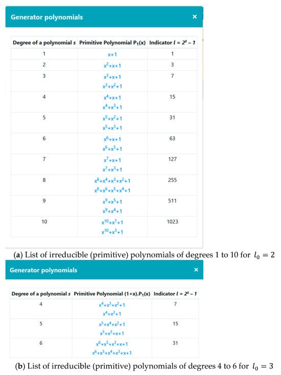
Figure 18.
Selection of a Generator Polynomial
The main form of interaction with the interactive model when solving problems on cyclic codes using the polynomial method is the introduction of a polynomial, which is input information for the coding or verification algorithms. In the context of a web environment, this process is not trivial, as it requires compliance with a specific syntax and validation against the mathematical structure of the polynomials used. To facilitate and accelerate this stage, a specialized function for interactive polynomial entry and verification has been implemented in the developed model, one which automatically analyzes the form and admissibility of the entered expression. Figure 19 shows the process of entering a polynomial both with correct and incorrect input, depending on the context of the current step in the algorithm, which supports the learner through immediate visual and text feedback.
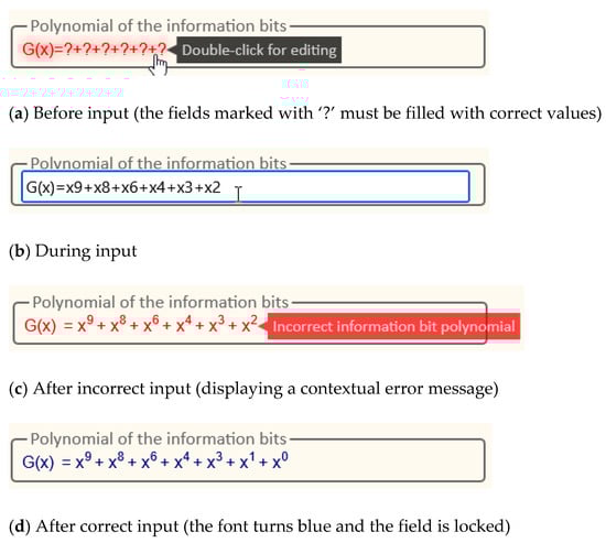
Figure 19.
Polynomial input process.
The main stage in solving a problem with the developed model is the execution of a polynomial division algorithm, in which the operation is implemented, according to the specifics of cyclic codes. For greater clarity and pedagogical efficiency, the division is organized into four repeated substeps which are performed cyclically until a remainder with a degree less than the degree of the generator polynomial is reached. Figure 20 shows a visualization of each of these substeps, including moving the divisor, applying bitwise operations modulo 2, and updating the current remainder, which allows the learner to follow the logic of the algorithm in real time.
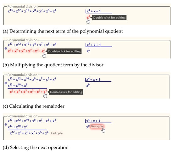
Figure 20.
Performing the first cycle of the polynomial division.
3.1.2. Model for Learning Cyclic Codes via Linear Feedback Shift Registers
Figure 21 shows the graphical user interface of the second implemented training model, designed to illustrate cyclic (CRC) encoding based on a linear feedback shift register (LFSR). This approach is closer to the hardware implementation of the algorithm and aims to familiarize learners with the way the code is implemented in a machine environment. The model allows tracking the encoding process by simulating the states in the registers, visualizing the bit stream, and dynamically updating the values in each clock cycle, according to the algorithm in Figure 10. The model, as with the previous one, supports step-by-step execution and automatic error detection, which helps to understand the principle of operation of the LFSR in close to real-world conditions.
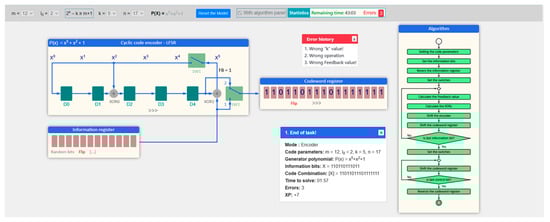
Figure 21.
User interface of the software model for studying the cyclic codes via linear feedback shift registers.
Interaction with the model in Figure 21 is carried out entirely through graphical elements, without the need to enter data from the keyboard. This facilitates practical work and draws attention to the logic of the algorithm. The LFSR configuration and feedback positions are automatically created based on the selected generator polynomial, eliminating the need for manual tuning. The main actions that the learner performs are reduced to logical operations by selecting simulated XOR elements and controlled bitwise shifting of register values, carried out by sequential mouse actions. Thus, the model provides a controlled environment for experimenting with the algorithm, combining visualization of hardware behavior with active user participation.
3.2. Comprehensive Evaluation of the Educational Impact of the Interactive Learning Models
Evaluating the educational impact of the developed interactive software models is a key point in determining their applicability and usefulness in the learning process. In the context of error correction codes, characterized by high theoretical abstraction and algorithmic complexity, such as cyclic codes, it is important to check whether the use of interactive tools facilitates the understanding of basic concepts and supports the mastery of specific coding principles. The evaluation aims to examine the extent to which the developed models facilitate the learning process and increase student engagement. In addition, it includes a review of the usability of the interface, compliance with the previously set learning objectives, and subjective impressions of users regarding the effectiveness of the model. Such an evaluation could serve as a basis for identifying opportunities for improvement and for adapting the models to different learning contexts.
For the overall assessment of the educational impact of interactive learning models, it is purposeful to conduct a combined study of academic success, engagement, and satisfaction of students. The graphical representation of the experimental design is shown in Figure 22.
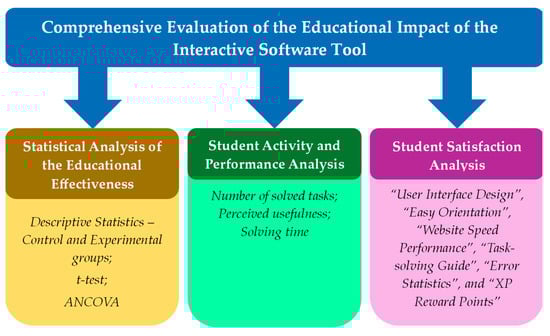
Figure 22.
Experimental design for the software tool.
3.2.1. Statistical Analysis of the Educational Effectiveness
Cyclic codes are studied within the course “Reliability and Security of Computer Systems”, taught in the third year of the Computer Systems and Technologies major at the University of Ruse “Angel Kanchev”. The developed interactive software model for studying cyclic codes using the polynomial method was implemented in the educational process in 2021 and is actively used at the time of writing this article as an alternative to the traditional written approach to solving problems. The second software model, based on a linear feedback shift register, was also introduced in 2021, but it serves primarily a demonstrative function, as it presents a new approach that has not been applied in the form of written exercises.
Conducting a pre-test as a way of establishing the initial academic level in the present study was not possible due to the specifics of the study, namely the formation of groups from different academic periods. This approach was necessary to comply with the principle of equality between students within the same cohort during the learning process. It is important to note that the idea of forming a control and experimental group arose only at the stage of implementing the interactive models. This means that during the training of the students from the control group, their participation in an experimental study was not foreseen, and their results were included post hoc. To avoid creating inequality within the same cohort, the experimental group was formed in a subsequent academic period, while the control group covered an earlier cohort. Although the groups are from different academic years, they are part of the same educational program, have gone through the same curriculum with the same teachers, and are educated under comparable institutional conditions.
Conducting a pretest as a way to establish the initial academic level in this particular case is not possible due to the specific conditions of the study, namely the formation of groups from different academic periods. This approach is required in order to comply with the principle of equality between students from the same stream during the educational process.
Within the framework of this study, the initial academic level of the participants was assessed by using the average grade point from the previous two semesters as an alternative to a pretest. Although this indicator does not directly measure knowledge on a specific topic, it provides a reasonable idea of the general academic level of the students. This allows for assessing the preliminary comparability between the groups and controlling for the possible effect of initial differences in preparation when interpreting the results after training. The choice to use grades from the last two semesters as an indicator of the initial academic level assumes that this period reflects the current state of student success and ensures sufficient completeness and comparison of data for all participants in the study. The data on the average grade were extracted from the examination protocols provided by the faculty office of the university.
To measure the final state of the participants in the study, the results of control papers (tests) on the topic of cyclic codes by the polynomial method, conducted by the training format of each of the groups, were used. Students from the control group conducted control papers in traditional written form, while participants from the experimental group used the interactive software tool, in the “Test” mode. In this mode of working with a model, restrictions have been introduced aimed at simulating conditions comparable to those of the written form—including a limited number of attempts to start a task and the impossibility of re-executing the model in case of an error. In this way, it is assumed that comparability, control, and objectivity are ensured in the assessment of the two groups, regardless of the differences in the teaching method used. The collection of data from the control works was carried out with the assistance of the teachers who taught the course. The tasks on cyclic codes with a linear feedback shift register are not included in this study, because they have no analogue in the control group, i.e., they were not studied in written form.
Before conducting comparative tests for the initial and final state, it is necessary to present information about the samples from both groups through descriptive statistics and frequency distribution. This allows for assessing the distribution of the results, detecting possible deviations or extreme values, and ensuring that the groups are comparable. For the statistical processing, the specialized software product SPSS v26 was used, which has found wide application in scientific fields when performing various types of statistical analyzes [38].
- Summary Statistical Data for the Groups in the Initial State
The number of participants in the control group is 91 students (from 2019 to 2020), and in the experimental group—102 students (from 2021 to 2025). The results of the descriptive statistics for the two groups at baseline are given in Table 4, and Figure 23 also shows the frequency distribution of the grades from the previous two semesters by group.
Table 4.
Descriptive Statistics of the Initial Academic Level of Participants.
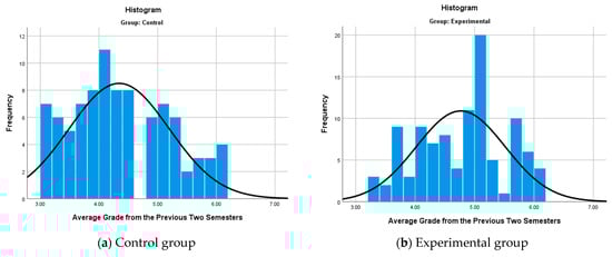
Figure 23.
Histogram of the distribution of the average grades from the previous two semesters.
- Statistical Comparison of the Initial State Between the Two Groups
At this stage of the study, a statistical test is performed to determine whether there is a significant difference in the average grade of the two groups at the beginning of the experiment, in order to determine whether the students were at a similar academic level before the application of the software models. The comparison of the overall academic level between the control and experimental groups was done through hypothesis testing, following the general algorithm shown in Figure 24.
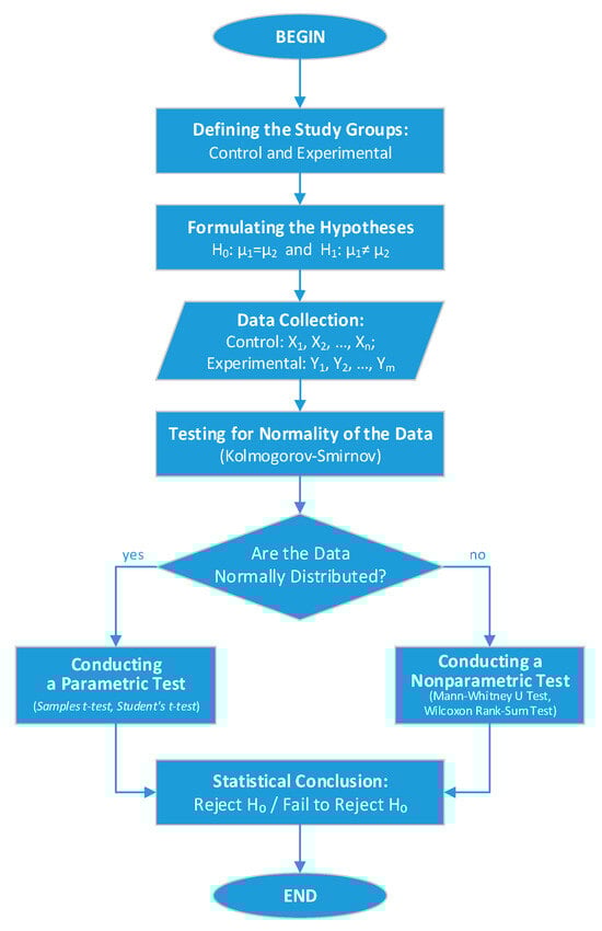
Figure 24.
General algorithm for hypothesis testing and election of an appropriate statistical test.
- -
- Formulation of the hypotheses and .
- The following two hypotheses are formulated:
- ○
- Null hypothesis —There is no statistically significant difference;
- ○
- Alternative hypothesis —There is a statistically significant difference.
- -
- Determination of the risk of error α
The risk of error or significance level (α) represents the probability of rejecting the null hypothesis when it is actually true. This value is determined in advance by the researcher and is used as a criterion for statistical significance. In practice, the most commonly used values for α are 0.05 or 0.01, which corresponds to a 5% or 1% acceptable risk when deciding to reject the null hypothesis [39]. In this study, a significance level of α = 0.05 was adopted.
- -
- Test Selection
The choice of an appropriate test for comparison depends on whether the data in the two groups are normally distributed. In this regard, a check for normality of the data distribution was performed using the Kolmogorov–Smirnov test, which is one of the widely used methods for assessing the correspondence between the empirical distribution of sample data and the theoretical normal distribution. The test compares the cumulative empirical function with the expected cumulative function under the normal hypothesis and allows one to assess whether the deviations are statistically significant [40]. The results of the normal distribution test are given for the control group in Table 5 and for the experimental group in Table 6, respectively.
Table 5.
Results of the Kolmogorov–Smirnov test for normal distribution for the control group at baseline.
Table 6.
Results of the Kolmogorov–Smirnov test for normal distribution for the experimental group at baseline.
According to the results obtained from Table 5 for the control group, it can be seen that the p-value (Asymp. Sig. 2-tailed) = 0.0798 is greater than the significance level α = 0.05. This means that there is not enough statistical evidence to reject the hypothesis of normal distribution, i.e., it is assumed that the data are normally distributed. The situation is similar for the experimental group (Table 6), where the p-value (Asymp. Sig. 2-tailed) = 0.089 is greater than the significance level α = 0.05. After it has been established that the data in both groups follow a normal distribution, according to the algorithm in Figure 24, a parametric test should be conducted for a statistical comparison of the mean values between the control and experimental groups.
An independent samples t-test for two samples (also known as Student’s t-test) was chosen, which is a classic method for assessing whether the difference between two means is statistically significant. The results of the t-test are given in Table 7.
Table 7.
Results of the t-test for the initial state of the control and experimental groups.
According to the results of Table 7, it was found that the p-value (Sig. 2-tailed) = 0.000 is less than the significance level ; therefore, the hypothesis is accepted, which states that there is a statistically significant difference in the average grades of the control and experimental groups. This suggests that the students from the control group had better academic achievements before the start of the experimental study. In such a situation, it is methodologically incorrect to make a direct comparison of the final results, since the reported differences could be due not only to the training method used, but also to the prior academic preparation of the participants.
The presence of a statistically significant difference in the initial academic level between the groups necessitates the use of a statistical control method, such as ANCOVA, in order to guarantee objectivity in the interpretation of the training results and to assess the real impact of the software tool used on academic success. The ANCOVA method allows for adjusting the final results so that the comparison between groups considers the initial differences and reflects the effect of the applied training approach.
- ANCOVA Analysis of Group Performance
ANCOVA (analysis of covariance) is a statistical method that allows for assessing the effect of an independent variable on a dependent variable, while simultaneously controlling for the influence of external factors (covariates) [41]. In the context of the present study, the method is suitable for assessing the impact of the software tool on the academic performance of students (results of control work on cyclic codes), taking into account their previous average grade. This provides a correction for the initial differences between the groups and allows for a more objective assessment of the effectiveness of the used training approach compared to the traditional method.
Within the framework of the analysis, the following variables are included in the ANCOVA model:
- -
- Dependent variable—the assessment from the control work on cyclic codes;
- -
- Independent variable—the group, i.e., the training method used (traditional or software);
- -
- Covariate variable—Average grade from the previous two semesters.
Before applying ANCOVA, it is necessary to check the homogeneity of variances between groups—one of the main assumptions for the validity of the analysis [41]. Violating it can lead to inaccurate results. For this purpose, the Levene test is used, which assesses whether the variations of the dependent variable are approximately equal in the compared groups. The results of the Levene test are given in Table 8.
Table 8.
Results of the Levene’s test for equality of variances for groups.
The results of the Levene test (Table 8) for homogeneity of groups show that the p-value (Sig.) = 0.233 is greater than the selected significance level α = 0.05. It follows that the assumption of homogeneity of variances is met, and the ANCOVA test can be continued.
The following general interpretation of the results of the ANCOVA test (Table 9) can be made:
Table 9.
Results of the ANCOVA analysis.
- -
- Corrected Model. This parameter represents the overall characteristics of the ANCOVA model. The obtained results F = 45.143, p (Sig) = 0.000 < 0.001 < α = 0.05 show that the model is statistically significant. This means that the included predictors (AverageGrade and Group) explain a significant part of the variation in the test results (Cyclic Code Test Scores).
- -
- AverageGrade. It expresses the influence of the covariance effect or in the current case the influence of the initial academic level (grade point average of the previous two semesters). With a result of F = 67.884 and p (Sig) = 0.000 < 0.001 < α = 0.05, which means that the grade point average has a highly significant influence on the results.
- -
- Group. The effect of the factor “Group” (reflecting the teaching methodology) is also statistically significant: F(1.190) = 6.061, p = 0.015 < α = 0.05. This means that the teaching method has an impact on the test results, even when controlling for the influence of the average grade from the previous two semesters.
In order to determine the effect of the factor “Group” more precisely, it is necessary to analyze the adjusted means of the dependent variable (cyclic code test scores) for each group, after controlling for the effect of the covariate (average grade). SPSS provides the ability to automatically output these values. Table 10 and Figure 25, respectively, present in tabular and graphical form the expected average values of the results of the control work on cyclic codes for the two groups, after accounting for the influence of the average grade from the previous two semesters.
Table 10.
Estimated marginal means of cyclic code test scores.
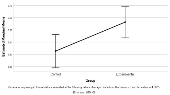
Figure 25.
Estimated marginal means of cyclic code test scores.
According to the results in Table 10, the value of the covariance (the average grade of the previous two semesters) is fixed at 4.5675 so that the two groups are compared at the same level of academic success. Under these conditions, the adjusted average value of the test scores for the experimental group is 5.564, which is 0.237 more than the control group. Although the difference seems small, it is statistically significant (p = 0.015), as confirmed by the results in Table 9, which indicates that it is not random.
The results of the analysis show that the use of software models in teaching, although leading to a relatively small increase in scores, has a positive effect on the assimilation of the learning material. The difference between the groups is not large, but it is statistically significant, which suggests that the introduction of such approaches can contribute to better student performance, especially in the long term.
3.2.2. Student Activity and Performance Analysis
In addition to the comparative analysis of academic achievements between the experimental and control groups, it is necessary to conduct a more in-depth study of the activity and effectiveness of students in the real use of the developed software models. Such an analysis allows tracking user activity, such as the number of solved tasks, average time for solving, and the degree of success, which provides an objective idea of the way in which students interact with the tool. The information obtained is of key importance for assessing the practical applicability of the software, its accessibility and pedagogical effectiveness in a real learning environment, as well as for identifying opportunities for its future improvement.
Figure 26 presents the total number of solved tasks by year with the two interactive models for solving cyclic code problems: cyclic code—polynomial and cyclic code—LFSR, for the period 2021–2025.
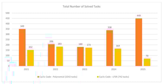
Figure 26.
Total number of solved tasks per year for the wo models solving cyclic code problems.
The Cyclic Code—Polynomial model demonstrates consistently higher activity in all years, reaching a maximum of 449 solved tasks in 2025 and a total of 1542 problems for the entire period. On the other hand, the Cyclic Code—LFSR model shows peak activity in 2022 with 183 solved problems, with the total number for the five-year period being 742 problems.
It is important to note that the LFSR-based model is not mandatory for use in the educational process. It is introduced mainly for demonstration—to present an alternative, machine-based approach to solving problems with cyclic codes. For this reason, its use is entirely at the students’ discretion, which also explains the significantly lower number of solved problems compared to the main Polynomial model, which is mandatory within the exam format.
Figure 27 presents a comparative analysis between the Cyclic Code—Polynomial and Cyclic Code—LFSR models in terms of accuracy in solving problems, distributed according to the number of errors made: 0 errors, 1–2 errors, 3–4 errors, and more than 5 errors.
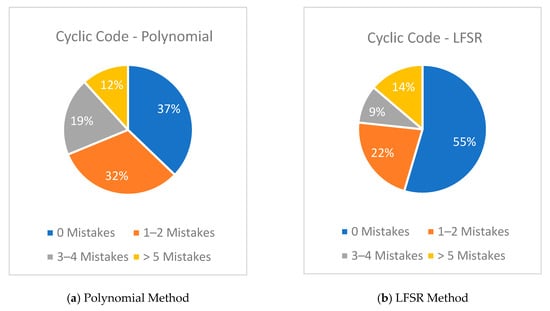
Figure 27.
Distribution of solved tasks by number of errors using the cyclic code models
In the cyclic code—polynomial model, 37% of the problems were solved without errors, and 32% Unfortunately, we could not find the requested information either. The link to the publication does not contain this information. https://mostwiedzy.pl/pl/publication/download/1/user-interface-prototyping-techniques-methods-and-tools_66913.pdfwith, accessed on 28 August 2025. 1–2 errors, which indicates a high level of learning and stable results for the majority of solutions. Only 12% of the solutions contained more than 5 errors, which indicates a relatively good effectiveness of the model as a training tool.
In the cyclic code—LFSR model, the share of problems solved without errors was even higher—55%—which indicates a significantly higher initial success rate. This result can be explained mainly by the fact that the complexity of the algorithm for solving problems using the LFSR model is significantly lower compared to the polynomial model. The simplicity of the method makes it easier for users to apply it, which leads to a lower number of errors when solving. However, the share of tasks with more than 5 errors is 14%, which is slightly higher compared to the polynomial model and is probably due to the rapid and careless execution of repetitive cyclic actions by students, typical of the more mechanical nature of the algorithm.
Figure 28 shows the distribution of the total time spent by each student working with the two interactive models. The data cover the individual total time for solving all tasks by a given student and are extracted through the functionality for automatic registration of tasks in the system. The polynomial model (Cyclic Code—Polynomial) has a higher median of engagement (about 60 min) and a more even distribution, which is in line with its main role in the learning process. On the other hand, the LFSR model has a lower median (about 20 min) and more limited use by some students, as it was designed for informative purposes and is used on a voluntary basis. The presence of outliers in both models indicates variations in the individual pace of work and the depth of engagement. The presented diagrams are not intended for direct comparison, but to illustrate the different patterns of interaction with each of the tools.
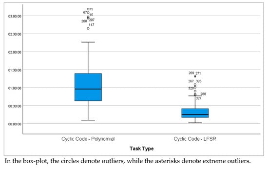
Figure 28.
Distribution of total task-solving time per student for both interactive models.
3.2.3. Student Satisfaction Analysis
Student satisfaction analysis is an essential component in assessing the effectiveness and acceptability of interactive software models used for educational purposes. The survey collects valuable information about students’ personal assessment of the usefulness, accessibility, and impact of the respective tools on the learning process. These data allow us to highlight both the strengths of the developed models and potential areas for improvement. In addition, the level of satisfaction is often related to the intrinsic motivation and active involvement of students, which has a direct impact on the achieved learning results [42].
As part of the study, a survey was conducted to investigate the degree of student satisfaction with various features of the two interactive educational software tools developed to support learning on the topic of cyclic codes. The survey included 74 volunteer participants who rated each of the two models separately using a five-point Likert scale (“Strongly Dissatisfied”, “Dissatisfied”, “Neutral”, “Satisfied”, and “Very Satisfied”). The features evaluated covered key aspects of the user experience, including: “User Interface Design”, “Easy Orientation”, “Website Speed Performance”, “Task-solving Guide”, “Error Statistics”, and “XP Reward Points”.
The survey results for the first training model (polynomial method), given in Figure 29, show a high overall satisfaction among the participants. Most features, including interface design, orientation, and site speed, were rated positively, with the responses “Satisfied” and “Very Satisfied” dominating. The highest satisfaction was reported for the task-solving guide, while the reward points element (XP Reward Points) received more moderate ratings, suggesting potential for improvement in this area.
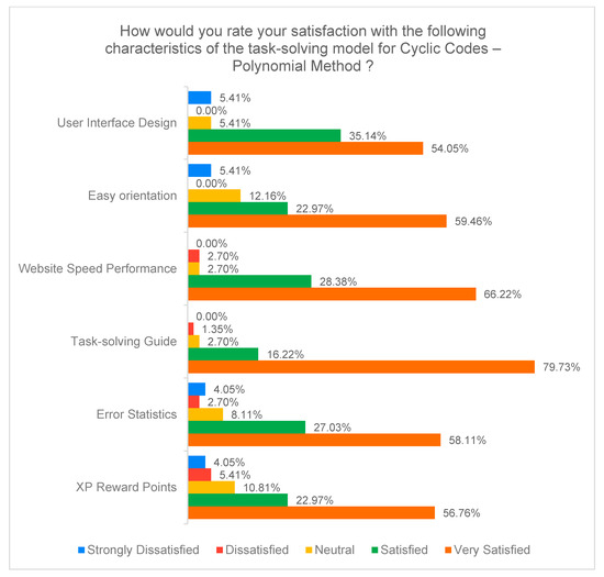
Figure 29.
Results of the survey on the software model for learning Cyclic Code—Polynomial method.
The survey results for the second learning model (LFSR Method) in Figure 30 also show high overall satisfaction among students. Most features, including interface design, orientation, and website speed, were rated primarily as “Satisfied” and “Very Satisfied.” The Problem-Solving Guide again stands out as the highest rated feature, while the “Error Statistics” and “XP Reward Points” features receive more mixed ratings, including some dissatisfaction, indicating room for improvement in these components.
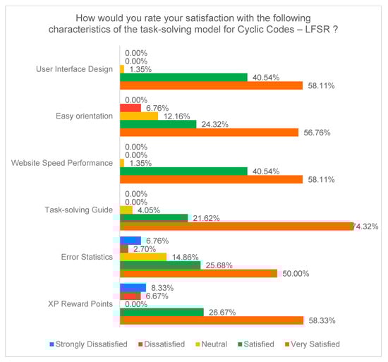
Figure 30.
Results of the survey on the software model for learning cyclic codes—LFSR.
Possible reasons for the lower and more mixed evaluations of the XP Reward Points and Error Statistics functionalities may be related to the way in which students perceive them. In the case of XP Reward Points, it is possible that some students do not see a direct connection with the acquisition of the learning content and perceive it as a game element, while others would expect a more flexible and motivating incentive system. Regarding Error Statistics, it is possible that for some students this feature is useful for self-reflection, but for others it is perceived as an unnecessary burden or an additional assessment element. These hypothetical reasons may explain the diversity in the feedback and indicate that there is potential for improvements aimed at emphasizing the pedagogical value and practical applicability of both functionalities.
4. Discussion
The present study is part of a broader line of developments aimed at the application of interactive software tools in coding training in information and communication systems. The applied methodology, already validated in previous studies, was adapted to the specifics of cyclic codes and the corresponding algorithms. This allowed not only the design and testing of a functional training tool, but also the collection of significant empirical data on its pedagogical effectiveness.
The most significant result of the study is related to the pedagogical experiment, in which the results of the control and experimental group of students are compared. The analysis found a statistically significant difference in the average grade in the initial state in favor of the experimental group. To compensate for this effect, an ANCOVA analysis was applied, which takes into account the influence of the initial success on the final results. After the correction, the advantage of the experimental group was preserved, which shows that the use of interactive models has a positive contribution to increasing success rates, regardless of the initial level of students.
The statistics of solved tasks and student engagement show clear differences between the two training models. The polynomial model was used by a larger number of users and, accordingly, maintained longer-term engagement. This is probably due to both the nature of the tasks, requiring precise arithmetic operations with polynomials, and the fact that this model is subject to self-assessment and plays a major role in forming the final grade. In turn, the LFSR model, although used more limitedly, is distinguished by high accuracy in solving tasks. Its main purpose is illustrative—it supports the intuitive understanding of the process of forming a code word by visualizing the dynamics of register operations. Although work with it is not assessed independently, the degree of engagement is also taken into account when forming the final grade.
In a pedagogical context, the two models perform complementary functions. The polynomial model supports the development of analytical skills and mathematical precision, while the LFSR approach promotes conceptual understanding through visual interaction. This combination is consistent with the principles of multimodal learning, according to which a variety of presentation formats facilitate the learning of complex technical concepts.
Feedback from students—both through a survey and observation during actual use—played a significant role in improving the interface and functionality of the models. Although not all components were rated equally highly, the overall satisfaction supports the thesis that well-designed software tools can be an effective means of supporting learning in technical disciplines.
The results of this study are largely consistent with global trends in digital education, according to which the use of interactive and multimodal tools leads to higher engagement and better learning outcomes. Similar studies in engineering and computer science education show that software models support deeper conceptual understanding and lasting knowledge acquisition compared to traditional approaches, which confirms the effectiveness of the applied methodology.
5. Conclusions
This article presents the process of designing, developing, and evaluating two interactive software training models focused on the topic of “cyclic codes”—the first one based on the polynomial method, and the second one on the LFSR approach. The development is based on an established methodology, successfully applied in previous studies, and in the present work, it was adapted to the specifics of the content and technical requirements of the two models.
The conducted experimental study covered three main aspects: educational effectiveness, student engagement, and satisfaction. The most significant result stems from the pedagogical experiment, which demonstrates a statistically significant advantage of the experimental group even after correction through ANCOVA analysis. This confirms the positive effect of using interactive models on student achievement.
The two models perform complementary pedagogical roles: The polynomial model encourages analytical thinking and precision through arithmetic operations, while the LFSR model visualizes key processes and supports intuitive understanding of algorithms. For example, the learning process can begin with the polynomial model, which provides an opportunity to follow the step-by-step algorithmic training and gain a deeper understanding of the mathematical basis. Students can then move on to the LFSR model, which visualizes the operation of the CRC in register form, thus reinforcing conceptual understanding through clarity and a practical perspective. This combination corresponds to the principles of multimodal learning and allows for a more flexible and targeted approach to the mastery of complex technical topics.
Based on the collected quantitative data and feedback from students, the strengths of the applied models were identified as well as specific opportunities for improvement. Some of the suggestions have already been implemented through interface updates, functionality optimization, and the addition of new support elements. The accumulated experience and results create a good basis for expanding the approach to other topics in technical disciplines and for further validation of the methodology used.
In the future, there are several directions for further development of the system in accordance with modern trends in digital education. One of them is the integration of artificial intelligence (AI) in order to automatically generate conditions for tasks with adaptive difficulty, tailored to the individual progress of each student. Another potential direction is the use of AI to analyze data from student activity and provide an objective assessment of progress, which would facilitate the teacher in forming the final grades.
In parallel, a new gamified mode of working with the learning models is under development, in which tasks are presented in a sequence of increasing difficulty, and students receive different virtual badges depending on the results achieved. The aim of this approach is to strengthen the motivation and long-term engagement of learners by creating a more interactive and satisfying educational environment.
The present study successfully achieves the goal set at the beginning—the creation of two interactive models for studying cyclic codes and their experimental investigation. The results show that the use of the models increases learning outcomes, increases student motivation, and supports the conceptual understanding of algorithmic processes. In this way, the pedagogical value and practical applicability of the proposed models in a virtual laboratory in coding theory are demonstrated.
6. Limitations of the Study
Several limitations should be noted. First, the control and experimental groups were formed in different time periods, which may affect their full comparability. It should be noted that the control group was studied before the COVID-19 pandemic, while the experimental group was studied after the pandemic. During this period, digital and hybrid practices became widespread, significantly affecting students’ digital literacy. Due to the post facto nature of the control group study, it was not possible to directly measure the digital abilities of students from the different groups, which means that this factor cannot be accounted for in the present study. This contextual difference should be considered when interpreting the results.
Second, the initial level indicator used—the grade point average from the previous two semesters—does not directly measure knowledge on the subject, although it provides a reliable basis for comparison. Third, the study was conducted within a single university and with a limited sample, which limits the possibility of generalizing the results. Despite these limitations, the data obtained outline clear trends and prerequisites for future research.
Author Contributions
Y.A. proposed the conceptual idea. Y.A. analyzed the existing solutions and studied the possibilities and necessities of creating such a system. Y.A. and A.B. contributed to the literature review. G.I. utilized the interactive model in the learning process, conducted practical exercises and control works with students using the system, and collected information on the grades. Y.A. and A.B. designed the plan and structure of the pedagogical experiment. Y.A. made a statistical comparison of the average grades between the control and experimental groups as well as a statistical analysis of the students’ activity and the usability of the interactive model. G.I. formulated the questions and conducted and analyzed the results of the student satisfaction survey. The writing (original draft preparation) was undertaken by Y.A., and the review and editing processes were anyzed by A.B. All authors have read and agreed to the published version of the manuscript.
Funding
This study is financed by the European Union–NextGenerationEU, through the National Recovery and Resilience Plan of the Republic of Bulgaria, project № BG-RRP-2.013-0001.
Institutional Review Board Statement
Not applicable.
Informed Consent Statement
Not applicable.
Data Availability Statement
All data used in the statistical study of this research can be accessed at the following address: https://ecsunirusebg-my.sharepoint.com/:f:/g/personal/yaliev_ecs_uni-ruse_bg/Elxuh-njRM1Pv4Mg2EyiYP0B3LuvX50p2LRWjpKPiG63TQ?e=y3paKa (accessed on 31 July 2025).
Conflicts of Interest
The authors declare no conflicts of interest.
References
- European Commission, Digital Education Action Plan (2021–2027). Available online: https://education.ec.europa.eu/focus-topics/digital-education/plan (accessed on 23 August 2025).
- OECD. OECD Digital Education Outlook 2023. Available online: https://www.oecd.org/education/2023/digital-education-outlook-2023.html (accessed on 23 August 2025).
- Domínguez, A.; Saenz-de-Navarrete, J.; De-Marcos, L.; Fernández-Sanz, L.; Pagés, C.; Martínez-Herráiz, J.J. Gamifying learning experiences: Practical implications and outcomes. Comput. Educ. 2013, 63, 380–392. [Google Scholar] [CrossRef]
- Nah, F.F.H.; Zeng, Q.; Telaprolu, V.R.; Ayyappa, A.P.; Eschenbrenner, B. Gamification of education: A review of literature. In International Conference on Hci in Business; Springer International Publishing: Cham, Switzerland, 2014; pp. 401–409. [Google Scholar]
- Mayer, R.E. (Ed.) The Cambridge Handbook of Multimedia Learning; Cambridge University Press: Cambridge, UK, 2005. [Google Scholar]
- Podolefsky, N.S.; Moore, E.B.; Perkins, K.K. Implicit scaffolding in interactive simulations: Design strategies to support multiple educational goals. arXiv 2013, arXiv:1306.6544. [Google Scholar]
- Shute, V.J. Focus on formative feedback. Rev. Educ. Res. 2008, 78, 153–189. [Google Scholar] [CrossRef]
- Chiotaki, D.; Poulopoulos, V.; Karpouzis, K. Adaptive game-based learning in education: A systematic review. Front. Comput. Sci. 2023, 5, 1062350. [Google Scholar] [CrossRef]
- Ministry of Education, Government of India. Virtual Labs Initiative Official Website. Available online: https://www.vlab.co.in (accessed on 18 July 2025).
- Virtual Labs Initiative. Cyclic Code Simulation System. Available online: https://virtual-labs.github.io/exp-cyclic-codes-iiith/index.html (accessed on 18 July 2025).
- Diwakar, A.S.; Noronha, S.B. The effectiveness of virtual labs in engineering education-what do we measure? J. Eng. Educ. Transform. 2016, 30, 73–81. [Google Scholar] [CrossRef]
- Li, J.; Liang, W. Effectiveness of virtual laboratory in engineering education: A meta-analysis. PLoS ONE 2024, 19, e0316269. [Google Scholar] [CrossRef] [PubMed]
- Aliev, Y.; Ivanova, G.; Borodzhieva, A. Design and Development of Interactive Software Models for Teaching Coding Theory: A Case Study on Hamming Codes—General Algorithm. Appl. Sci. 2025, 15, 4231. [Google Scholar] [CrossRef]
- Aliev, Y.; Ivanova, G.; Borodzhieva, A. Design and Research of a Virtual Laboratory for Coding Theory. Appl. Sci. 2024, 14, 9546. [Google Scholar] [CrossRef]
- Lampropoulos, G.; Kinshuk, H. Virtual reality and gamification in education: A systematic review. Educ. Tech. Res. Dev. 2024, 72, 1691–1785. [Google Scholar] [CrossRef]
- Camacho-Sánchez, R.; Rillo-Albert, A.; Lavega-Burgués, P. Gamified digital game-based learning as a pedagogical strategy: Student academic performance and motivation. Appl. Sci. 2022, 12, 11214. [Google Scholar] [CrossRef]
- Kebande, V.R. The impact of virtual laboratories on active learning and engagement in cybersecurity distance education. arXiv 2024, arXiv:2404.04952. [Google Scholar] [CrossRef]
- Dustman, W.A.; King-Keller, S.; Marquez, R.J. Development of gamified, interactive, low-cost, flexible virtual microbiology labs that promote higher-order thinking during pandemic instruction. J. Microbiol. Biol. Educ. 2021, 22, 10–1128. [Google Scholar] [CrossRef]
- Rosli, R.; Ishak, N.A. Integration of Virtual Labs in Science Education: A Systematic Literature Review. J. Pendidik. Sains Dan Mat. Malays. 2024, 14, 81–103. [Google Scholar] [CrossRef]
- Rahman, F.; Mim, M.S.; Baishakhi, F.B.; Hasan, M.; Morol, M.K. A Systematic Review on Interactive Virtual Reality Laboratory. arXiv 2022, arXiv:2203.15783. [Google Scholar] [CrossRef]
- Gagnon, D.J. ARIS: An Open Source Platform for Developing Mobile Learning Experiences. arXiv 2023, arXiv:2302.09291. [Google Scholar] [CrossRef]
- Alabiad, S.; Alkhamees, Y. A Unique Representation of Cyclic Codes over GR(pn,r). Axioms 2022, 11, 519. [Google Scholar] [CrossRef]
- An, W.; Médard, M.; Duffy, K.R. CRC codes as error correction codes. In Proceedings of the ICC 2021-IEEE International Conference on Communications, Montreal, QC, Canada, 14–23 June 2021; pp. 1–6. [Google Scholar]
- Gautam, A.; Thakur, P.; Singh, G. Analysis of Universal Decoding Techniques for 6G Ultra-Reliable and Low-Latency Communication Scenario. Future Internet 2025, 17, 181. [Google Scholar] [CrossRef]
- Clark, R.C.; Mayer, R.E. E-Learning and the Science of Instruction: Proven Guidelines for Consumers and Designers of Multimedia Learning; John Wiley & Sons: Hoboken, NJ, USA, 2023. [Google Scholar]
- Sklar, B. Digital Communications: Fundamentals and Applications; Prentice Hall: Upper Saddle River, NJ, USA, 2001. [Google Scholar]
- Chawla, G.; Chaudhary, V. FPGA Implementation of Cyclic Code Encoder and Decoder, Advance in Electronic and Electric Engineering. Adv. Electron. Electr. Eng. 2014, 4, 273–278. [Google Scholar]
- Weichbroth, P.; Sikorski, M. User interface prototyping. Techniques, methods and tools. Stud. Ekonomiczne. Zesz. Nauk. Uniw. Ekon. W Katowicach 2015, 184–198. [Google Scholar]
- Balsamiq. Balsamiq Wireframes. 2008. Available online: https://balsamiq.com (accessed on 18 July 2025).
- Mackie, S.; Mason, R.; Hibbard, J.; Walker, A. JavaScript: Best Practice; SitePoint Pty. Ltd.: Melbourne, Australia, 2018. [Google Scholar]
- WHATWG. HTML Standard. Available online: https://html.spec.whatwg.org/multipage/ (accessed on 18 July 2025).
- Tittel, E.; Noble, J. HTML, XHTML and CSS for Dummies; John Wiley & Sons: Hoboken, NJ, USA, 2011. [Google Scholar]
- The jQuery Foundation. (n.d.). jQuery—JavaScript Library. Available online: https://jquery.com (accessed on 18 July 2025).
- Konva.js. (n.d.). Konva.js—HTML5 2D Canvas JS Library for Desktop and Mobile Applications. Available online: https://konvajs.org (accessed on 18 July 2025).
- Tatroe, K.; MacIntyre, P. Programming PHP: Creating Dynamic Web Pages; O’Reilly Media, Inc.: Sebastopol, CA, USA, 2020. [Google Scholar]
- DuBois, P. MySQL; Addison-Wesley: Boston, MA, USA, 2013. [Google Scholar]
- Bruegge, B.; Dutoit, A.H. Object Oriented Software Engineering: Using UML Patterns and Java; Prentice Hall: Upper Saddle River, NJ, USA, 2010. [Google Scholar]
- Field, A. Discovering Statistics Using IBM SPSS Statistics; SAGE Publications Ltd.: Thousand Oaks, CA, USA, 2013. [Google Scholar]
- Mohammed, A.; Shayib, A. Applied Statistics, 1st ed.; Bookboon: London, UK, 2013; ISBN 978-87-403-0493-0. [Google Scholar]
- Stevens, J.P. Applied Multivariate Statistics for the Social Sciences, 5th ed.; Routledge: New York, NY, USA, 2012. [Google Scholar]
- Rutherford, A. ANOVA and ANCOVA: A GLM Approach; John Wiley & Sons: Hoboken, NJ, USA, 2011. [Google Scholar]
- Liu, Y.; Ma, S.; Chen, Y. The impacts of learning motivation, emotional engagement and psychological capital on academic performance in a blended learning university course. Front. Psychol. 2024, 15, 1357936. [Google Scholar] [CrossRef] [PubMed] [PubMed Central]
Disclaimer/Publisher’s Note: The statements, opinions and data contained in all publications are solely those of the individual author(s) and contributor(s) and not of MDPI and/or the editor(s). MDPI and/or the editor(s) disclaim responsibility for any injury to people or property resulting from any ideas, methods, instructions or products referred to in the content. |
© 2025 by the authors. Licensee MDPI, Basel, Switzerland. This article is an open access article distributed under the terms and conditions of the Creative Commons Attribution (CC BY) license (https://creativecommons.org/licenses/by/4.0/).