Article

Predictive Modeling for Carbon Footprint Optimization of Prestressed Road Flyovers

by
Lorena Yepes-Bellver
1,†,
Julián Alcalá
2 and
Víctor Yepes
2,*,†
1
Mechanics of Continuous Media and Theory of Structures Department, Universitat Politècnica de València, 46022 Valencia, Spain
2
Institute of Concrete Science and Technology (ICITECH), Universitat Politècnica de València, 46022 Valencia, Spain
*
Author to whom correspondence should be addressed.
These authors contributed equally to this work.
Appl. Sci. 2025, 15(17), 9591; https://doi.org/10.3390/app15179591
Submission received: 27 July 2025 / Revised: 15 August 2025 / Accepted: 28 August 2025 / Published: 31 August 2025
(This article belongs to the Section Ecology Science and Engineering)

Abstract

This study addresses the challenge of minimizing carbon emissions in designing prestressed road flyovers by comparing advanced predictive modeling techniques for surrogate-based optimization. The research develops a two-stage optimization approach. First, a response surface is generated using Latin-hypercube sampling. Second, that response surface is optimized to identify design configurations with the lowest CO2 emissions. The optimal configuration (deck #37)—base width 3.40 m, deck depth 1.10 m, and concrete grade C-35 MPa—achieved a carbon footprint of 386,515 kg CO2, representing a reduction of 12% compared to the reference bridge. Among the models tested, the artificial neural network (ANN) achieved the highest predictive accuracy (RMSE = 8372 kg, MAE = 7356 kg), closely followed by the Kriging 1 model (RMSE = 9235 kg, MAE = 7236 kg). Results indicate that emissions remain minimal for deck depths between 1.10 and 1.30 m, base widths between 3.20 and 3.80 m, and concrete grades of C-35 to C-40 MPa. This study provides practical guidelines for reducing the carbon footprint of prestressed bridges and highlights the value of robust surrogate models in sustainable structural optimization.

1. Introduction

Minimizing carbon emissions remains a challenge in combating climate change, as it affects all aspects of human activity [1]. The construction sector holds a significant role, consuming 15% of the world’s freshwater and accounting for 50% of global material extraction, while also contributing 37% of CO2 emissions related to energy use [2]. Among these, concrete production for construction accounts for over 5% of the total carbon footprint [3]; thus, emission reductions represent an essential pillar of research needed to create a more sustainable industry [4,5,6].
The sustainable construction of bridges is essential to support infrastructure development while maintaining long-term environmental, social, and economic balance. While bridges offer significant benefits, they also present significant challenges in these areas due to the CO2 emissions generated throughout their life cycle. Embodied carbon focuses explicitly on the greenhouse gases generated during the production of a product, including extraction, transport, and manufacturing processes. A comprehensive review has been undertaken to summarize the values associated with embodied carbon and energy [7].
Recent work [8] has underlined how inventory models and carbon-pricing mechanisms interact with technology investment and operational decisions; these mechanisms can materially change the optimal engineering choices at the project level (e.g., green inventory under carbon tax, cap-and-trade, and offset regimes).
Since ancient times, designs have been improved. The right choice of materials or their optimal design can reduce emissions. Bridges are vital, and the performance of prestressed concrete (PC) bridges depends on the engineer’s experience. Although the design follows standard practices, its approval is obtained through trial and error, leading to variable costs despite code compliance. Structural optimization methods provide other avenues for design solutions that are not based solely on experience.
Structural optimization is typically carried out using two primary approaches [9]. The first involves exact methods, usually based on mathematical programming techniques. The second strategy relies on artificial intelligence-driven heuristic algorithms frequently inspired by nature. These algorithms have shown outstanding ability and adaptability in complex, large-scale optimization problems with non-linear characteristics typical in structural optimization problems [10]. Due to the nature of structural optimization problems, heuristic methods are frequently applied to solve them.
Additionally, studies from the supply chain and operations research communities demonstrate that integrated inventory and operational strategies can balance cost, product deterioration, and carbon emissions, and that multi-echelon supply chain design influences the environmental outcomes of infrastructure supply chains—insights that are conceptually relevant when inspecting material selection and logistics for bridge construction [11,12].
The significant disadvantage of structural design heuristics is the high cost of computation [13]. Approximations or surrogate models, generally known as metamodels, are used to solve this problem. A metamodel can be a replacement for a simulation model that can cut down the computational effort significantly. Some of the most common surrogate models used for structural design optimization are Kriging or Artificial Neural Networks (ANNs). Although applied to real-world structural design only to a limited extent, Kriging is nonetheless one of the most promising approaches. For example, Kriging has been used to settle articulated structure design, efficiently decoupling uncertainty quantification from optimizing [14]. This method has also been extended successfully to other domains, such as the design of prestressed bridges [15,16], the optimization of structural systems [17], the development of architectural models for residential structures [18], and the prediction of carbonation depths in concretes [19]. ANNs learn from training data and produce outputs by evaluating the non-linear relations among their inputs. Researchers utilize them to forecast structural performance [20] and aid in the multiobjective optimization of structures [21]. Radial basis functions (RBFs) have been employed for structural health monitoring of composite laminated beams [22] and frequency-domain structural damage identification in multi-member structures [23]. Gaussian process regression (GPR) has been applied to perform system fragility analysis of highway bridges using multi-output surrogate models [24] and to detect structural damage in bridges under varying temperature effects through hybrid data training approaches [25]. These examples illustrate the breadth of practical engineering problems where such surrogate models have been successfully integrated, reinforcing their relevance for the present research.
Overpasses are commonly constructed using continuous PC beams, suitable for spans between 10 m and 45 m. Slab solutions are competitive with precast beams due to their structural and construction advantages, such as adapting to complex layouts, simpler formwork, and eliminating pavement joints. Slab bridges are cost-effective for complex geometric conditions, like curves or low road heights. Traditional formwork systems are typically employed for spans beginning at 20 m and up to four spans (under 120–140 m). For longer spans, self-supporting formwork is required. Slab sections are concreted in situ for 30 m to 60 m spans, with cantilevering used for spans over 25 m.
Despite advancements, further research is needed to optimize embodied carbon in bridges. A hybrid firefly based heuristic was used to optimize a prefabricated trough girder bridge, displaying that a €1 cost reduction resulted in 1.75 kg of CO2 [26]. Another investigation focused on optimizing a post-tensioned box-section pedestrian bridge, revealing that emissions can be minimized by increasing edge dimensions, adding more active cables, and reducing the concrete grade [27]. Multiobjective optimization was also conducted for a PC box girder bridge [28] and T-girder bridges [29]. A life-cycle assessment of a precast bridge revealed that the manufacturing use and maintenance phases have a higher environmental impact [30].
Studies comparing different metamodels have not determined a clear superior type [31,32]. Ryberg [33] highlights that performance is affected by parameter tuning, which varies depending on the software used. Radial basis functions (RBF) proved effective for scenarios with limited sample sizes, primarily due to their ease of implementation [34]. Kriging offers better accuracy with larger sample sizes when adequately calibrated. RBF is generally more reliable, though these studies have limitations, such as fixed parameters and few variables. Elwy and Hagishima [35] provide an up-to-date overview of optimization techniques supported by metamodels in building design.
This study analyzes the response surface generated by various metamodels to compare the predicted values from each model. It also examines how these models can identify the most advantageous features for predesigning PC slab bridges to moderate the CO2 footprint in their construction process.

2. Materials and Methods

2.1. Case Study: Description of the Lightweight Prestressed Slab Bridge

The study aims to optimize the carbon footprint design of a deck for a post-tensioned road flyover prestressed and lightened slab with 24–34–28 m spans, typical of dual carriageway overpasses. As shown in Figure 1 and Figure 2, the slab has a rectilinear geometry with uniform depth and a deck width of 8.30 m, designed to carry two traffic lanes, each measuring 3.50 m. It features parapets of 0.65 m on both sides. Figure 1 and Figure 2 illustrate the geometry of the studied deck: Figure 1 shows the longitudinal view of the lightweight prestressed slab. In contrast, Figure 2 shows the cross-section, main dimensions, and hollow-core configuration used in the analysis.
This overpass, located at the 441st kilometer of the A-7 motorway near Cocentaina in the Alicante region, features the width of the base b = 4.00 m, a depth c = 1.35 m, and a cantilever length v = 1.75 m. Its sizes include c1 = 0.30 m, c2 = 0.20 m, and d = 0.40 m. The internal voids consist of four cylinders with a diameter ϕ = 0.60 m each, with internal voids measuring 0.14 m3/m2 and the external voids of 0.51 m3/m2.
The limit state design ensures structural safety by applying partial safety factors. Each design scenario is evaluated to confirm that the slab bridge does not exceed any limit states. The deck was modeled, analyzed, and designed using the CSiBridge@ Version 21.0.0 software. Evaluating each slab bridge’s structural response provided the acting stresses, represented as sectional forces. Additionally, the stress resultants for each element were calculated, reflecting the resistance sectional stresses. Stresses are determined independently based on the configuration of each structural component. Further information regarding the structural calculations can be found in [15,16].

2.2. Inputs and Carbon Inventory

The building of each deck generates CO2 emissions, which are influenced by the concrete grade, the formwork, the amount of lighting, and the amount of steel. The emissions have been assessed, as shown in Table 1 [36].
The construction uses Y-1860-S7 and B-500-S steel. The concrete grade ranges from 30 to 50 MPa. Additionally, using lightweight materials helps the overall weight, enhancing performance and cost-effectiveness. The slab formwork is critical in supporting and shaping the concrete, influencing the surface quality and the construction speed.

2.3. Sampling and Optimization Strategy

A previous study [15] proposed a two-phase methodology for optimizing the response surface, modeled using Kriging. This approach predicts embodied carbon using the MATLAB Kriging Toolbox, Version 2.0 (DACE) to construct the metamodel [37]. A set of 30 bridges was selected through Latin hypercube sampling (LHS), which generates random numbers with a uniform distribution to evaluate alternatives. LHS provides lower sample mean-variance compared to random sampling [38]. The approach involves selecting a random sample from each variable interval, ensuring that the entire range of each variable is explored while maintaining a structured, low-discrepancy sampling pattern. LHS improves the understanding of the design space, reduces systematic errors, ensures uniform sampling across the space, and is particularly suitable for computational testing. It offers flexibility, efficiency, and rapid result generation. A list of all the decks considered is provided in Table 2.
The Kriging response surface was optimized with the first 30 data points in the diversification phase, while the intensification phase employs the subsequent five data points. In the first phase of diversification, the response surface was optimized using simulated annealing. Following this, a further sampling of five additional decks was conducted around the previously identified optimum, and the surface was re-optimized. This process led to discovering a new optimum in the intensification phase.

2.4. Surrogate Models

This research seeks to assess the performance of different predictive models to determine how much they can capture the information from the actual response surface. These techniques are chosen based on their proven ability to handle optimization problems with complex, non-linear response surfaces, such as those presented in this case. Various metrics will be defined to assess the error between the actual unknown data and the model’s predictions.

2.4.1. Radial Basis Functions

Radial basis functions (RBFs) [39] are among the methods used to construct complex systems’ surrogate models through function fitting and data-driven modeling. These functions are based on the principle of radial symmetry, which implies that their output depends solely on the distance between a target point and a central reference. RBFs exhibit strong performance when reconstructing values from irregularly distributed datasets, enabling the generation of continuous and differentiable approximations that remain robust in complex, multi-dimensional domains. An RBF, with input variables xi collectively represented as xi, can be defined as:
f x = i = 1 N Φ Φ i x α i + b x
In this context, f = f(x) represents the output response, Φi = Φi(x) are the RBFs, NΦ indicates the number of RBFs, αi are the associated weights, and b = b(x) denotes the bias term. The number of RBFs selected corresponds to the number of input variables.
The particular type of RBF chosen—such as linear, Gaussian, or thin plate spline— has an impact on the model’s flexibility and smoothness. The selected RBF variants (linear, multiquadratic, inverse multiquadratic, and cubic) were chosen because they collectively span a range of smoothness and flexibility properties while remaining numerically stable for small-sample problems. Prior comparative studies in engineering metamodeling have shown that these kernels provide a practical trade-off between flexibility and overfitting in problems with moderate dimensionality and limited observations [34,39]. Thus, evaluating this set enables a representative comparison of the radial basis functions used in structural-design surrogate modeling. The most commonly applied types of RBFs include the following:
L i n e a r :   Φ i r = r
M u l t i q u a d r a t i c :   Φ i r = r ε i 2 + 1
I n v e r s e   m u l t i q u a d r a t i c :   Φ i r = 1 r ε i 2 + 1
C u b i c :   Φ i r = r 3
where r represents the Euclidean distance and ( ε i ) denotes the shape parameter.

2.4.2. Kriging Metamodel

Kriging [40] predicts the value of a specific location u using a collection of n observed z-values (Figure 3). In this case, the focus is on estimating the embodied carbon of the bridge deck. This technique allows for response predictions without requiring comprehensive structural analysis. Kriging models produce consistent results as deterministic functions when applied to the same known data without random errors. The general expression for a Kriging model is given by:
y x = f x + Z ( x )
In this formulation, Z(x) represents a stochastic residual with zero mean and spatial dependence, typically characterized through a correlation structure. Meanwhile, f(x) is the approximation function, similar to a regression model. This function captures the non-random tendency in the data—the part governed by known or predictable relationships—and is commonly expressed as follows:
f x = i = 1 n β i f i ( x )
In this context, fi(x) denotes the predefined basis functions—such as low-order polynomials or other simple functional forms—while βi are parameters to be estimated, which characterize the mean or trend component. This component can be represented in various forms: as an invariant mean in Ordinary Kriging, zero in Simple Kriging, or as a polynomial (e.g., linear or quadratic) in Universal Kriging. This study uses polynomial regressions of orders zero, one, and two to construct models labeled Kriging 1, Kriging 2, and Kriging 3, respectively. These models produce specified predictions, generating the same output for identical inputs when no random error exists.
In this study, the Kriging models were implemented using the MATLAB DACE toolbox [37], which estimates correlation parameters (including separate length scales for each input dimension and the nugget term) via maximum likelihood estimation. The nugget parameter, representing observation noise, was included with a small value to improve numerical stability, given the deterministic nature of the dataset. Anisotropy was addressed by independently estimating length scales for each design variable, allowing different correlation ranges per dimension. The Gaussian radial basis function (RBF) kernel was selected due to its proven robustness in structural optimization problems with small datasets [34,39]. Preliminary tests with alternative kernels, such as the Matérn and exponential functions, did not improve the cross-validated RMSE for the present dataset.

2.4.3. Artificial Neural Networks

An artificial neural network (ANN) comprises a structure that begins with an input node layer, followed by one or more intermediate hidden layers, and output layers, enabling the detection of intricate links among variables. The input layer receives the data, which is then processed by the hidden layer. The model undergoes training by iteratively adjusting the weights and backpropagating errors to enhance its accuracy. A detailed overview of ANN’s fundamental concepts, recent developments, and practical uses can be found in [41]. At the same time, additional discussions focus on their practical use and effectiveness, highlighting their broad applicability and proven impact [42].
A multilayer feedforward network is organized with an intermediate layer containing sigmoidal neurons, while the final layer consists of linear neurons. The hidden layer neurons are interconnected with the initial and final layers, with the hidden layer neuron number proportional to the initial and final parameter numbers.
The entry variables (xi) are scaled by their associated weights (wi,j) and subsequently offset by the addition of a bias term (bj). Every node in the hidden layer calculates the following equation: ∑xiwi,j + bj. The output of each hidden unit is then generated by applying a sigmoid tangent function to this equation. In contrast, the final layer uses a linear function. This architecture, known as the multilayer perceptron (MLP), is widely utilized for approximating various functions, even when only a single hidden layer is utilized [43]. The backpropagation algorithm contributes to its success in modeling complex relationships by optimizing the weights and biases through error correction in training [44,45].
In a feed-forward network, data moves from the initial to the final layer, with learning tracked using data with predefined responses. The dataset is split into three subsets to assess overfitting: a training dataset for adjusting parameters, a validation dataset to detect overfitting, and a test set to assess the forecasting performance of the model on previously unseen data. The “early stopping” technique mitigates overfitting without explicitly partitioning the dataset into separate training and validation subsets. During the optimization process, performance metrics are monitored on both components to guide termination. If training errors continue to decrease while validation errors rise, this signals potential overfitting, prompting the termination of further training. In that case, the optimization progression is halted, preventing overlearning and ensuring the model can generalize effectively.
The neural network randomly chose 30 data points (24 training, 3 validation, and 3 test). The network architecture features a single hidden layer comprising five neurons. Simulation assesses model performance by generating predictions based on either training or previously unseen data, followed by an outcomes analysis. The initial stage involves cross-validation, a process that compares the output from the training phase with the results produced by the neural network simulation. This step is essential to assess the model’s accuracy and identify overfitting, which occurs when the model becomes excessively fitted to the training data. Cross-validation can be conducted across various partitions of the dataset—namely, training, validation, and test sets—to examine the risk of overfitting comprehensively.
The ANN models were implemented using MATLAB’s Neural Network Toolbox [46], employing the mean squared error (MSE) as the loss (performance) function during training. Network performance was monitored via MATLAB’s built-in performance plots, which display the MSE on the training, validation, and test sets across iterations, enabling visual detection of overfitting. Overfitting was controlled using the early stopping technique, where training was halted if the validation error did not improve for a predefined number of iterations. The architecture comprised a single hidden layer with five neurons, selected after preliminary trials to balance predictive accuracy and network simplicity for the small dataset. The 30 available samples were divided into 24 for training, 3 for validation, and 3 for testing. Given the limited dataset size, multiple independent runs with different random partitions were performed, and the predictions were averaged to improve robustness and reduce the influence of any single partition.

2.4.4. Gaussian Process Regression

The Gaussian Process Regression (GPR) model is a flexible, data-driven approach that does not rely on a fixed set of parameters offering a probabilistic regression framework [47]. It is advantageous when the relationship between entries and exits is complex and non-linear, as it can capture various underlying patterns. The Matern 5/2 kernel was used in this study [48], as it is well-suited for modeling smooth, non-linear relationships. Automatic hyperparameter optimization was employed to adjust the kernel parameters, enhancing the model and minimizing prediction errors. Both input and output variables were normalized using Z-score normalization to standardize the scale, which is crucial because GPR models are sensitive to data scaling.
Cross-validation with exclusion was employed to assess the model’s effectiveness and generalizability. The data were partitioned, with 80% assigned to training and 20% to testing. The model was developed using the training set, while the test dataset was used to evaluate its predictive accuracy. This technique reduces overfitting and ensures the model can predict new data.
To address the stochastic nature of the GPR model, 16 independent runs were conducted with different random seeds. The predictions were then averaged to minimize variability and yield more consistent results. This repetition, with distinct random seeds for each run, accounts for the model’s inherent variability due to random initialization, ensuring that the predictions are not overly influenced by the initial conditions of the optimization process and offering a more robust model performance evaluation.
The predictions obtained in the normalized domain were reverted to their original scale by applying the appropriate inverse transformation. The final output comprised the averaged predictions for the new data points denormalized to the original scale. Cross-validation and hyperparameter optimization were used to guarantee the reliability and robustness of the predictions.
A robust and dependable model was developed through the integration of Gaussian Process Regression with hyperparameter optimization, data normalization, and the averaging of predictions. By averaging across multiple runs, the model’s prediction stability was enhanced, effectively capturing the inherent stochasticity of the process and yielding consistent and reliable results.

2.5. Model Evaluation Metrics

Various metrics are employed to analyze the discrepancies between the actual results of novel solutions and their respective predicted values to evaluate the accuracy of the different models. Each model undergoes an evaluation process, assessing performance metrics to determine reliability and effectiveness [49]. Metrics include root mean square error (RMSE), mean absolute error (MAE), and the ratio of RMSE to the standard deviation of observations (RSR). These measurements give information on the model’s predictive ability under different conditions. Comparing estimations against error thresholds ensures robust performance assessment. The formulae for these metrics are given at (8)–(10).
R M S E = i = 1 n y ^ i y i 2 n
R S R = R M S E S D
M A E = i = 1 n y ^ i y i n
where y ^ i are the expected values, yi denote the real values, and n corresponds to the total count of observations. SD refers to the observation’s standard deviation.

3. Results

In the initial diversification phase, the response surface was optimized using the simulated annealing algorithm, yielding deck #36 as the optimal solution. Subsequently, five additional decks were sampled near this optimum, and the surface was re-optimized. This second optimization, carried out during the intensification phase, identified a new optimum corresponding to deck #37. The local optima for each phase are represented by #36 and #37, respectively.
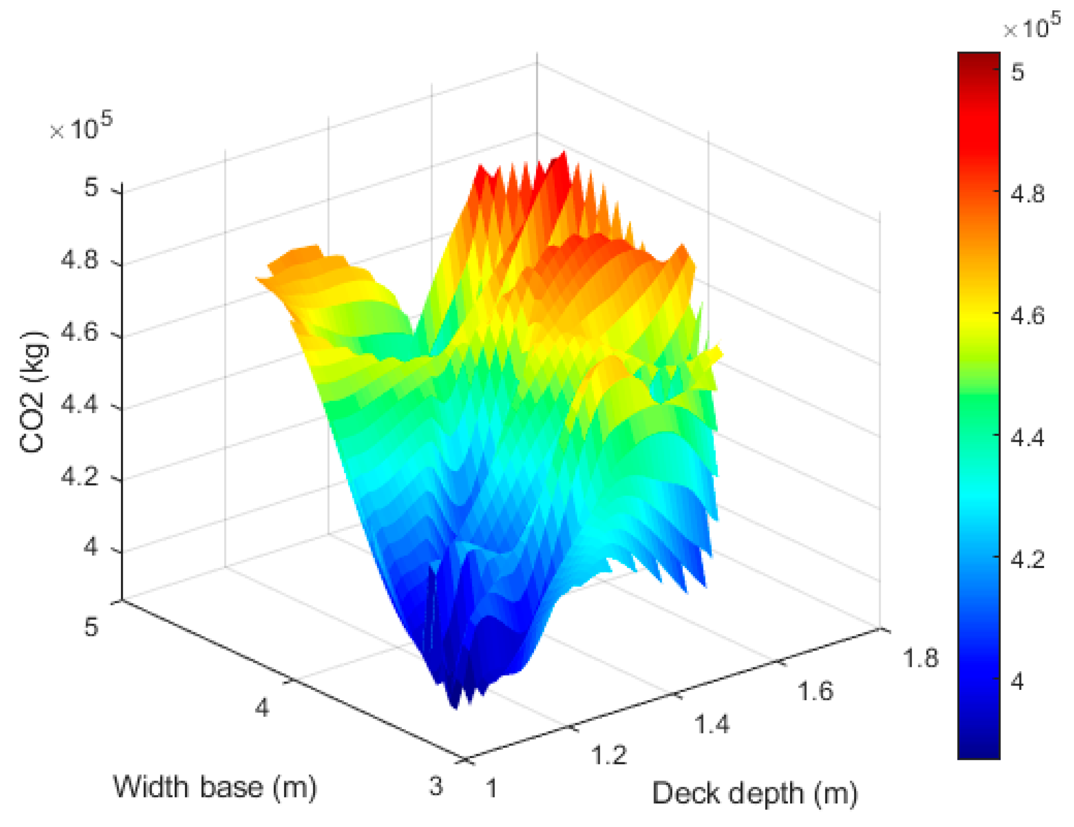
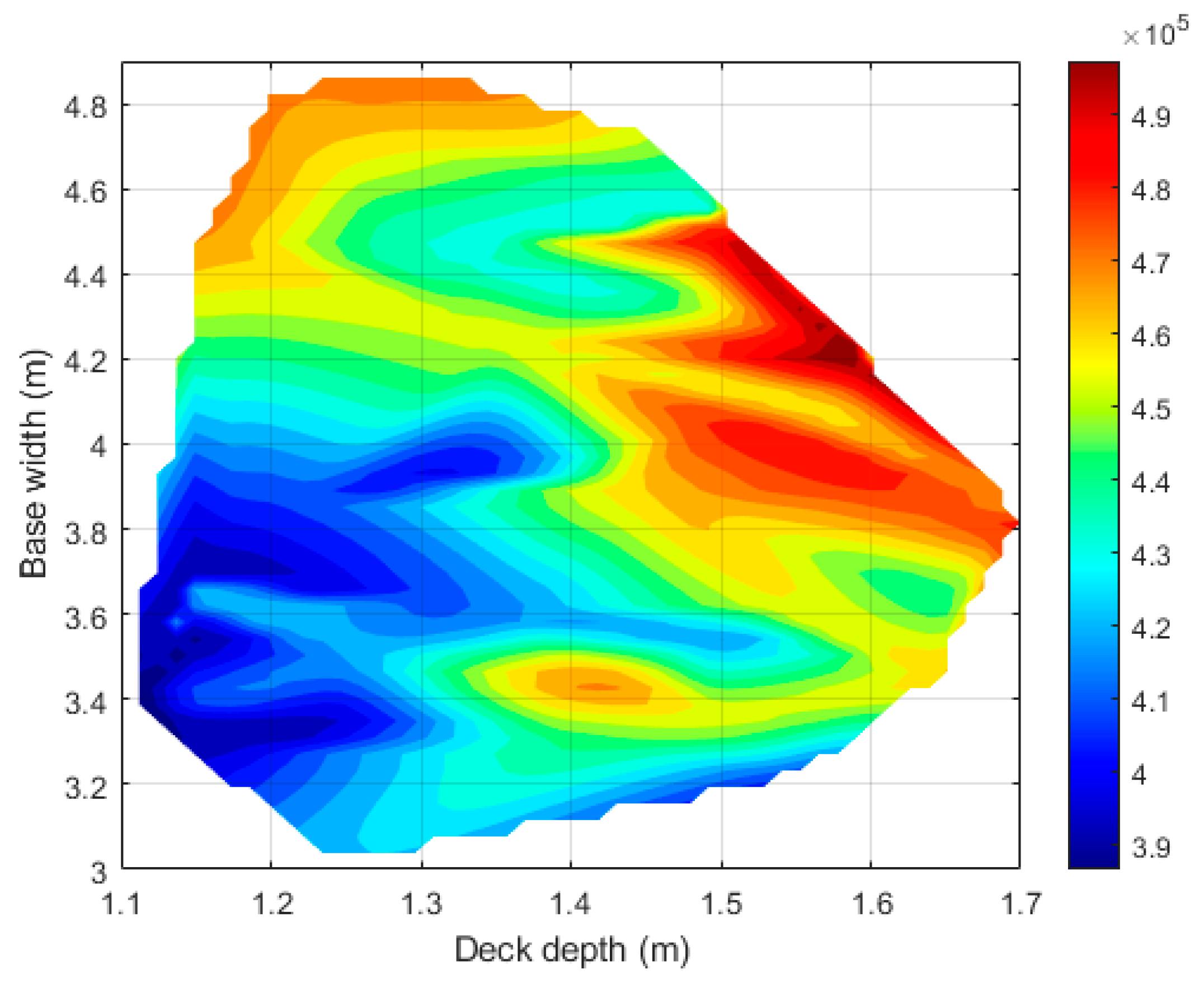
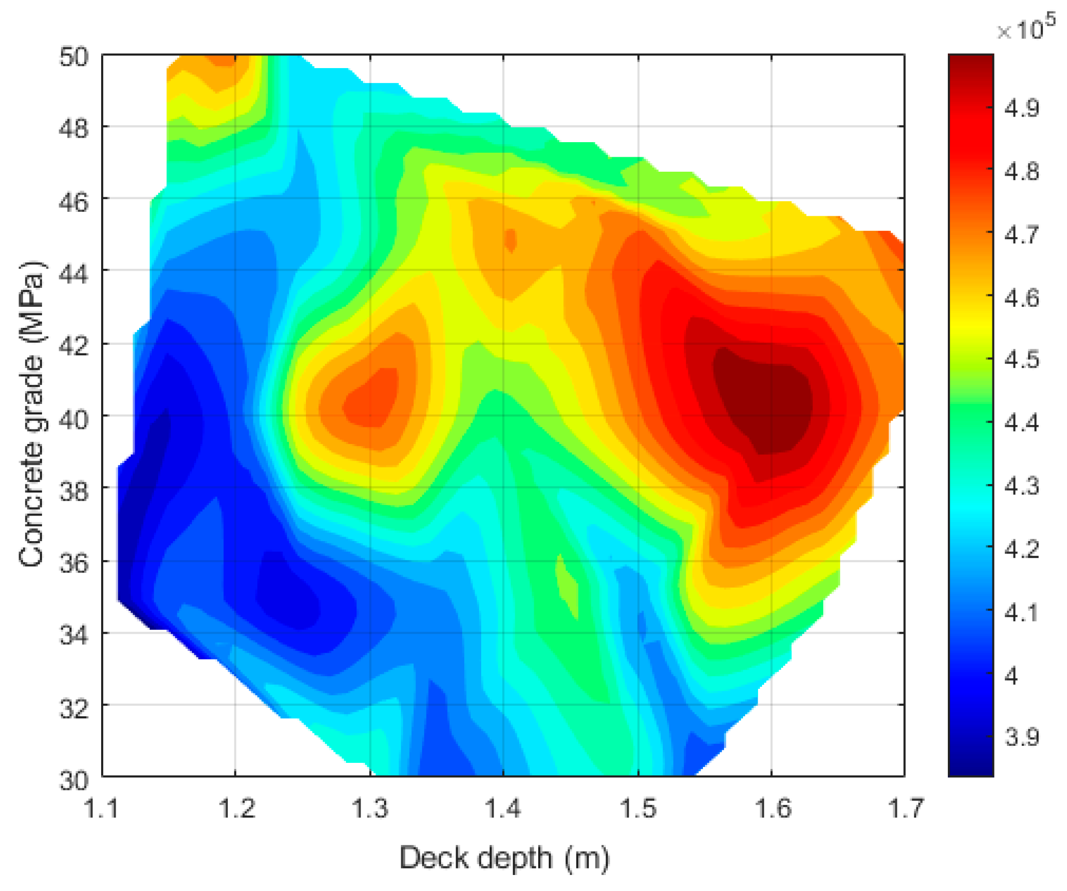
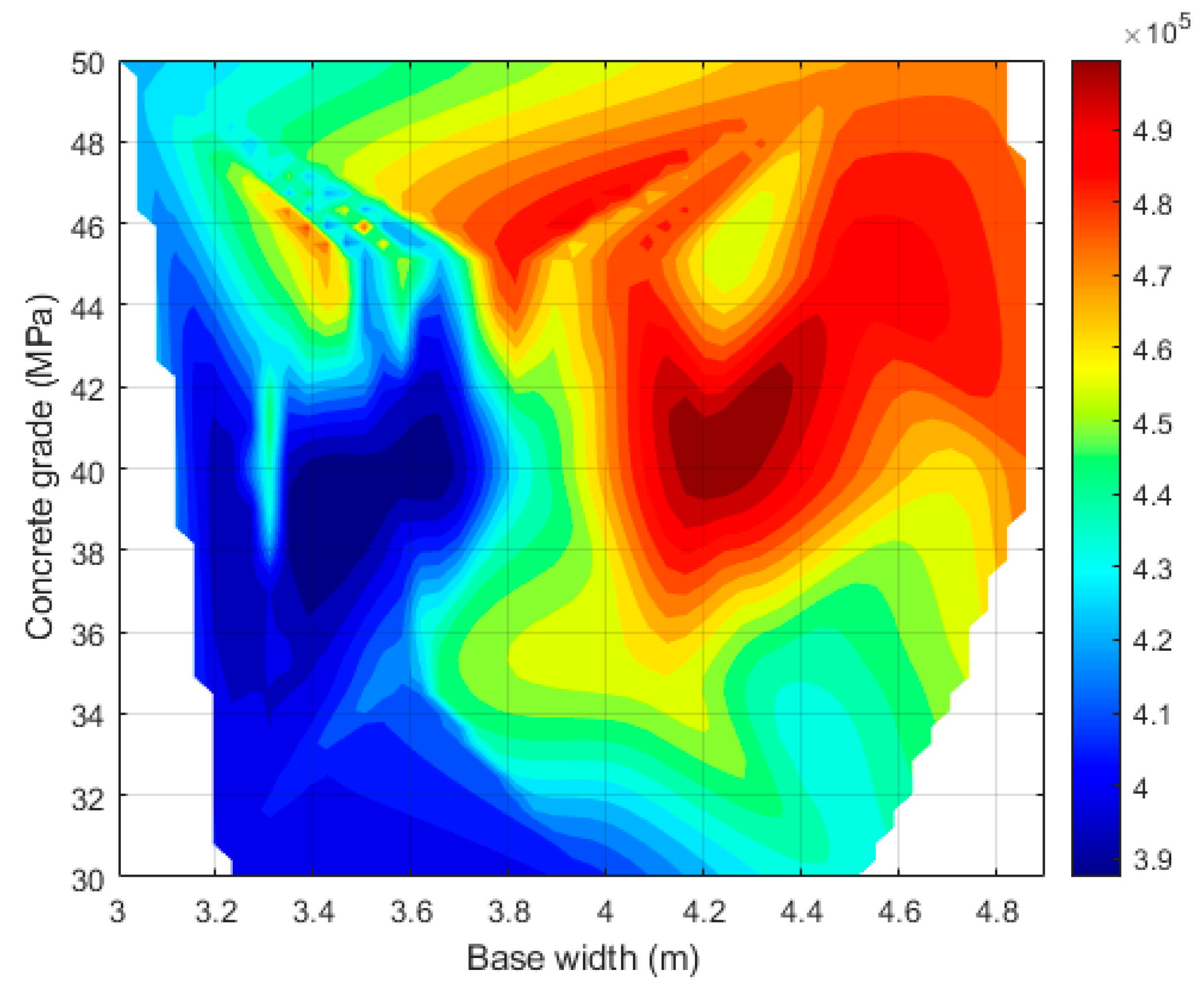
The observed data from Table 2 are represented in Figure 3, Figure 4, Figure 5 and Figure 6 with emissions as the output response, revealing multiple local optima and abruptness. A direct examination of Figure 3 shows that the lowest emissions are associated with the smallest base widths and deck depths within the specified ranges.
However, more detail regarding the location of the minimum emission values can be obtained by analyzing the contour plots representing the variables in pairs. Figure 4 demonstrates a two-dimensional representation of the response surface delineated in Figure 3, and a discernible trend is evident: a decline in CO2 emissions is concomitant with a reduction in base widths and deck depths.
As demonstrated in Figure 5, the maximum and minimum emission values are concentrated around the C-40 concrete grade, with deck depth playing a critical role. Specifically, within a deck depth range of 1.10 to 1.30 m and concrete grades between 35 and 40 MPa, the carbon footprint reaches its minimum.
Figure 6 shows that the maximum and minimum emission values are associated with C-40 concrete grade. The lowest carbon footprint is observed within a base width range of 3.20 to 3.80 m. Therefore, an initial assessment of the contour plots suggests that the lowest emissions can be achieved using concrete grades between 35 and 40 MPa, a deck depth of 1.10 to 1.30 m, and the width of the base between 3.20 and 3.80 m. These preliminary recommendations align with the optimum identified by optimizing the response surface generated using Kriging. This optimum, represented by deck #37, features the width of the base at 3.40 m, a deck depth of 1.10 m, and a C-35 concrete grade.

4. Discussion

4.1. Comparison with Previous Studies

The results obtained in this study are compared with those reported in previous research on similar types of bridges and with recommendations provided by other authors. Table 3 presents the key measurements of optimized bridges considering various objective functions such as cost [16] and embodied energy [15]. This study extends these optimization criteria by incorporating the reduction in CO2 emissions, thereby offering a more comprehensive approach to bridge design optimization. Table 3 also includes the reference bridge—the real-world constructed structure described in Section 2.1. This inclusion enables a direct comparison between the optimized designs and the reference one, offering important context to evaluate the practical relevance and effectiveness of the optimization approaches used in this study.
The slab height decreases notably from 1.35 m in the reference to 1.10 m in the CO2-optimized design, resulting in a higher span-to-depth ratio (30.91), which indicates a more slender and material-efficient structure. For prestressed slab bridges with cantilevers, recommended slenderness ratios provide benchmarks: The General Directorate of Public Roads of Spain [50] suggests 1/22 to 1/30, SETRA [51] 1/28, and Manterola [52] 1/25. The reference bridge’s slenderness (1/25.19) fits these ranges. The cost-optimized bridge is less slender than CO2 and energy-optimized versions, implying cost-effectiveness at slenderness above 1/26 and sustainability goals near 1/30.
Concrete volume reduces accordingly, reaching 0.56 m3/m2 in the CO2 case, lowering the embodied carbon footprint. However, the reduced slab depth requires increased passive steel reinforcement (77.00 kg/m2) to maintain flexural strength, while active steel remains stable, indicating prestressing is driven mainly by structural needs. The cost-driven design balances material savings with feasibility, showing moderate reductions in slab height and concrete volume with minimal changes in steel. The energy-optimized solution lowers passive steel (69.41 kg/m2), likely reflecting steel’s higher embodied energy, favoring concrete within structural limits. These differences highlight trade-offs between efficiency, material properties, and sustainability, with CO2 optimization favoring aggressive material cuts and increased steel, while cost and energy targets yield balanced solutions.

4.2. Surrogate Model Performance

Table 4 presents the real values alongside results from three Kriging surrogate models, a linear regression, and the local optimum obtained from the ANN’s diversification (#36) and intensification (#37) phases. While the Kriging models are deterministic, ANNs and GPR are inherently stochastic due to random training and validation splits. To account for this variability, each configuration was run 16 times with different random seeds, reducing the standard error of the mean and yielding more robust predictions. Mean values of each performance metric are reported, and the 95% confidence intervals for RMSE and MAE overlap, indicating no statistically significant differences between models. Early stopping on the validation set was applied to every run to limit overfitting.
The prediction of the 30 slabs used in the diversification phase was compared for all models (Table 1) to analyze the relative error. The linear model provides the lowest relative error concerning the optimum of the intensification phase. However, the scenario changes when examining the RMSE, RSR, and MAE for the prediction of slabs #31 to #37, as summarized in Table 5, which also includes an added ranking column (‘Rank (RMSE→MAE→RSR)’) to facilitate model selection. Models are ordered primarily by RMSE (lower is better), with MAE and RSR as tie-breakers when RMSE differences are slight. It can be observed that the neural network achieves the lowest RMSEs, closely followed by the Kriging 1 model.
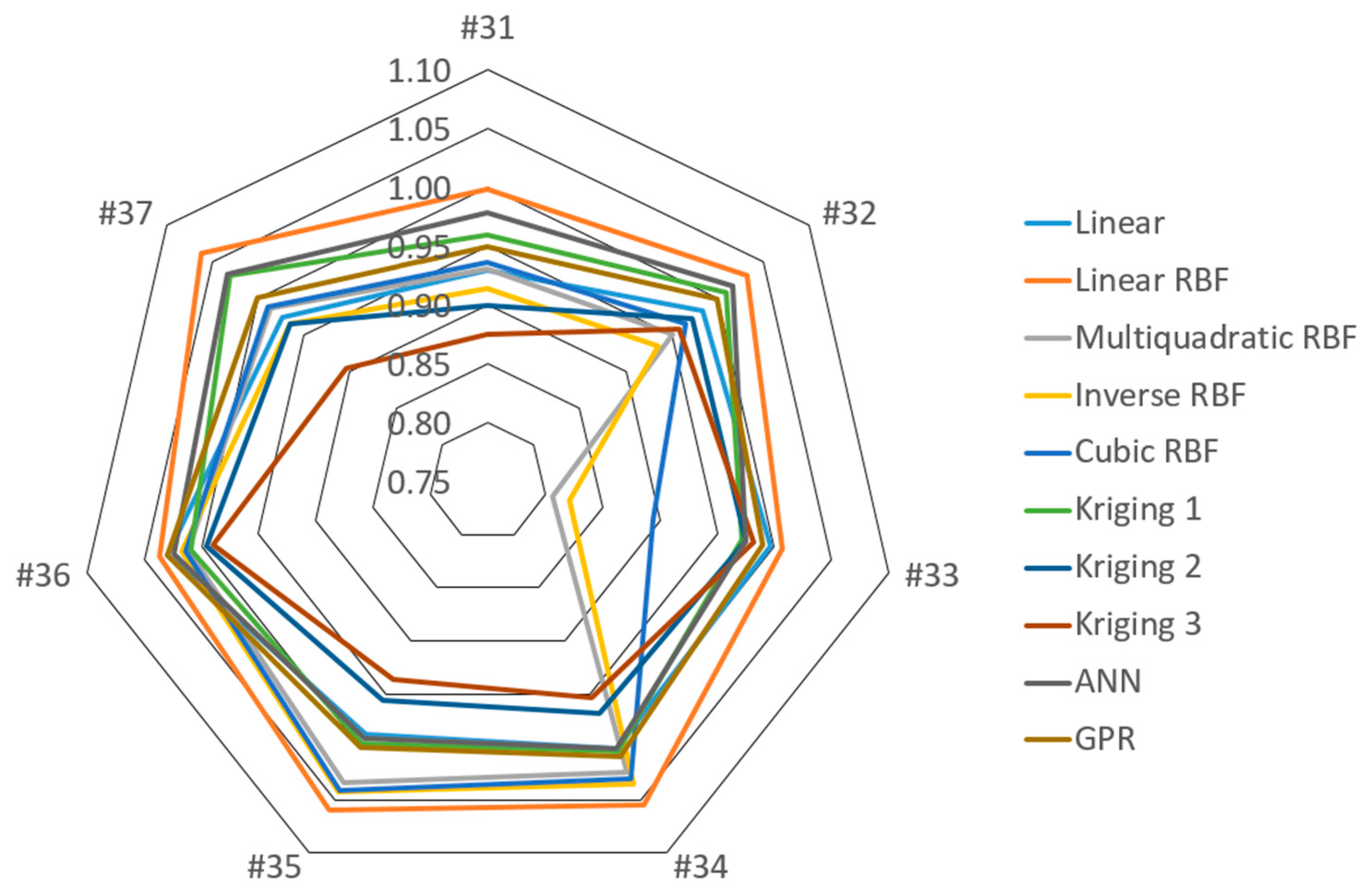
Figure 7 illustrates the predicted-to-real values for points #31 to #37 across the metamodels. The prediction improves as the ratio approaches one. It can be observed that Kriging 2 and Kriging 3 tend to underestimate the predicted values. In contrast, Kriging 1, ANN, and GPR models achieve ratios closest to unity on average.
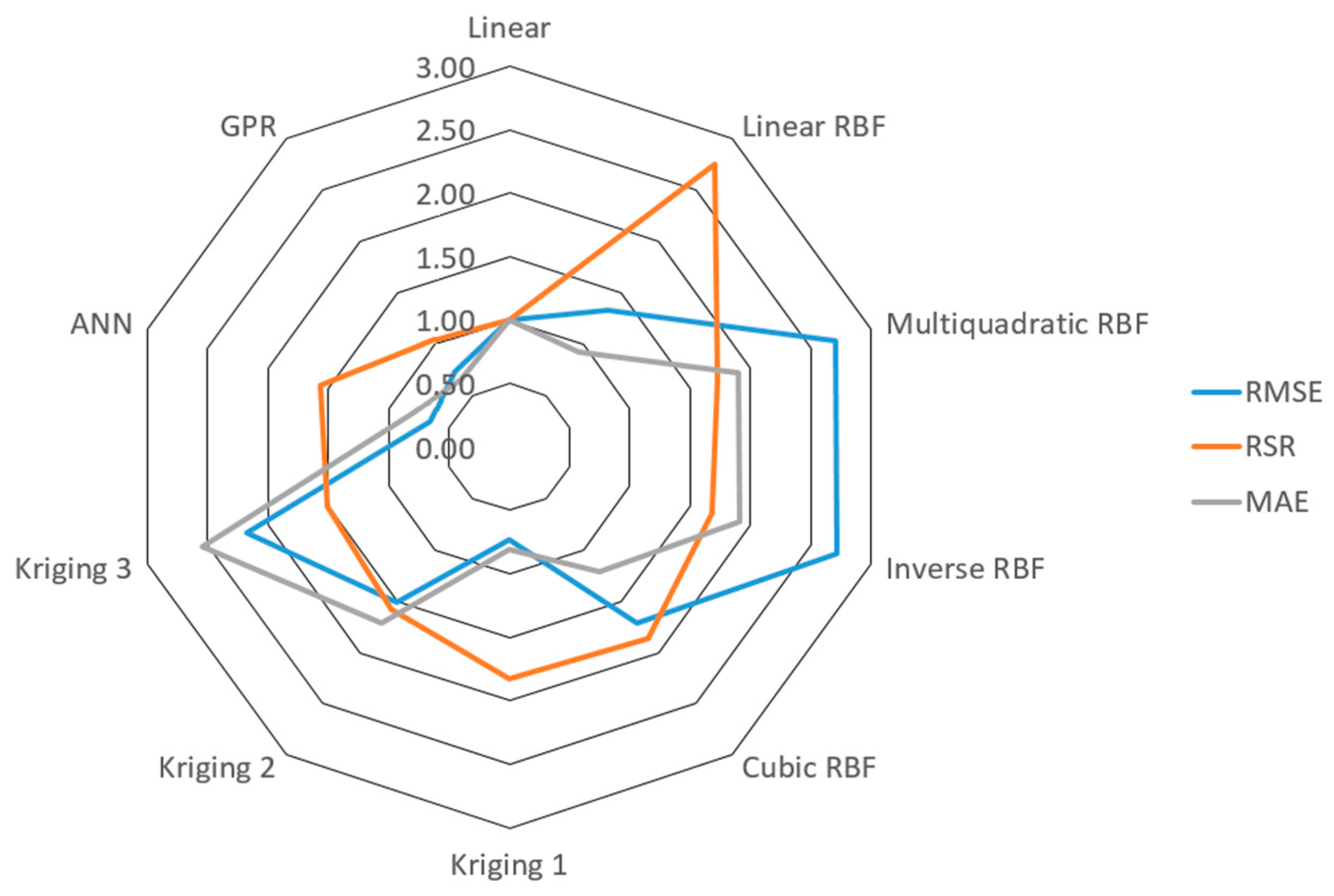
Figure 8 displays the metrics used to evaluate the effectiveness of each predictive model in this research. The values have been divided by the metrics of the linear model to allow for comparison of the normalized values. A lower metric value indicates improved predictive reliability of the model. The ANN and GPR models exhibit the best performance.
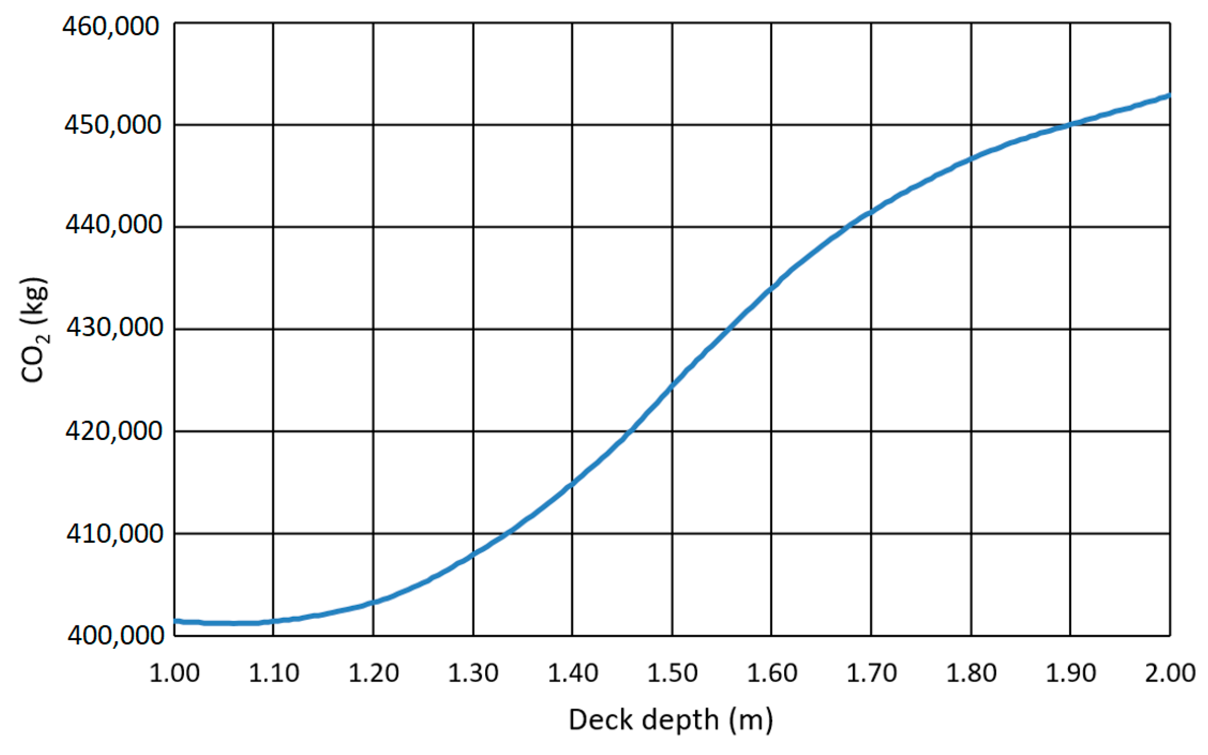
The ability of the ANN to identify optimal values is evaluated by analyzing the averages of 16 runs with the 37 observed values. Figure 9 predicts the minimum deck depth for a width of the base of 3.40 m and a concrete grade of C35. The optimal deck depth obtained with Kriging, 1.10 m, coincides with the neural network results, which indicate an increase in CO2 emissions from this measure. This confirms the consistency between the two approaches to optimization.
With C35 concrete and a deck depth of 1.10 m, the ANN illustrates the variation in emissions as the deck width changes. Emissions are minimal between the 3.00 m and 3.40 m base, rising slowly thereafter and more steeply from 4.00 m onwards (Figure 10). This is consistent with the minimum base value found when optimizing the Kriging response surface, which was 3.40 m.
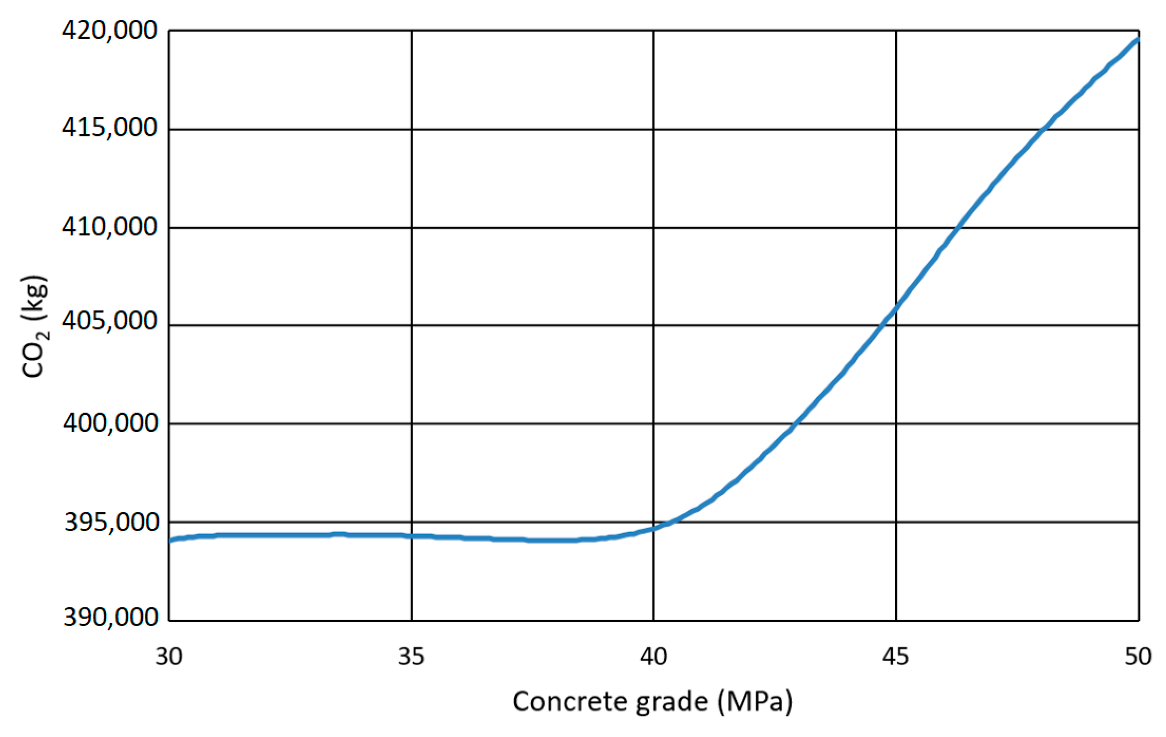
If the deck depth is now kept at 1.10 m and the base at 3.40 m, the neural network shows how CO2 emissions evolve with the characteristic strength of the concrete (Figure 11). From 30 to 40 MPa, emissions remain at their lowest values, clearly increasing thereafter. This agrees with the value of 35 MPa obtained from the response surface optimization generated by the Kriging metamodel.

4.3. Practical Design Recommendations

The General Directorate of Public Roads of Spain [50] suggests a ratio between the depth of the deck and the main span length ranging from 1/22 and 1/30, whereas SETRA [51] advocates a value of 1/28 particularly for PC decks composed of three-span with wide lateral cantilever lengths. The ANN results guide the practical minimization of the carbon footprint in a PC deck with a 34 m main span. It is recommended to aim for the highest possible slenderness ratios, preferably within the range of 1/30, which would necessitate an increase in passive steel. Decreasing the concrete and active steel volume can compensate for this additional passive reinforcement. Additionally, the amount of lightening should be maximized to minimize concrete use further.
The following design guidelines are recommended for a PC road flyover with a main span of 34 m: a depth/span ratio exceeding 1/28, a concrete volume below 0.60 m3/m2 of deck, and passive reinforcement above 120 kg/m3 of concrete. Active steel should remain under 17 kg/m2 of the deck. The recommended concrete grade ranges between 35 and 40 MPa. The external voids should range from 0.40 to 0.50 m3/m2, while the internal voids should be lower than 0.20 m3/m2.
The ANN can identify a local optimum that closely aligns with the Kriging response surface local optimum. Nevertheless, to predict CO2 emissions with higher accuracy, a heuristic optimization process must be applied to both Kriging models and ANN. While metamodels can effectively generate a response surface, minimizing it to locate a local minimum is crucial. Despite this, these models offer reliable project outcomes and significantly contribute to refining the definition of suitable value intervals for key design variables. The methodology is a valuable tool for designers who may not regularly employ heuristic optimization algorithms, thus enabling them to uncover potential opportunities for reducing economic costs and carbon footprint.

4.4. Limitations and Future Work

The present study provides a consistent and well-founded framework for optimizing the carbon footprint of prestressed lightweight slab bridges. Nonetheless, several aspects naturally suggest future research avenues beyond the current scope. The methodology was illustrated through a representative case study; its application to alternative bridge typologies would broaden the range of structural configurations addressed. Although the surrogate models and optimization strategies were carefully selected and calibrated, further enhancements could be achieved by incorporating larger datasets. Hybrid optimization schemes—combining heuristic search with surrogate-assisted refinement—can improve solution accuracy by exploiting the global exploration capacity of heuristics and the local precision of surrogate models, thereby reducing computational effort while increasing reliability.
Furthermore, integrating multi-objective formulations that balance CO2 emissions with cost, structural performance, and constructability would provide a more comprehensive decision-making framework. The assessment of innovative materials, such as high-performance or low-carbon concretes, recycled aggregates, and advanced reinforcement systems, is expected to reduce embodied emissions and enhance durability and service life, amplifying long-term sustainability gains. Finally, incorporating life-cycle assessment to capture use-phase and end-of-life effects, together with validation through real construction projects, would strengthen the practical relevance and robustness of the methodology. These extensions represent natural continuations of the present work and hold significant potential to advance sustainable and efficient bridge engineering.

5. Concluding Remarks

This study compares Kriging and artificial neural networks (ANNs) for optimizing the carbon footprint in prestressed slab bridge design. The research uses Latin hypercube sampling (LHS) and two-phase optimization to identify key design parameters—deck depth, base width, and concrete grade—influencing CO2 emissions. ANNs show superior predictive accuracy, outperforming other models in reducing RMSE and MAE. Verification indicates that neural networks effectively identify the local optimum, closely resembling values obtained by minimizing the Kriging response surface. Nevertheless, neither model accurately predicts the objective function and guides solutions toward promising areas. While these models closely define a response surface, refining the optimization to locate a more precise local minimum remains necessary. Optimal configurations include concrete grades between C-35 and C-40 MPa, deck depths from 1.10 to 1.30 m, and base widths from 3.20 to 3.80 m, highlighting the role of advanced surrogate models in sustainable bridge engineering.
This study provides practical recommendations, advocating for slenderness ratios above 1/28, concrete volumes below 0.60 m3/m2, passive reinforcement over 120 kg/m3, and prestressing reinforcement under 17 kg/m2. Enhanced lightening strategies, including external voids of 0.40 to 0.50 m3/m2 and internal voids below 0.20 m3/m2, further improve sustainability. ANN-based optimization enables eco-efficient designs while ensuring structural integrity. This methodology is a practical tool for identifying optimal configurations without excessive computational costs, bridging theoretical advancements with real-world applications.
Beyond its technical contributions, this study has potential impacts across research, economic, and sustainability domains. From a research perspective, it adds comparative evidence on the performance of surrogate models in structural optimization when working with small datasets. Economically, it supports identifying design configurations that simultaneously reduce costs and embodied CO2. Societally and in terms of sustainability, it facilitates adopting environmentally friendly bridge design practices, contributing to greener and more responsible infrastructure development.

Author Contributions

This paper represents the result of teamwork. Conceptualization, L.Y.-B. and V.Y.; methodology, L.Y.-B. and V.Y.; software, L.Y.-B. and J.A.; validation, L.Y.-B. and J.A.; formal analysis, L.Y.-B. and J.A.; investigation, L.Y.-B., J.A. and V.Y.; resources, V.Y.; data curation, L.Y.-B.; writing—original draft preparation, L.Y.-B.; writing—review and editing, V.Y.; visualization, L.Y.-B.; supervision, J.A. and V.Y.; project administration, V.Y.; funding acquisition, V.Y. All authors have read and agreed to the published version of the manuscript.

Funding

This research was funded by Grant PID2023-150003OB-I00 funded by MCIN/AEI/10.13039/501100011033 and by “ERDF A way of making Europe”.

Institutional Review Board Statement

Not applicable.

Informed Consent Statement

Not applicable.

Data Availability Statement

Data are contained within the article.

Conflicts of Interest

The authors declare no conflicts of interest.

References

  1. Alhorr, Y.; Eliskandarani, E.; Elsarrag, E. Approaches to reducing carbon dioxide emissions in the built environment: Low carbon cities. Int. J. Sustain. Built Environ. 2014, 3, 167–178. [Google Scholar] [CrossRef]
  2. World Green Building Council (WGBC). How We Are #Building the Transition to Support the Sustainable Development Goals. 2023. Available online: https://worldgbc.org/wp-content/uploads/2023/09/Buildings-SDG-graphic-1.pdf (accessed on 23 July 2025).
  3. Gursel, A.P.; Masanet, E.; Horvath, A.; Stadel, A. Life-cycle inventory analysis of concrete production: A critical review. Cem. Concr. Compos. 2014, 51, 38–48. [Google Scholar] [CrossRef]
  4. Opoku, D.G.J.; Agyekum, K.; Ayarkwa, J. Drivers of environmental sustainability of construction projects: A thematic analysis of verbatim comments from built environment consultants. Int. J. Constr. Manag. 2022, 22, 1033–1041. [Google Scholar] [CrossRef]
  5. Halder, A.; Batra, S. Application of predictive analytics in built environment research: A comprehensive bibliometric study to explore knowledge domains and future research agenda. Arch. Comput. Methods Eng. 2023, 30, 4299–4324. [Google Scholar] [CrossRef]
  6. Salah, M.; Alabdullatief, A. Architecture of tomorrow: The construction industry in the era of artificial intelligence. Autom. Constr. 2025, 178, 106429. [Google Scholar] [CrossRef]
  7. Cabeza, L.F.; Boquera, L.; Chàfer, M.; Vérez, D. Embodied energy and embodied carbon of structural building materials: Worldwide progress and barriers through literature map analysis. Energy Build. 2021, 231, 110612. [Google Scholar] [CrossRef]
  8. Hasan, S.M.; Mashud, A.H.M.; Miah, S.; Daryanto, Y.; Lim, M.K.; Tseng, M.L. A green inventory model considering environmental emissions under carbon tax, cap-and-offset, and cap-and-trade regulations. J. Ind. Prod. Eng. 2023, 40, 538–553. [Google Scholar] [CrossRef]
  9. Konstandakopoulou, F.; Tsimirika, M.; Pnevmatikos, N.; Hatzigeorgiou, G.D. Optimization of reinforced concrete retaining walls designed according to European provisions. Infrastructures 2020, 5, 46. [Google Scholar] [CrossRef]
  10. Sun, G.; Wang, Y.; Yang, J.; Chen, S.; Liu, H.; Zhao, J. Lightweight design method of orthotropic steel bridge deck with U-ribs based on multi-objective optimization. Ain Shams Eng. J. 2024, 15, 102414. [Google Scholar] [CrossRef]
  11. Mashud, A.H.M.; Roy, D.; Chakrabortty, R.K.; Tseng, M.L.; Pervin, M. An optimum balance among the reduction in ordering cost, product deterioration and carbon emissions: A sustainable green warehouse. Environ. Sci. Pollut. Res. 2022, 29, 78029–78051. [Google Scholar] [CrossRef] [PubMed]
  12. Ni, W.; Shu, J. Trade-off between service time and carbon emissions for safety stock placement in multi-echelon supply chains. Int. J. Prod. Res. 2015, 53, 6701–6718. [Google Scholar] [CrossRef]
  13. Hassanzadeh, A.; Moradi, S.; Burton, H.V. Performance-Based Design Optimization of Structures: State-of-the-Art Review. J. Struct. Eng. 2024, 150, 03124001. [Google Scholar] [CrossRef]
  14. Martínez-Frutos, J.; Martí, P. Robust design optimization using Kriging models: Application to the robust design optimization of truss structures. Rev. Int. Métodos Numér. Cálc. Diseño Ing. 2014, 30, 97–105. [Google Scholar] [CrossRef]
  15. Yepes-Bellver, L.; Brun-Izquierdo, A.; Alcalá, J.; Yepes, V. Embodied energy optimization of prestressed concrete road flyovers by a two-phase Kriging surrogate model. Materials 2023, 16, 6767. [Google Scholar] [CrossRef]
  16. Yepes-Bellver, L.; Brun-Izquierdo, A.; Alcalá, J.; Yepes, V. Surrogate-assisted cost optimization for post-tensioned concrete slab bridges. Infrastructures 2025, 10, 43. [Google Scholar] [CrossRef]
  17. YiFei, L.; MaoSen, C.; Hoa, T.N.; Khatir, S.; Minh, H.L.; SangTo, T.; Cuong-Le, T.; Wahab, M.A. Metamodel-assisted hybrid optimization strategy for model updating using vibration response data. Adv. Eng. Softw. 2023, 185, 103515. [Google Scholar] [CrossRef]
  18. Sánchez-Zabala, V.F.; Gómez-Acebo, T. Building energy performance metamodels for district energy management optimization platforms. Energy Convers. Manag. X 2024, 21, 100512. [Google Scholar] [CrossRef]
  19. Neto, T.F.C.; Cascudo, O. Prediction of natural carbonation depths in concretes with ensemble metamodel based on artificial neural networks from time series analysis with 20 years of exposure. J. Build. Eng. 2025, 111, 113352. [Google Scholar] [CrossRef]
  20. Martí-Vargas, J.R.; Ferri, F.J.; Yepes, V. Prediction of the transfer length of prestressing strands with neural networks. Comput. Concr. 2013, 12, 187–209. [Google Scholar] [CrossRef]
  21. Nayak, S.C.; Dehuri, S.; Cho, S.B. An evolutionary functional link artificial neural network for assessment of compressive strength of concrete structures. Ain Shams Eng. J. 2024, 15, 102462. [Google Scholar] [CrossRef]
  22. Zheng, S.; Li, Z.; Wang, H. A Genetic Fuzzy Radial Basis Function Neural Network for Structural Health Monitoring of Composite Laminated Beams. Expert Syst. Appl. 2011, 38, 11837–11842. [Google Scholar] [CrossRef]
  23. Machavaram, R.; Shankar, K. Structural Damage Identification Using Improved RBF Neural Networks in Frequency Domain. Adv. Struct. Eng. 2012, 15, 1689–1703. [Google Scholar] [CrossRef]
  24. Saida, T.; Rashid, M.; Nishio, M. System Fragility Analysis of Highway Bridge Using Multi-Output Gaussian Process Regression Surrogate Model. Adv. Struct. Eng. 2024, 27, 2803–2822. [Google Scholar] [CrossRef]
  25. da Silva, S.; Figueiredo, E.; Moldovan, I. Damage Detection Approach for Bridges under Temperature Effects Using Gaussian Process Regression Trained with Hybrid Data. J. Bridge Eng. 2022, 27, 04022107. [Google Scholar] [CrossRef]
  26. Yepes, V.; Martí, J.V.; García-Segura, T. Cost and CO2 emission optimization of precast-prestressed concrete U-beam road bridges by a hybrid glowworm swarm algorithm. Automation Constr. 2015, 49, 123–134. [Google Scholar] [CrossRef]
  27. García-Segura, T.; Yepes, V.; Alcalá, J.; Pérez-López, E. Hybrid harmony search for sustainable design of post-tensioned concrete box-girder pedestrian bridges. Eng. Struct. 2015, 92, 112–122. [Google Scholar] [CrossRef]
  28. García-Segura, T.; Yepes, V. Multiobjective optimization of post-tensioned concrete box-girder road bridges considering cost, CO2 emissions, and safety. Eng. Struct. 2016, 125, 325–336. [Google Scholar] [CrossRef]
  29. Suwondo, R.; Keintjem, M.; Suangga, M.; Cunningham, L. Assessing embodied carbon and financial implications in concrete T-girder bridge design for cost-effective sustainability. Innov. Infrastruct. Solut. 2024, 9, 136. [Google Scholar] [CrossRef]
  30. Penadés-Plà, V.; García-Segura, T.; Martí, J.V.; Yepes, V. An optimization-LCA of a prestressed concrete precast bridge. Sustainability 2018, 10, 685. [Google Scholar] [CrossRef]
  31. Kim, B.-S.; Lee, Y.-B.; Choi, D.-H. Comparison study on the accuracy of metamodeling technique for non-convex functions. J. Mech. Sci. Technol. 2009, 23, 1175–1181. [Google Scholar] [CrossRef]
  32. Li, Y.F.; Ng, S.H.; Xie, M. A systematic comparison of metamodeling techniques for simulation optimization in decision support systems. Appl. Soft Comput. 2010, 10, 1257–1273. [Google Scholar] [CrossRef]
  33. Ryberg, A. Metamodel-Based Design Optimization—A Multidisciplinary Approach for Automotive Structures. 2013. Available online: https://liu.diva-portal.org/smash/get/diva2:601789/FULLTEXT01.pdf (accessed on 19 June 2025).
  34. Jin, R.; Chen, W.; Simpson, T. Comparative studies of metamodelling techniques under multiple modelling criteria. Struct. Multidiscip. Optim. 2001, 23, 1–13. [Google Scholar] [CrossRef]
  35. Elwy, I.; Hagishima, A. The artificial intelligence reformation of sustainable building design approach: A systematic review on building design optimization methods using surrogate models. Energy Build. 2024, 323, 114769. [Google Scholar] [CrossRef]
  36. Catalonia Institute of Construction Technology. BEDEC PR/PCT ITEC Materials Database. Barcelona, Spain. Available online: http://www.itec.cat (accessed on 29 January 2025).
  37. Lophaven, N.S.; Nielsen, H.B.; Søndergaard, J. MATLAB Kriging Toolbox DACE (Design and Analysis of Computer Experiments) Version 2.0. 2002. Available online: http://www2.imm.dtu.dk/pubdb/p.php?1460 (accessed on 22 May 2025).
  38. McKay, M.D.; Beckman, R.J.; Conover, W.J. A comparison of three methods for selecting values of input variables in the analysis of output from a computer code. Technometrics 1979, 21, 239–245. [Google Scholar] [CrossRef]
  39. Buhmann, M.D. Radial basis functions. Acta Numer. 2000, 9, 1–38. [Google Scholar] [CrossRef]
  40. Cressie, N. The origins of Kriging. Math. Geol. 1990, 22, 239–252. [Google Scholar] [CrossRef]
  41. LeCun, Y.; Bengio, Y.; Hinton, G. Deep learning. Nature 2015, 521, 436–444. [Google Scholar] [CrossRef]
  42. Zhang, G.; Patuwo, B.E.; Hu, M.Y. Forecasting with artificial neural networks: The state of the art. Int. J. Forecast. 1998, 14, 35–62. [Google Scholar] [CrossRef]
  43. Hornik, K.; Stinchcombe, M.; White, H. Multilayer feedforward networks are universal approximators. Neural Netw. 1989, 2, 359–366. [Google Scholar] [CrossRef]
  44. Rumelhart, D.E.; McClelland, J.L.; PDP Research Group. Parallel Distributed Processing: Explorations in the Microstructure of Cognition. Volume 1: Foundations; MIT Press: Cambridge, UK, 1986. [Google Scholar] [CrossRef]
  45. Rumelhart, D.E.; Hinton, G.E.; Williams, R.J. Learning representations by back-propagating errors. Nature 1986, 323, 533–536. [Google Scholar] [CrossRef]
  46. Beale, M.H.; Hagan, M.T.; Demuth, H.B. Neural Network Toolbox User’s Guide; The MathWorks: Natick, MA, USA, 2017; p. 512. [Google Scholar]
  47. Schulz, E.; Speekenbrink, M.; Krause, A. A tutorial on Gaussian process regression: Modelling, exploring, and exploiting functions. J. Math. Psychol. 2018, 85, 1–16. [Google Scholar] [CrossRef]
  48. Satria Palar, P.; Rizki Zuhal, L.; Shimoyama, K. Gaussian process surrogate model with composite kernel learning for engineering design. AIAA J. 2020, 58, 1864–1880. [Google Scholar] [CrossRef]
  49. Kianifar, M.R.; Campean, F. Performance evaluation of metamodelling methods for engineering problems: Towards a practitioner guide. Struct. Multidiscip. Optim. 2020, 61, 159–186. [Google Scholar] [CrossRef]
  50. Dirección General de Carreteras. Obras de Paso de Nueva Construcción: Conceptos Generales; Ministerio de Fomento, Centro de Publicaciones: Madrid, Spain, 2000. [Google Scholar]
  51. SETRA. Ponts-Dalles. Guide de Conception; Ministère de l’Équipement, du Logement des Transports et de la Mer: Paris, France, 1989. [Google Scholar]
  52. Manterola, J. Puentes: Apuntes para su Diseño, Cálculo y Construcción; Colegio de Ingenieros de Caminos, Canales y Puertos: Madrid, Spain, 2006. [Google Scholar]
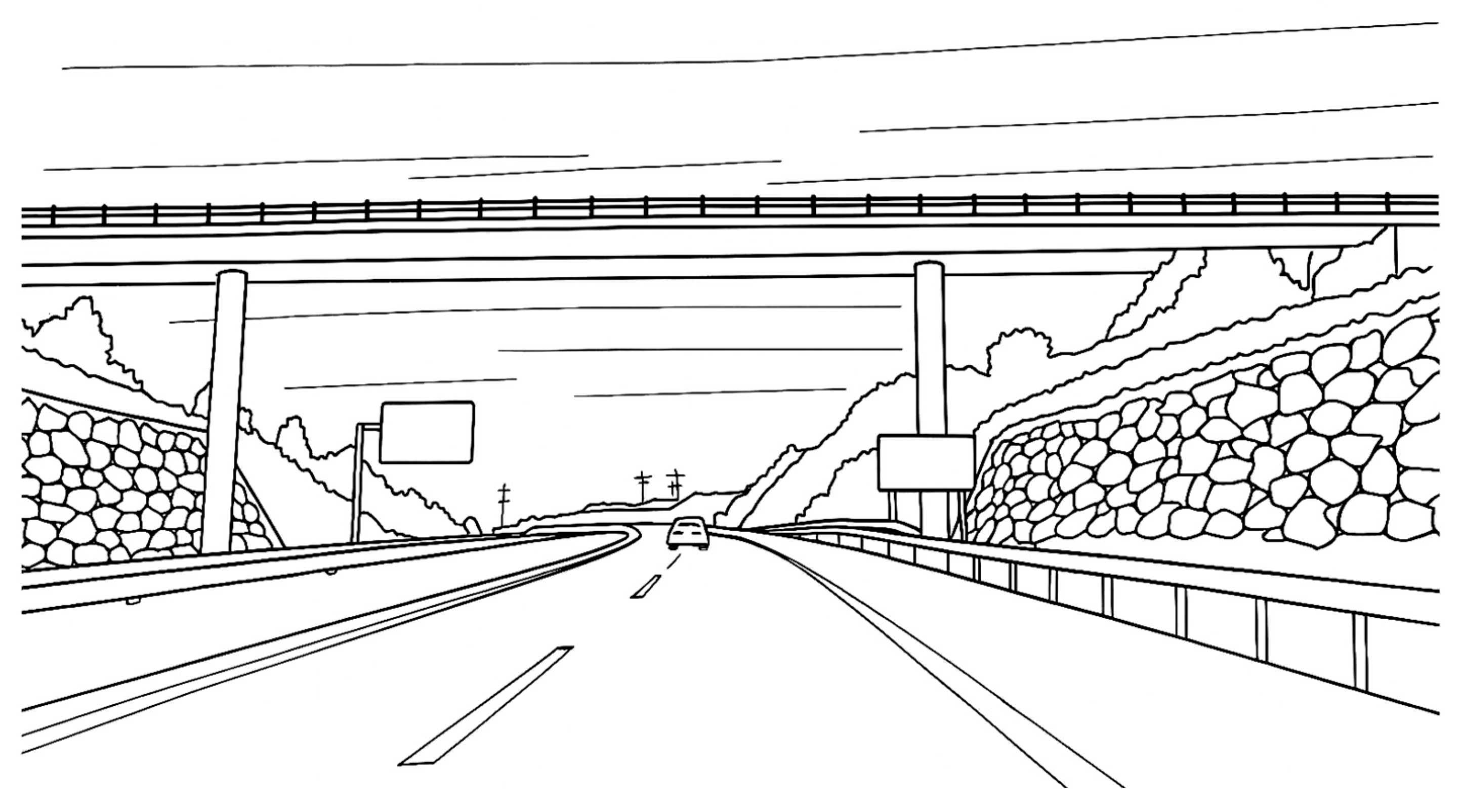
Figure 1. Longitudinal view of the lightweight PC slab.
Applsci 15 09591 g001
Figure 2. Bridge deck cross-section of the lightweight PC slab.
Applsci 15 09591 g002
Figure 3. Response surface corresponding to the 37 slab bridge decks.
Applsci 15 09591 g003
Figure 4. Contour plot showing emissions based on deck depth and base width (Table 2).
Applsci 15 09591 g004
Figure 5. Contour plot showing emissions based on deck depth and concrete grade (Table 2).
Applsci 15 09591 g005
Figure 6. Contour plot showing emissions based on base width and concrete grade (Table 2).
Applsci 15 09591 g006
Figure 7. Ratio between predicted and observed data for decks #31 to #37. Ratios closer to 1 indicate better agreement between predicted and observed values.
Applsci 15 09591 g007
Figure 8. Model performance metrics normalized to the linear model. Lower ratio values indicate smaller errors in the predictive models.
Applsci 15 09591 g008
Figure 9. ANN prediction of CO2 based on deck depth, considering a base width of 3.40 m and a concrete compressive strength of 35 MPa.
Applsci 15 09591 g009
Figure 10. ANN prediction of CO2 based on the base width (1.10 m deck depth and 35 MPa concrete grade).
Applsci 15 09591 g010
Figure 11. ANN prediction of CO2 based on the concrete grade (1.10 m deck depth and 3.40 m base width).
Applsci 15 09591 g011
Table 1. Deck unit costs.
Deck UnitUnitCO2 (kg)
C-30 concretem3227.01
C-35 concretem3263.96
C-40 concretem3298.57
C-45 concretem3330.25
C-50 concretem3358.97
Steel reinforcementkg3.03
Steel prestressedkg5.64
Formworkm22.24
Voidsm3604.42
Table 2. Data derived from calculated bridges.
DeckDeck Depth
(m)
Base Width
(m)
Concrete Grade
(MPa)
CO2
(kg)
11.454.3535439,416
21.554.1035460,393
31.454.7535455,722
41.703.8045484,897
51.203.8540407,988
61.553.6045456,668
71.204.8550472,401
81.154.5050471,362
91.353.9530406,654
101.304.4530436,703
111.354.2545455,374
121.504.5530434,674
131.604.2040503,797
141.254.7040462,915
151.504.0545482,659
161.304.9040477,491
171.653.6535444,714
181.653.4545464,051
191.253.5045420,514
201.403.3040443,840
211.453.9045464,536
221.353.6035416,584
231.503.3545455,442
241.504.5045490,669
251.553.2030403,972
261.253.0050423,112
271.403.4545470,008
281.503.5535418,839
291.703.8540468,898
301.153.7040394,616
311.153.4035411,077
321.253.3535398,614
331.153.6545422,934
341.153.3540395,465
351.153.2540397,154
361.153.5540391,370
371.103.4035386,515
Table 3. Measurements of the reference deck and the optimized solutions.
Objective FunctionSlab Height (m)Span/Deck DepthConcrete (m3/m2)Passive Steel (kg/m2)Active Steel (kg/m2)
Reference1.3525.190.7273.4516.64
Cost1.3026.150.6173.5314.76
CO21.1030.910.5677.0016.48
Energy1.1529.570.6169.4116.65
Table 4. Real values and predictions corresponding to the optimal solutions identified during the diversification phase (#36) and the intensification phase (#37), along with their relative errors.
Local OptimaRelative Error (%)
#36#37#36#37
Observed391,370386,5150.000.00
Linear402,802376,5712.92−2.57
Linear RBF405,515410,2173.616.13
Multiquadratic RBF395,904381,2081.16−1.37
Inverse multiquadratic RBF397,924373,2581.67−3.43
Cubic RBF396,853382,2251.40−1.11
Kriging 1394,808398,4960.883.10
Kriging 2389,612373,195−0.45−3.45
Kriging 3387,247349,638−1.05−9.54
ANN average400,619399,2192.363.29
GPR average403,150386,8803.010.09
Table 5. Used prediction model error metrics.
Predictive ModelsRMSE RSRMAERank (RMSE-RSR-MAE)
Linear12,6520.8790124-1-4
Linear RBF16,7932.3814,1935-10-5
Multiquadratic RBF34,1821.5023,1449-7-9
Inverse multiquadratic RBF34,4391.4526,68610-6-10
Cubic RBF21,7731.6217,4337-9-7
Kriging 192351.5972362-8-2
Kriging 219,1891.3715,4286-5-6
Kriging 327,6121.3122,9268-3-8
ANN average83721.3673561-4-3
GPR average92460.9058733-2-1
Disclaimer/Publisher’s Note: The statements, opinions and data contained in all publications are solely those of the individual author(s) and contributor(s) and not of MDPI and/or the editor(s). MDPI and/or the editor(s) disclaim responsibility for any injury to people or property resulting from any ideas, methods, instructions or products referred to in the content.